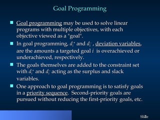
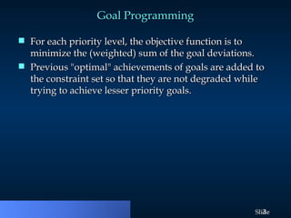
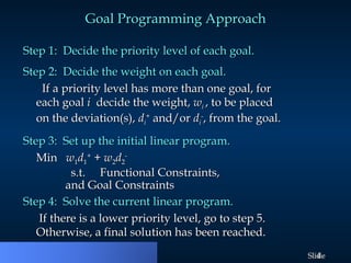
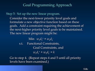
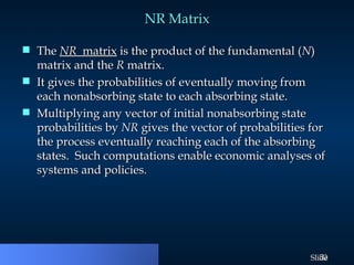
Goal programming is a mathematical method used to solve linear programs with multiple objectives, treating each objective as a goal. It utilizes deviation variables to measure goals' overachievement or underachievement, and prioritizes them in a sequential manner to minimize goal deviations. The approach includes formulating linear programs based on prioritized goals and ensuring higher priority goals are maintained while working towards lower priority objectives.


![54
© 2003 Thomson
© 2003 Thomson
/South-Western
/South-Western Slide
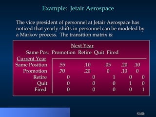
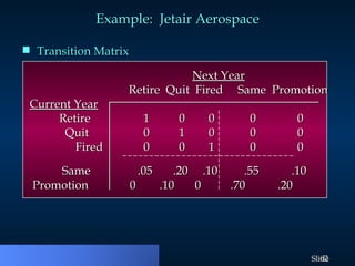
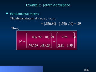
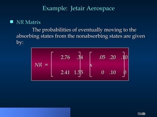
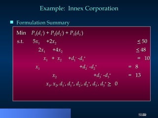
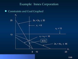
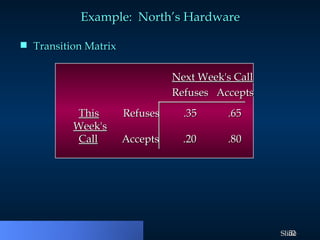
Example: North’s Hardware
Example: North’s Hardware
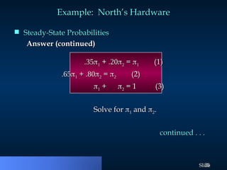
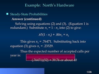
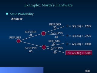
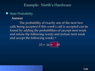
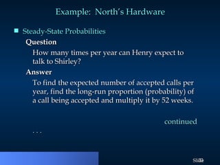
Steady-State Probabilities
Steady-State Probabilities
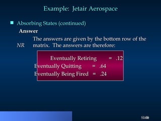
Answer
Answer (continued)
(continued)
Let
Let
1
1 = long run proportion of refused calls
= long run proportion of refused calls
2
2 = long run proportion of accepted calls
= long run proportion of accepted calls
Then,
Then,
.35 .65
.35 .65
[
[
] = [
] = [
]
]
.20 .80
.20 .80
continued . . .
continued . . .](https://image.slidesharecdn.com/goalprogramming-240930101424-41e6da91/85/introduction-of-the-Goal-Programming-ppt-54-320.jpg)