waves

1. Hydraulics 3 Waves: Random Waves and Statistics – 1 Dr David Apsley
3. RANDOM WAVES AND STATISTICS AUTUMN 2022
Real wave fields are not regular, but a combination of many components of different amplitude,
frequency and direction, which may be assumed to follow some statistical distribution. For
design, models must reflect the appropriate probability distributions of heights and spectral
distribution of frequencies (and, ideally, direction).
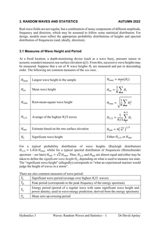
3.1 Measures of Wave Height and Period
At a fixed location, a depth-monitoring device (such as a wave buoy, pressure sensor or
acoustic sounder) measures sea-surface elevation η(𝑡). From this, successive wave heights may
be measured. Suppose that a set of 𝑁 wave heights 𝐻𝑖 are measured and put in descending
order. The following are common measures of the sea state.
𝐻max Largest wave height in the sample 𝐻max = max
𝑖
(𝐻𝑖)
𝐻av Mean wave height 𝐻av =
1
𝑁
∑ 𝐻𝑖
𝐻rms Root-mean-square wave height 𝐻rms = √
1
𝑁
∑ 𝐻𝑖
2
𝐻1 3
⁄ Average of the highest 𝑁/3 waves 𝐻1 3
⁄ =
1
𝑁/3
∑ 𝐻𝑖
𝑁/3
1
𝐻𝑚0 Estimate based on the rms surface elevation 𝐻𝑚0 = 4( 𝜂2
̅̅̅ )
1 2
⁄
𝐻𝑠 Significant wave height Either 𝐻1 3
⁄ or 𝐻𝑚0
For a typical probability distribution of wave heights (Rayleigh distribution)
𝐻1 3
⁄ = 1.416 𝐻rms, whilst for a typical spectral distribution of frequencies (Bretschneider
spectrum – see later) 𝐻𝑚0 = √2 𝐻rms. Thus, 𝐻1/3 and 𝐻𝑚0 are almost equal and either may be
taken to define the significant wave height 𝐻𝑠, depending on what is used to measure sea state.
The “significant wave height” (allegedly) corresponds to “what an experienced mariner would
judge the height of waves in a storm”.
There are also common measures of wave period:
𝑇𝑠 Significant wave period (average over highest 𝑁/3 waves)
𝑇𝑝 Peak period (corresponds to the peak frequency of the energy spectrum)
𝑇𝑒
Energy period (period of a regular wave with same significant wave height and
power density; used in wave-energy prediction; derived from the energy spectrum)
𝑇𝑧 Mean zero up-crossing period

2. Hydraulics 3 Waves: Random Waves and Statistics – 2 Dr David Apsley
3.2 Probability Distribution of Wave Heights
For a narrow-banded sea state (i.e. a small range of frequencies) deep-water waves have been
observed to follow a Rayleigh Distribution, for which the probability that wave heights exceed
𝐻 is given by
𝑃(height > 𝐻) = exp[−(𝐻/𝐻rms)2]
Thus,
cumulative distribution function: 𝐹(𝐻) = 𝑃(height < 𝐻) = 1 − e−(𝐻/𝐻rms)2
probability density function: 𝑓(𝐻) =
d𝐹
𝑑𝐻
= 2
𝐻
𝐻rms
2
e−(𝐻/𝐻rms)2
By definition of a probability density function, the probability that an individual wave height
lies between 𝐻1 and 𝐻2 is
𝑃(𝐻1 < 𝐻 < 𝐻2) = ∫ 𝑓(𝐻) d𝐻
𝐻2
𝐻1
= 𝐹(𝐻2) − 𝐹(𝐻1)
= e−(𝐻1/𝐻rms)2
− e−(𝐻2/𝐻rms)2
The only parameter of this distribution is the root-mean-square height, 𝐻rms. Exercise: verify
from probability theory, i.e.
𝐸(𝐻2) ≡ ∫ 𝐻2
𝑓(𝐻) d𝐻
∞
0
that E(𝐻2) = 𝐻rms
2
.
Other key wave statistics may be determined by the usual rules for probability distributions:
𝐻av ≡ 𝐸(𝐻) = ∫ 𝐻 𝑓(𝐻) d𝐻
∞
0
𝐻𝑝 = average of highest fraction 𝑝 of waves =
1
𝑝
∫ 𝐻 𝑓(𝐻) d𝐻
∞
𝐹−1(1−𝑝)

3. Hydraulics 3 Waves: Random Waves and Statistics – 3 Dr David Apsley
With this we find1
:
𝐻av =
√π
2
𝐻rms = 0.886 𝐻rms
𝐻1/3 = 1.416 𝐻rms
𝐻1 10
⁄ = 1.800 𝐻rms
𝐻1 100
⁄ = 2.359 𝐻rms
Example:
Near a pier, 400 consecutive wave heights are measured. Assume that the sea state is narrow-
banded.
(a) How many waves are expected to exceed 2𝐻rms?
(b) If the significant wave height is 2.5 m, what is 𝐻rms?
(c) Estimate the wave height exceeded by 80 waves.
(d) Estimate the number of waves with a height between 1.0 m and 3.0 m.
1
A certain amount of fiddly mathematics gives for the average of the highest fraction 𝑝:
𝐻𝑝
𝐻rms
= √ln(1/𝑝) +
√π
2𝑝
erfc(√ln(1/𝑝))
Here erfc() is the complementary error function, which most modern computer languages will
provide as a library function. Here it is in Python:
from math import sqrt, log, erfc, pi
def prob( p ):
x = sqrt( log( 1 / p ) )
return x + sqrt( pi ) / ( 2 * p ) * erfc( x )
p = float( input( "Enter p: " ) )
print( "H/Hrms = ", prob( p ) )

4. Hydraulics 3 Waves: Random Waves and Statistics – 4 Dr David Apsley
3.3 Wave Spectra
For regular waves of a single frequency, the wave energy (per unit surface area) is given by
𝐸 =
1
2
𝜌𝑔𝐴2
= 𝜌𝑔𝜂2(𝑡) =
1
8
𝜌𝑔𝐻2
i.e. the wave energy is proportional to the square of the amplitude 𝐴 (or height 𝐻) of the
harmonically-varying surface displacement 𝜂(𝑡).
Real wave fields contain many frequencies. The energy spectrum or power-spectral density
𝑆(𝑓) is such that the amount of energy (divided by ρ𝑔) in the small frequency interval d𝑓 is
𝑆(𝑓) d𝑓
or, equivalently, that the energy from waves between frequencies 𝑓1 and 𝑓2 is (𝜌𝑔 times)
∫ 𝑆(𝑓) d𝑓
𝑓2
𝑓1
(This is rather like a continuous probability distribution). Note that we can just as well work in
wave angular frequency 𝜔, where 𝜔 = 2π𝑓. In that case,
𝑆(𝜔) d𝜔
is the energy (divided by 𝜌𝑔) between wave angular frequencies 𝜔1 and 𝜔2.
3.3.1 Bretschneider Spectrum
Various model spectra are used in design. The Bretschneider spectrum is recommended for use
in open-ocean conditions:
𝑆(𝑓) =
5
16
𝐻𝑚0
2
𝑓
𝑝
4
𝑓5
exp (−
5
4
𝑓𝑝
4
𝑓4
)
where 𝐻𝑚0 is a measure of significant wave height 𝐻𝑠 based on the total energy (see below)
and 𝑓𝑝 is the peak frequency (= 1/𝑇𝑝, where 𝑇𝑝 is the peak period).

5. Hydraulics 3 Waves: Random Waves and Statistics – 5 Dr David Apsley
If we integrate over all frequencies we obtain total energy (strictly, energy divided by 𝜌𝑔):
𝐸
𝜌𝑔
≡ ∫ 𝑆(𝑓) d𝑓
∞
0
=
1
16
𝐻𝑚0
2
Hence
𝐻𝑚0 = 4√𝐸/𝜌𝑔 = 4√𝜂2(𝑡)
For a regular wave with height 𝐻rms (there is only one wave height, so it is the rms value):
𝐸
𝜌𝑔
=
1
8
𝐻rms
2
Thus, the complete spectrum with height parameter 𝐻𝑚0 will have the same energy density as
a regular wave with parameter 𝐻rms provided
𝐻𝑚0 = √2𝐻𝑟𝑚𝑠 = 1.414𝐻rms
But, for a Rayleigh distribution of wave heights, we have already seen that
𝐻𝑠 = 𝐻1/3 = 1.416𝐻rms
Hence, in practice, either 𝐻𝑚0 and 𝐻1/3 can be used synonymously for 𝐻𝑠.
3.3.2 Use of Spectral Data to Determine height and Period Parameters
From, e.g, wave-buoy data for 𝜂(𝑡), the power spectrum 𝑆(𝑓) can be determined by a discrete
Fourier transform of 𝜂2
. From this, as seen above, we can deduce immediately the peak period
𝑇𝑝 from the peak frequency in 𝑆(𝑓):
𝑇𝑝 =
1
𝑓𝑝
and the significant wave height
𝐻𝑠 = 𝐻𝑚0 = 4√𝑚0
where 𝑚0 is the zeroth moment: the area under the 𝑆(𝑓) curve. Other moments can be defined:
𝑚𝑛 = ∫ 𝑓𝑛
𝑆(𝑓) d𝑓
∞
0
and found from an experimentally-derived spectrum by numerical integration2
. A particularly
important one is 𝑚−1, since this can be used to determine the energy period 𝑇𝑒 (the period of
a regular wave with the same significant wave height and power density, which is widely used
in wavepower prediction):
𝑇𝑒 =
𝑚−1
𝑚0
and the zero up-crossing period 𝑇𝑧, which can be estimated from the wave spectrum by:
2
For the Bretschneider spectrum, some moderate mathematics produces 𝑚𝑛 =
1
16
𝐻𝑚0
2
𝑓𝑝
𝑛
(
5
4
)
𝑛
4
Γ(1 −
𝑛
4
) , where
Γ() is the gamma function (a generalisation of a factorial function).

6. Hydraulics 3 Waves: Random Waves and Statistics – 6 Dr David Apsley
𝑇𝑧 = √
𝑚0
𝑚2
For the Bretschneider spectrum these give
𝑇𝑒 = 0.857𝑇𝑝 (energy period)
𝑇𝑧 = 0.710𝑇𝑝 (zero up-crossing period)
3.3.3 The JONSWAP Spectrum
Another widely-used spectrum recommended for fetch-limited conditions (based on extensive
wave data from the North Sea) is the JONSWAP spectrum
𝑆(𝑓) = 𝐶𝐻𝑚0
2
𝑓𝑝
4
𝑓5
exp (−
5
4
𝑓
𝑝
4
𝑓4
) 𝛾𝑏
Here, the peak of the spectrum is enhanced (i.e. a greater proportion of the total energy is
clustered around the peak frequency) by the factor 𝛾𝑏
, where 𝛾 may be fitted to real
measurements, but is typically 3.3 and
𝑏 = exp {−
1
2
(
𝑓/𝑓
𝑝 − 1
𝜎
)
2
} , 𝜎 = {
0.07 𝑓 < 𝑓
𝑝
0.09 𝑓 > 𝑓
𝑝
C is the constant required to get the correct total energy (e.g.by numerical integration). A
JONSWAP spectrum is recommended for seas with more limited fetch.
For a JONSWAP spectrum (with 𝛾 = 3.3) numerical integration gives other design periods:
𝑇𝑒 = 0.903𝑇𝑝 (energy period)
𝑇𝑧 = 0.778𝑇𝑝 (zero up-crossing period)
3.3.4 Multi-Modal Spectra
Real sea states may contain waves from multiple sources – often waves of lower frequency
from a far-off storm (“swell”) and higher-frequency waves from a local storm (“wind”).
Complex statistical techniques can be used to extract the separate contributions from the
combined spectrum.
frequency f (Hz)
spectral
density
S
(m^2
s)
swell
wind

7. Hydraulics 3 Waves: Random Waves and Statistics – 7 Dr David Apsley
3.4 Constructing a Representative Wave Field From a Spectrum
For most spectra there is negligible energy associated with frequencies less than 0.5 𝑓
𝑝 or
greater than 3𝑓
𝑝, where 𝑓𝑝 is the peak frequency. If we break this or a larger frequency range
up into discrete intervals of length Δ𝑓, we can simulate a realistic spectrum (either in a
numerical simulation, or in a wave tank with programmable wave paddle) as a sum of
individual harmonic components:
𝜂(𝑡) = ∑ 𝑎𝑖cos (𝑘𝑖𝑥 − 𝜔𝑖𝑡 − 𝜙𝑖)
where 𝜔𝑖 and 𝑘𝑖 are the wavenumbers associated with frequency 𝑓𝑖, the 𝜙𝑖 are random phases,
and the correct amount of energy (𝐸𝑖) at this frequency occurs if we take
𝑆(𝑓𝑖)Δ𝑓 = 𝐸𝑖 =
1
2
𝑎𝑖
2
or
𝑎𝑖 = √2𝑆(𝑓𝑖) Δ𝑓
The wave tanks at the University of Manchester are equipped with programmable wave paddles
that can create such realistic random wave fields for a given spectrum.
Note that, as different wavenumbers travel with different speeds, this wave form is not
propagated unchanged (as it would be for a regular wave), but evolves with time.
If, instead of choosing random phases 𝜙𝑖 we choose them deliberately such that waves
travelling at different speeds arrive at the same point at the same time it is possible to generate
focused wave groups, with the focusing producing a very large-amplitude disturbance at a
single instant. These worst-case scenarios are used to simulate extreme-wave events.

8. Hydraulics 3 Waves: Random Waves and Statistics – 8 Dr David Apsley
Example.
An irregular wavefield at a deep-water location is characterised by peak period of 8.7 s and
significant wave height of 1.5 m.
(a) Provide a sketch of a Bretschneider spectrum, labelling both axes with variables and
units and indicating the frequencies corresponding to both the peak period and the
energy period.
Note: Calculations are not needed for this part.
(b) Determine the power density (in kW m–1
) of a regular wave component with frequency
0.125 Hz that represents the frequency range 0.12 to 0.13 Hz of the irregular wave field.
Example.
Wave measurements are obtained from a stationary sensor located in deep water. The measured surface
elevation of an irregular wave can be modelled as the sum of four regular wave components:
(a) In the context of modelling an irregular wave, explain the meaning of the following
terms:
(i) significant wave height;
(ii) significant wave period;
(iii) duration-limited.
(b) Obtain the total power conveyed by these deep-water wave components per metre width
of wave crest if conditions were measured:
(i) with zero current;
(ii) with an opposing current of 1.0 m s–1
.
Period (s) 6 7 8 9
Amplitude (m) 0.8 1.2 0.8 0.4

9. Hydraulics 3 Waves: Random Waves and Statistics – 9 Dr David Apsley
3.5 Prediction of Wave Climate
Models for wave spectra generally require one to specify a representative wave height (e.g. 𝐻𝑠)
and period (𝑇𝑠 or 𝑇𝑝).
Waves are generated by wind stress on the water surface, whilst gravity provides the restoring
force. Thus, wave height and period are expected to be functions of:
• wind speed 𝑈 (conventionally the wind speed at 10 m above the surface);
• fetch 𝐹 (the distance over which the wind blows);
• duration 𝑡 of the storm;
• gravity, 𝑔.
By dimensional analysis,
𝐻𝑠~𝑈, 𝐹, 𝑡, 𝑔
This gives 5 variables, 2 independent dimensions (length and time), and hence 3 dimensionless
Π groups:
𝑔𝐻𝑠
𝑈2
= function(
𝑔𝐹
𝑈2
,
𝑔𝑡
𝑈
)
Similarly
𝑔𝑇𝑝
𝑈
= function(
𝑔𝐹
𝑈2
,
𝑔𝑡
𝑈
)
Extensive wave data has led to empirical forms for these. Two of the commonest are SMB
(Sverdrup, Monk and Bretschneider) and JONSWAP (JOint North Sea WAve Project).
These correlations can be used to predict wave climate (usually to construct a wave spectrum)
from a weather forecast (forecasting), ongoing weather (nowcasting) and reconstructing wave
climate from measured wind records (hindcasting).
The following are standard correlations for deep-water waves.
3.5.1 JONSWAP (Hasselman et al., 1973)
If the wind has blown long enough for wave energy to propagate right across the fetch then the
wave parameters become functions only of the fetch 𝐹 and cease to be dependent on the storm
duration 𝑡. These are called fetch-limited waves and an empirical correlation is
𝑔𝐻𝑠
𝑈2
= 0.0016 (
𝑔𝐹
𝑈2
)
1 2
⁄
(up to maximum 0.2433)
𝑔𝑇𝑝
𝑈
= 0.286 (
𝑔𝐹
𝑈2
)
1 3
⁄
(up to maximum 8.134)
The (fairly rare) “maximum” conditions correspond to a “fully-developed sea” – one for which
energy dissipation equals energy input and wave conditions become independent of fetch.
The minimum duration for fetch-limited waves, 𝑡min is given, in non-dimensional form by

10. Hydraulics 3 Waves: Random Waves and Statistics – 10 Dr David Apsley
(
𝑔𝑡
𝑈
)
min
= 68.8 (
𝑔𝐹
𝑈2
)
2 3
⁄
(fully − developed sea: 7.15 × 104
)
If the storm duration 𝑡 < 𝑡min then the wave conditions are said to be duration-limited and the
non-dimensional fetch 𝑔𝐹/𝑈2
in the equations for 𝐻𝑠 and 𝑇𝑃 has to be replaced by an effective
fetch 𝐹eff determined by rearranging the last equation in terms of the actual duration t:
(
𝑔𝐹
𝑈2
)
eff
= (
1
68.8
𝑔𝑡
𝑈
)
3 2
⁄
Note:
(1) The period parameter predicted here is the peak period 𝑇𝑝, since this is what is required in
the Jonswap spectrum. If required, the significant wave period can be estimated by
𝑇𝑠 ≈ 0.945𝑇𝑝
(2) It is a considerable nuisance to have to keep writing the Π groups out in full. The JONSWAP
equations are conveniently written (ignoring the fully-developed limit) as
𝐻
̂𝑠 = 0.0016𝐹
̂1 2
⁄
𝑇
̂𝑝 = 0.286𝐹
̂1 3
⁄
𝑡̂min = 68.8𝐹
̂2 3
⁄
where
𝐹
̂ ≡
𝑔𝐹
𝑈2
, 𝑡̂ ≡
𝑔𝑡
𝑈
, 𝐻
̂𝑠 ≡
𝑔𝐻𝑠
𝑈2
, 𝑇
̂𝑝 ≡
𝑔𝑇𝑝
𝑈
distance travelled by wave energy greater than fetch F
F
distance travelled by wave energy less than fetch F
F
Feff
FETCH-LIMITED
DURATION-LIMITED

11. Hydraulics 3 Waves: Random Waves and Statistics – 11 Dr David Apsley
3.5.2 SMB (Bretschneider, 1970)
This alternative correlation has slightly(!) more complex formulae. Note that the representative
period here is 𝑇𝑠, the significant wave period, rather than 𝑇𝑝, the peak period. In non-
dimensional form:
𝐻
̂𝑠 = 0.283 tanh{0.0125𝐹
̂0.42
}
𝑇
̂𝑠 = 7.54 tanh{0.077𝐹
̂0.25
}
The minimum storm duration for fetch-limited waves is given by
𝑡̂min = 𝐾 exp {√[𝐴(ln 𝐹
̂)
2
− 𝐵 ln 𝐹
̂ + 𝐶] + 𝐷 ln 𝐹
̂}
where 𝐾 = 6.5882, 𝐴 = 0.0161, 𝐵 = 0.3692, 𝐶 = 2.2024, 𝐷 = 0.8798.
Prediction curves; solid: JONSWAP; dashed: SMB
Example.
(a) Wind has blown at a consistent 𝑈 = 20 m s−1
over a fetch 𝐹 = 100 km for 𝑡 = 6 hrs.
Determine 𝐻𝑠 and 𝑇𝑝 using the JONSWAP curves.
(b) If the wind blows steadily for another 4 hours what are 𝐻𝑠 and 𝑇𝑝?