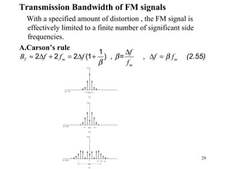
Download to read offline
![2
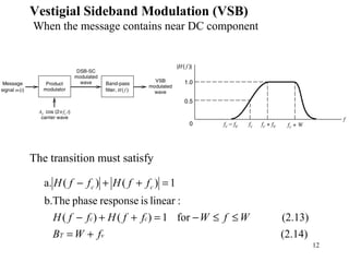
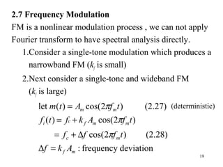
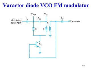
2.2 Consider a carrier
The output of the modulator
Where m(t) is the baseband signal , ka is the amplitude sensitivity.
(2.1))2cos()( tfAtc cc π=
[ ] (2.2))2cos()(1)( tftmkAts cac π+=
)(offreqencyhightesttheiswhere
(2.4).2
(2.3)tallfor,1)(.1
tmW
Wf
tmk
c
a
>>
<
X
1+kam(t) S(t
)
Accos(2πfct)](https://image.slidesharecdn.com/chapter2-171213110609/85/Chapter2-2-320.jpg)
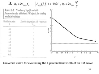
![3
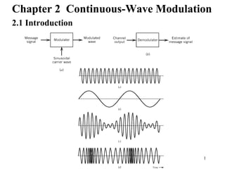
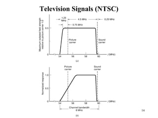
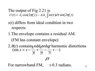
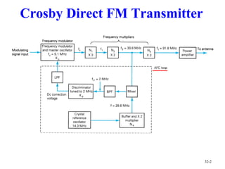
Recall
1.Negative frequency component of m(t) becomes visible.
2.fc-W < M(f) < fc lower sideband
fc < M(f) < fc+W upper sideband
3.Transmission bandwidth BT=2W
(2.2))2cos()()2cos()( tftmkAtfAts caccc ππ +=
[ ]
[ ]
[ ] [ ]
)(ofTransformFouriertheis)(where
(2.5))()(
2
)()(
2
)(
)()(
2
1
)2cos()(
)()(
2
1
)2cos(
tmfM
ffMffM
Ak
ffff
A
fs
ffMffMtftm
fffftf
cc
ca
cc
c
ccc
ccc
++−+++−=
++−⇔
++−⇔
δδ
π
δδπ](https://image.slidesharecdn.com/chapter2-171213110609/85/Chapter2-3-320.jpg)


![13
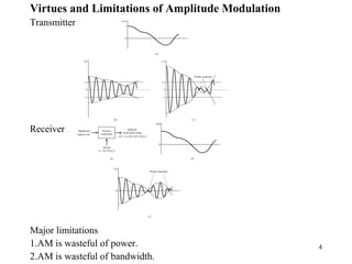
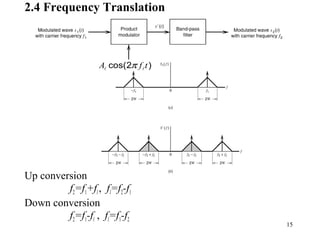
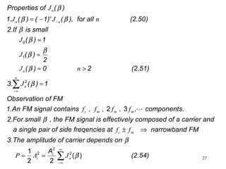
± corresponds to upper or lower sideband
(2.15))2sin()('
2
1
)2cos()(
2
1
)( tftmAtftmAts cccc ππ ±=
HQ(f)
m(t) m’(t)
[ ] (2.16)for)()()( WfWffHffHjfH ccQ ≤≤−+−−=](https://image.slidesharecdn.com/chapter2-171213110609/85/Chapter2-13-320.jpg)
![17
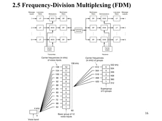
2.6 Angle Modulation
Basic Definitions:
Better discrimination against noise and interference
(expense of bandwidth).
The instantaneous frequency is
[ ] (2.19))(cos)( tAts ic θ=
constantiswhere
(2.22)2)(
is)(carrier,dunmodulateanFor
(2.21)
)(
2
1
2
)()(
lim
)(lim)(
0Δ
Δ
0Δ
c
cci
i
i
ii
t
t
t
i
tft
t
dt
td
t
ttt
tftf
φ
φπθ
θ
θ
π
π
θθ
+=
=
∆
−∆+
=
=
→
→](https://image.slidesharecdn.com/chapter2-171213110609/85/Chapter2-17-320.jpg)
![18
1. Phase modulation (PM)
2. Frequency Modulation (FM)
[ ] (2.23))(2cos
modulatortheofysensitivitphase:
)(2)(
tmktfAs(t)
k
tmktft
pcc
p
pci
+=
+=
π
πθ
(2.24)
ππ
ππ (2.26)
:frequency sensitivity of the modulator
compare (2.23) and (2.26)
0
0
( ) ( )
( ) 2 2 ( )
cos 2 2 ( )
i c f
t
i c f
t
c c f
f
p
f t f k m t
t f t k m d
s(t) A f t k m d
k
k m'
θ τ τ
τ τ
= +
= +
= +
⇒
∫
∫
π
0
2 ( )
t
f(t) k m dτ τ= ∫
(2.25)
generating FM signal generating PM signal](https://image.slidesharecdn.com/chapter2-171213110609/85/Chapter2-18-320.jpg)
![20
[ ]
radian.onenlarger thais,FMWideband
radian.oneansmaller this,FMNarrowband
(2.33))2sin(2cos)(
(2.32))2sin(2)(
(2.31)indexModulation
(2.30))2sin(2
)(2)((2.25),Recall
0
β
β
πβπ
πβθ
β
π
ττπθ
tftfAts
tftπft
f
f
tf
f
f
tπf
dft
mcc
mci
m
m
m
c
t
ii
+=
+=
∆
=
∆
+=
= ∫
(2.19) =>](https://image.slidesharecdn.com/chapter2-171213110609/85/Chapter2-20-320.jpg)
![21
Narrowband FM
[ ]
[ ] [ ]
[ ]
[ ]
(2.35))2sin()2sin()2cos()(
)2sin()2sin(sin
1)2sin(cos
small,isBecause
)34.2()2sin(sin)2sin()2sin(cos)2cos(
)2sin(2cos)(
tftfAtfAts
tftf
tf
tftfAtftfA
tftfAts
mcccc
mm
m
mccmcc
mcc
ππβπ
πβπβ
πβ
β
πβππβπ
πβπ
−≈
≈
≈
−=
+=](https://image.slidesharecdn.com/chapter2-171213110609/85/Chapter2-21-320.jpg)
![23
[ ] [ ]{ }
[ ]
[ ] [ ]{ } (2.37))(2cos)(2cos
2
1
)2(cos
)2cos()2(cos)2(cos
(2.2))2(cos)(1)(
)2cos()(,wavemodulatingsinusoidalAM withFor
(2.36))(2cos)(2cos
2
1
)2(cos
(2.35))2)sin(2(sin)2(cos)(
(2.35)Recall
AM
tfftffAtfA
tftfAktfA
tftmkAts
tftm
tfftffAtfA
tftfAtfAts
mcmcccc
mccacc
cac
m
mcmcccc
mcccc
−−++=
+=
+=
=
−−++≈
−≈
ππµπ
πππ
π
π
ππβπ
ππβπ
Narrow band FM
AM](https://image.slidesharecdn.com/chapter2-171213110609/85/Chapter2-23-320.jpg)
![24
Wideband FM (large B)
[ ]
[ ]
[ ]
[ ]
(2.40))2exp()(~
)]2sin(exp[)(~
bydefinedenvelopecomplextheis)(~
andpartrealthedenotesRewhere
(2.38)))(2exp()(~Re
))2sin(2exp(Re)(
sincosexp
(2.33))2sin(2cos)(
∑
∞
−∞=
=
=
=
+=
+=
+=
n
mn
mc
c
mcc
mcc
tnfjcts
tfjAts
ts
tfjts
tfjtfjAts
xjx(jx)
tftfAts
π
πβ
π
πβπ
πβπ
(2.39)
Complex Fourier Transform](https://image.slidesharecdn.com/chapter2-171213110609/85/Chapter2-24-320.jpg)
![25
[ ]
[ ]
(2.41)
Let (2.42)
1
2
1
2
1
2
1
2
( )exp( 2 )
exp sin(2 ) 2 )
2
exp ( sin )
2
m
m
m
m
f
n m mf
f
m c m mf
m
c
n
c f s t j nf t dt
f A j f t j nf t dt
x f t
A
c j x nx dx
π
β π π
π
β
π
−
−
= −
= −
=
= −
∫
∫
%
[ ]
2
(2.43)
Define the th order Bessel function of the first kind as
A3, x
(2.44)
2
2 2
2
( ) 0)
1
( ) exp ( sin )
2
( )
( ) ( )
n
n c n
c n
n
n
d y dy
x x n y
dx dx
J j x nx dx
c A J
s t A J
π
π
π
π
β β
π
β
β
−
−
=−
+ + − =
= −
=
=
∫
∫
% (2.45)exp( 2 )mj nf tπ
∞
∞
∑](https://image.slidesharecdn.com/chapter2-171213110609/85/Chapter2-25-320.jpg)
![26
[ ]
[ ]
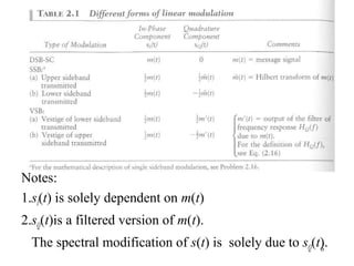
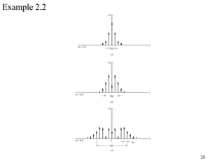
[ ] (2.49))()()(
2
)(
is)(ofransformFourier tThe
(2.48))(2cos)(
(2.47))(2exp)(Re)(
mcmcn
c
mcnc
mcnc
nfffnfffJ
A
fS
ts
tnffJA
tnffjJAts
+++−−=
+=
+=
∑
∑
∑
∞
∞−
∞
∞−
∞
∞−
δδβ
πβ
πβ
Figure 2.23 Plots of Bessel functions of the first kind for varying](https://image.slidesharecdn.com/chapter2-171213110609/85/Chapter2-26-320.jpg)

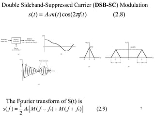
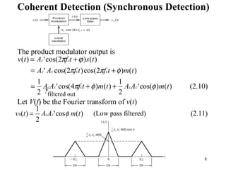
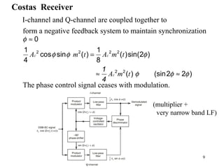
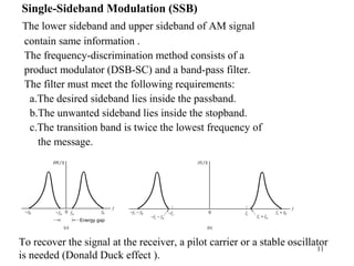
This document summarizes continuous-wave modulation techniques. It discusses amplitude modulation (AM), including the transmitter and receiver, and limitations of AM. It also covers linear modulation schemes like double sideband-suppressed carrier, single sideband, and vestigial sideband modulation. Frequency modulation techniques are analyzed, including narrowband and wideband FM. Bessel functions are used to describe the spectrum of wideband FM signals. Carson's rule and universal curves are presented for calculating the transmission bandwidth of FM signals.


![Multiband Transceivers - [Chapter 1]](https://cdn.slidesharecdn.com/ss_thumbnails/ch1-150613070932-lva1-app6891-thumbnail.jpg?width=640&height=640&fit=bounds)