Communication system unit 1 ppt about types of modulation and its derivatives and its power calculation.

1. UNIT-I
Amplitude Modulation System
1

2. Introduction to communications
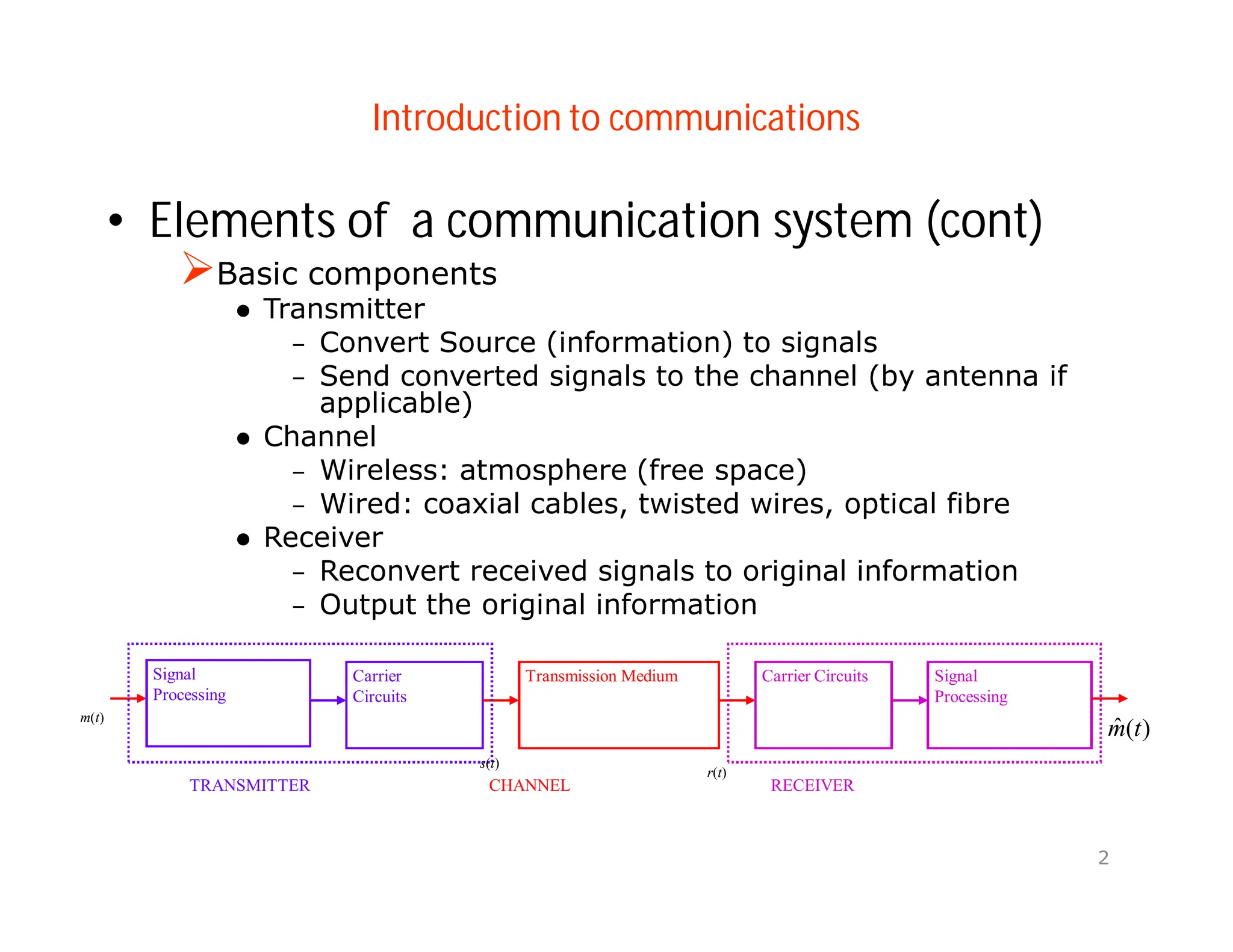
• Elements of a communication system (cont)
2
Basic components
 Transmitter
– Convert Source (information) to signals
– Send converted signals to the channel (by antenna if
applicable)
 Channel
– Wireless: atmosphere (free space)
– Wired: coaxial cables, twisted wires, optical fibre
 Receiver
– Reconvert received signals to original information
– Output the original information
m(t)
Signal
Processing
Carrier
Circuits
Transmission Medium Carrier Circuits Signal
Processing
TRANSMITTER RECEIVER
s(t)
r(t)
)
(
ˆ t
m
CHANNEL

3. Introduction to communications
• Elements of a communication system (cont)
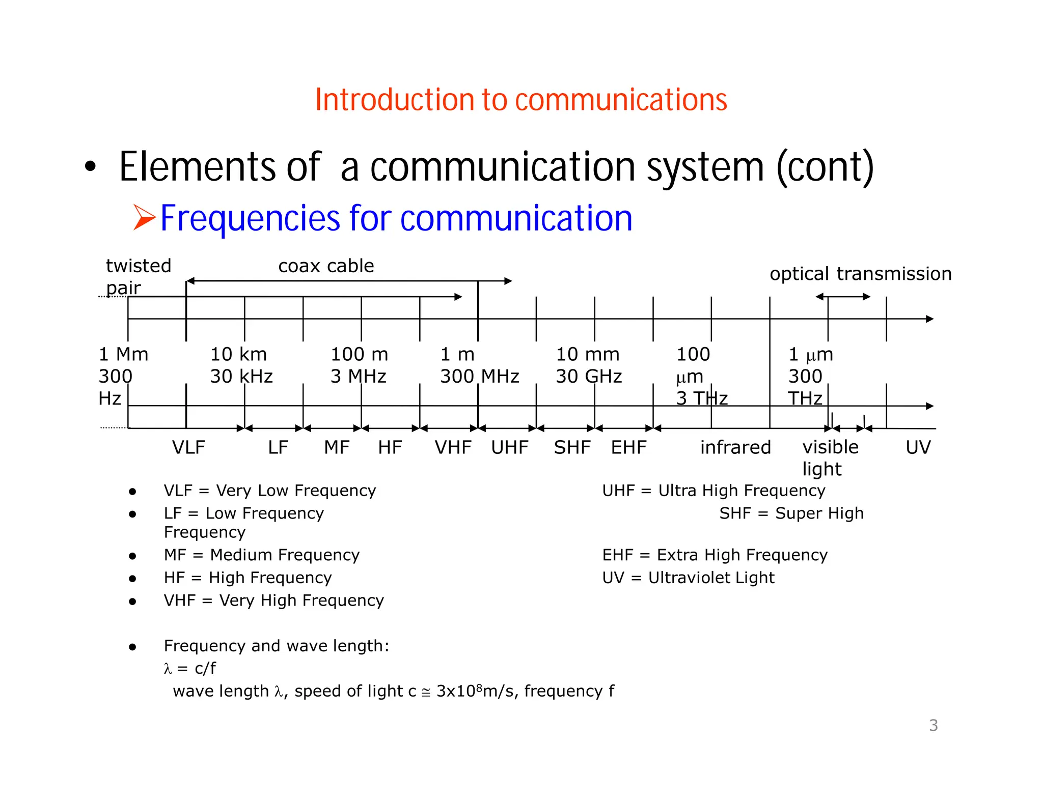
Frequencies for communication
3
1 Mm
300
Hz
10 km
30 kHz
100 m
3 MHz
1 m
300 MHz
10 mm
30 GHz
100
m
3 THz
1 m
300
THz
visible
light
VLF LF MF HF VHF UHF SHF EHF infrared UV
optical transmission
coax cable
twisted
pair
 VLF = Very Low Frequency UHF = Ultra High Frequency
 LF = Low Frequency SHF = Super High
Frequency
 MF = Medium Frequency EHF = Extra High Frequency
 HF = High Frequency UV = Ultraviolet Light
 VHF = Very High Frequency
 Frequency and wave length:
 = c/f
wave length , speed of light c  3x108m/s, frequency f

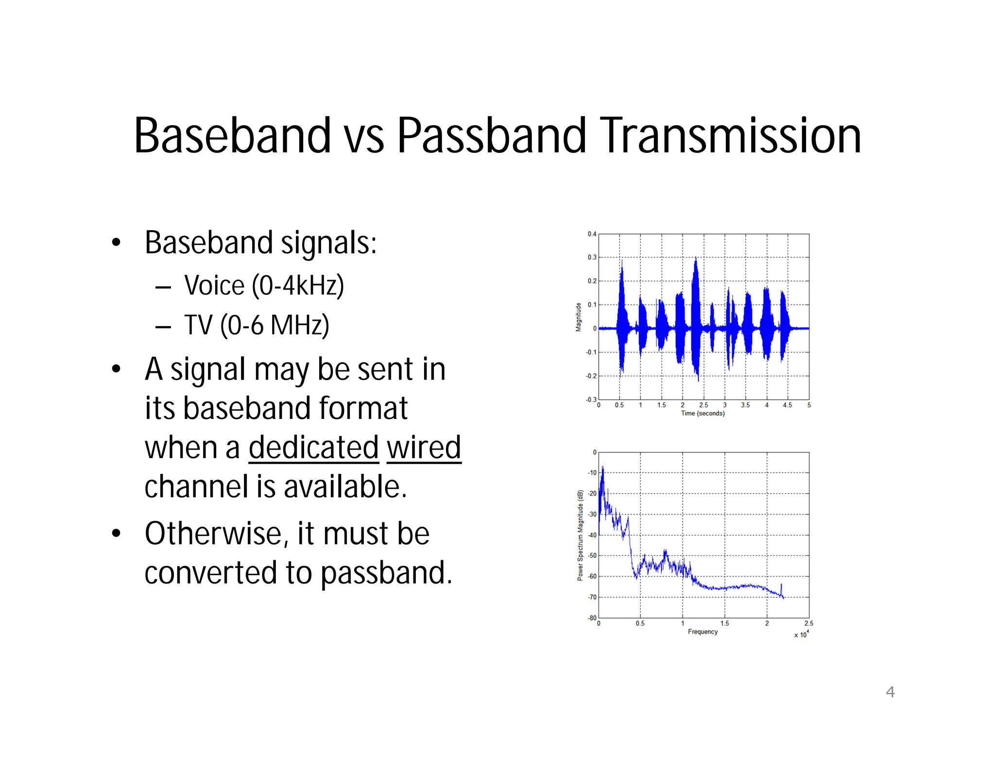
4. Baseband vs Passband Transmission
• Baseband signals:
– Voice (0-4kHz)
– TV (0-6 MHz)
• A signal may be sent in
its baseband format
when a dedicated wired
channel is available.
• Otherwise, it must be
converted to passband.
4

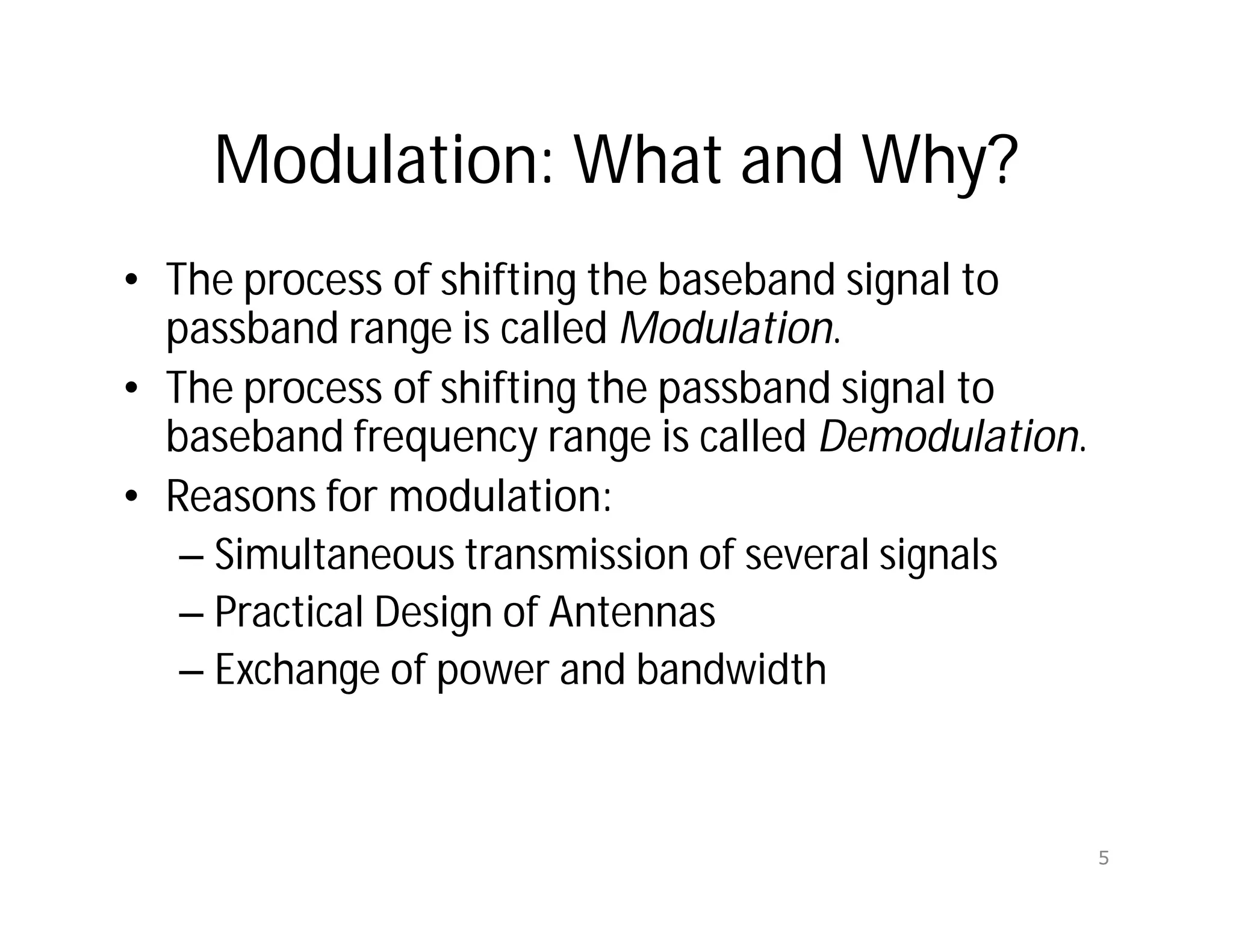
5. Modulation: What and Why?
• The process of shifting the baseband signal to
passband range is called Modulation.
• The process of shifting the passband signal to
baseband frequency range is called Demodulation.
• Reasons for modulation:
– Simultaneous transmission of several signals
– Practical Design of Antennas
– Exchange of power and bandwidth
5

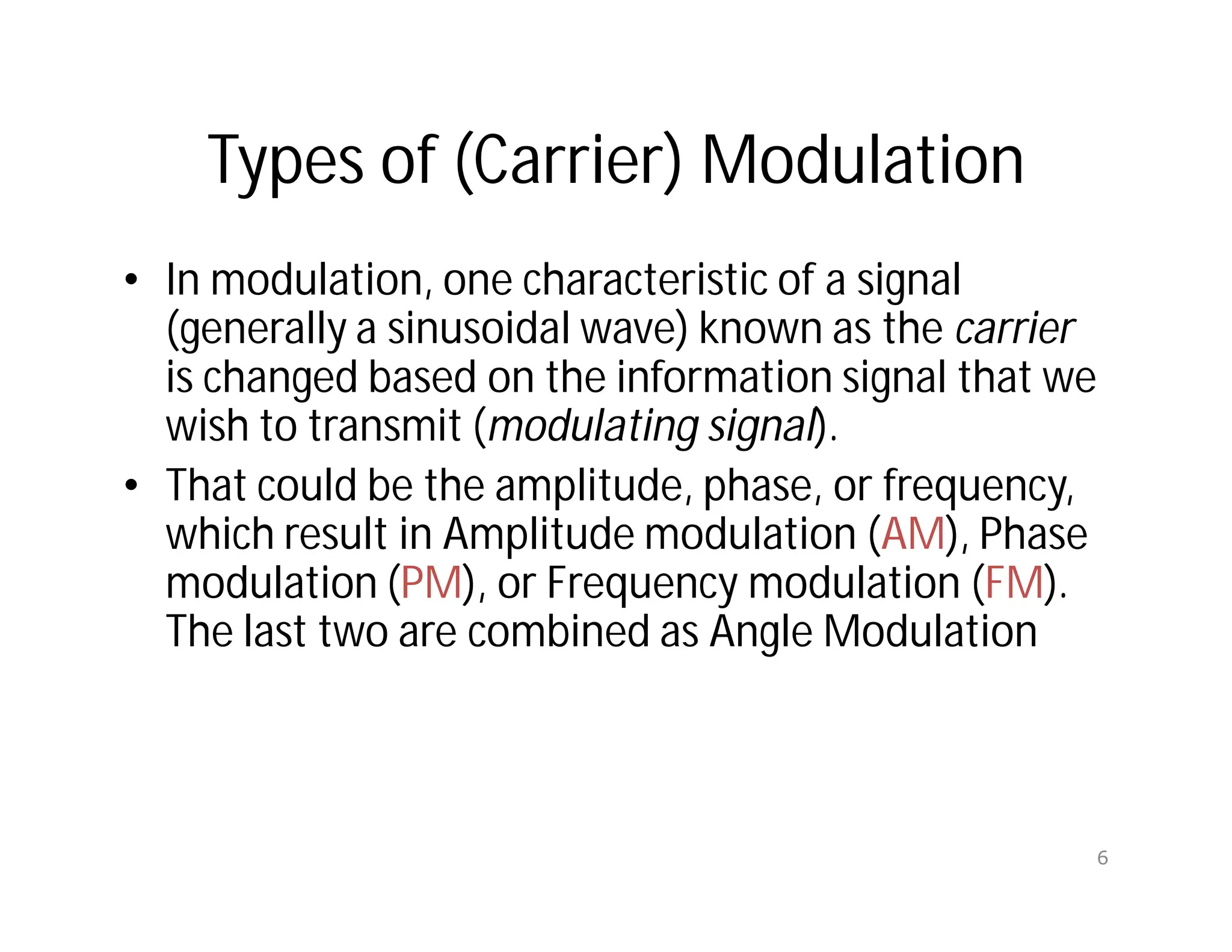
6. Types of (Carrier) Modulation
• In modulation, one characteristic of a signal
(generally a sinusoidal wave) known as the carrier
is changed based on the information signal that we
wish to transmit (modulating signal).
• That could be the amplitude, phase, or frequency,
which result in Amplitude modulation (AM), Phase
modulation (PM), or Frequency modulation (FM).
The last two are combined as Angle Modulation
6

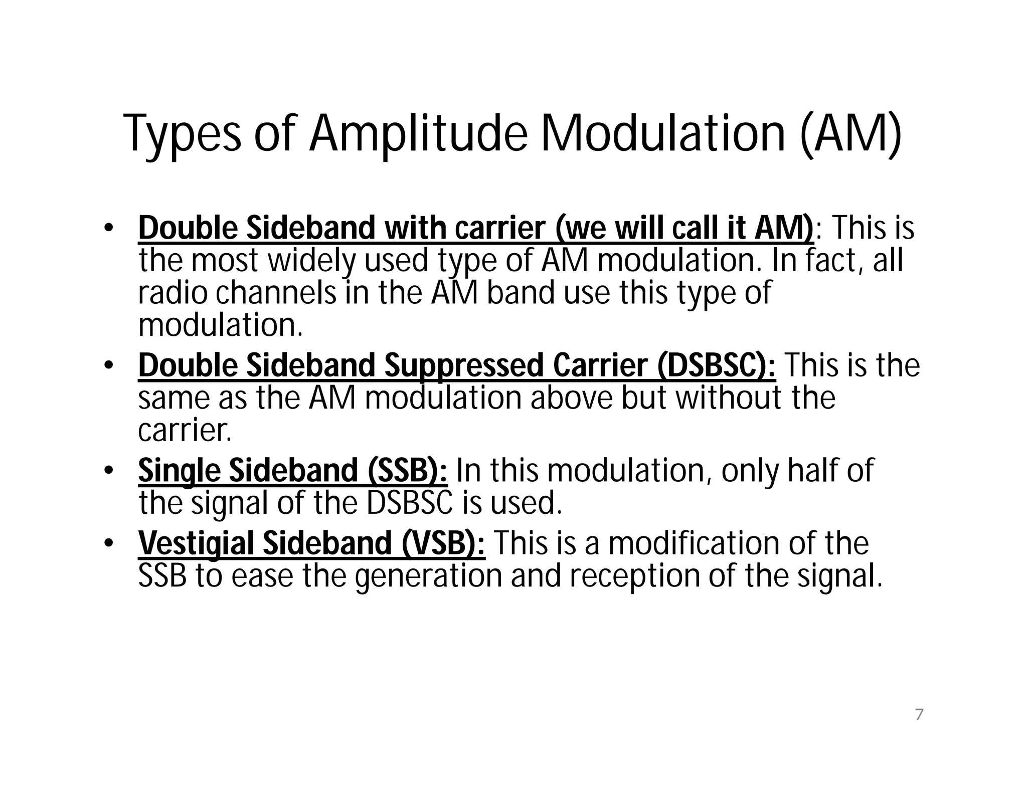
7. Types of Amplitude Modulation (AM)
• Double Sideband with carrier (we will call it AM): This is
the most widely used type of AM modulation. In fact, all
radio channels in the AM band use this type of
modulation.
• Double Sideband Suppressed Carrier (DSBSC): This is the
same as the AM modulation above but without the
carrier.
• Single Sideband (SSB): In this modulation, only half of
the signal of the DSBSC is used.
• Vestigial Sideband (VSB): This is a modification of the
SSB to ease the generation and reception of the signal.
7

8. Definition of AM
• Shift m(t) by some DC value “A”
such that A+m(t) ≥ 0. Or A ≥ mpeak
• Called DSBWC. Here will refer to it
as Full AM, or simply AM
• Modulation index m = mp /A.
• 0 ≤ m ≤ 1
)
cos(
)
(
)
cos(
)
cos(
)]
(
[
)
(
t
t
m
t
A
t
t
m
A
t
g
C
C
C
AM







8

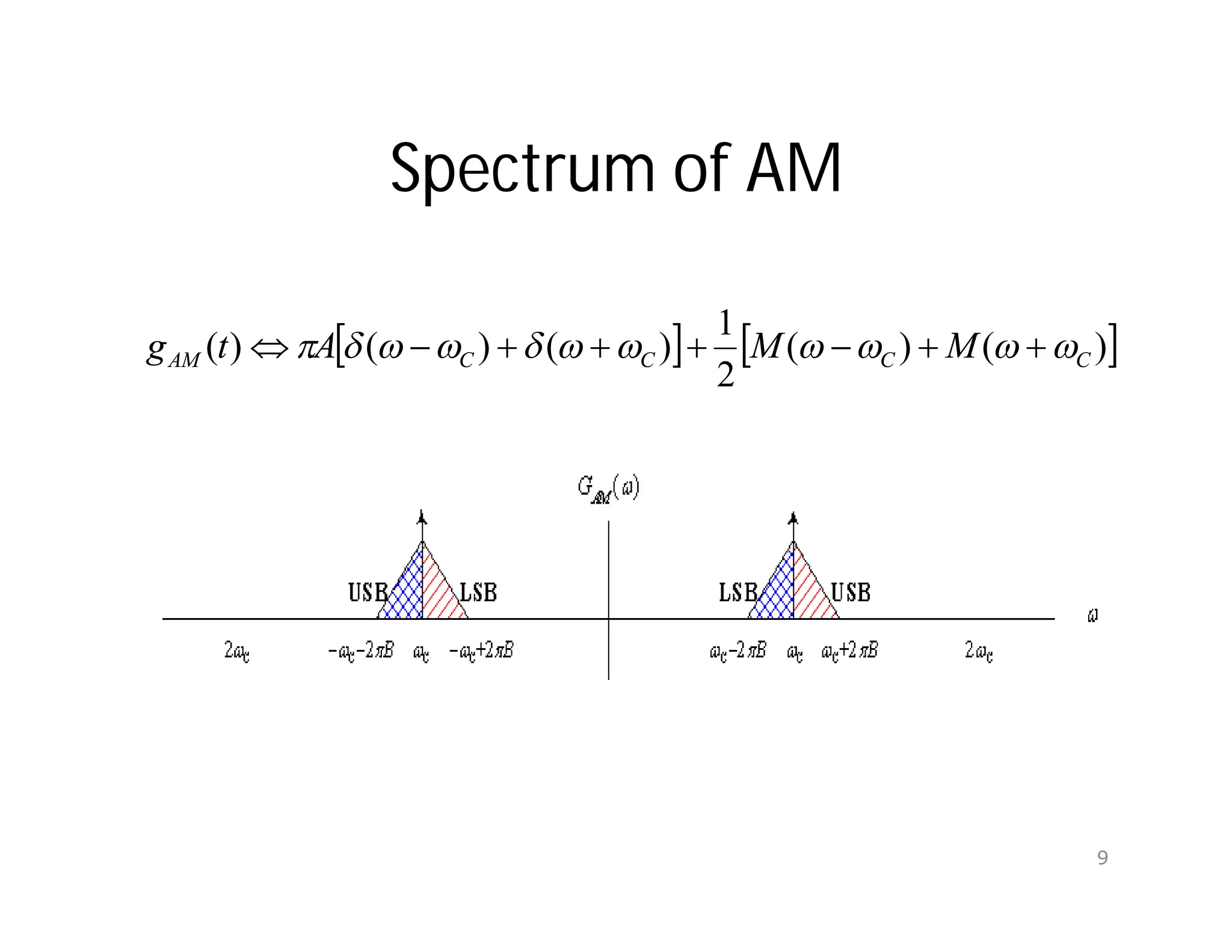
9. Spectrum of AM
   
)
(
)
(
2
1
)
(
)
(
)
( C
C
C
C
AM M
M
A
t
g 









 







9

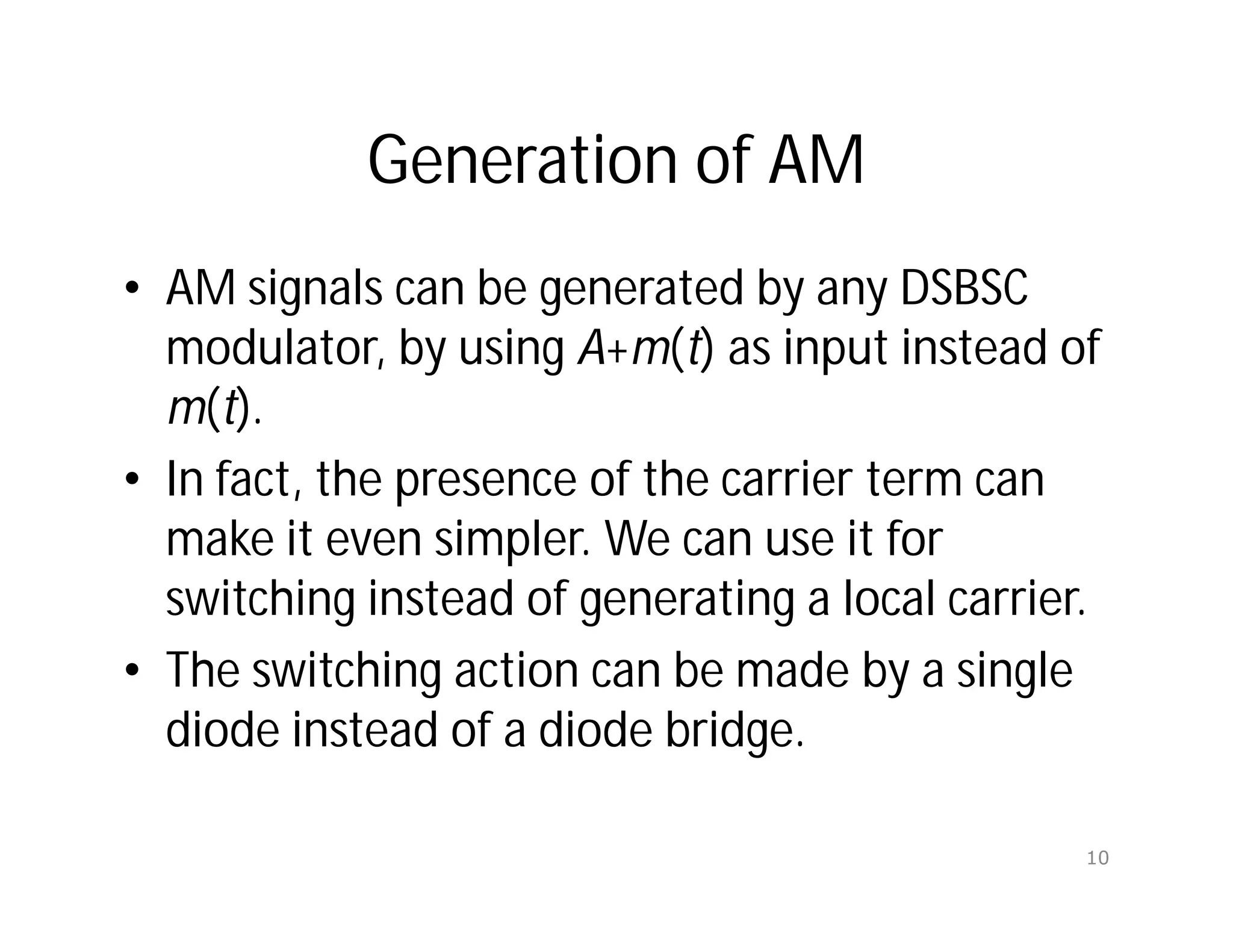
10. Generation of AM
• AM signals can be generated by any DSBSC
modulator, by using A+m(t) as input instead of
m(t).
• In fact, the presence of the carrier term can
make it even simpler. We can use it for
switching instead of generating a local carrier.
• The switching action can be made by a single
diode instead of a diode bridge.
10

11. AM Generator
• A >> m(t)
(to ensure switching
at every period).
• vR=[cosct+m(t)][1/2 + 2/p(cosct-1/3cos3ct + …)]
=(1/2)cosct+(2/p)m(t) cosct + other terms (suppressed by BPF)
• vo(t) = (1/2)cosct+(2/p)m(t) cosct
A
11

12. AM Modulation Process (Frequency)
12

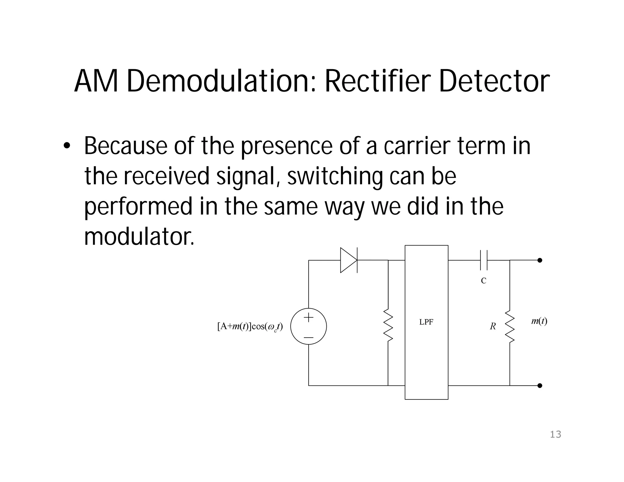
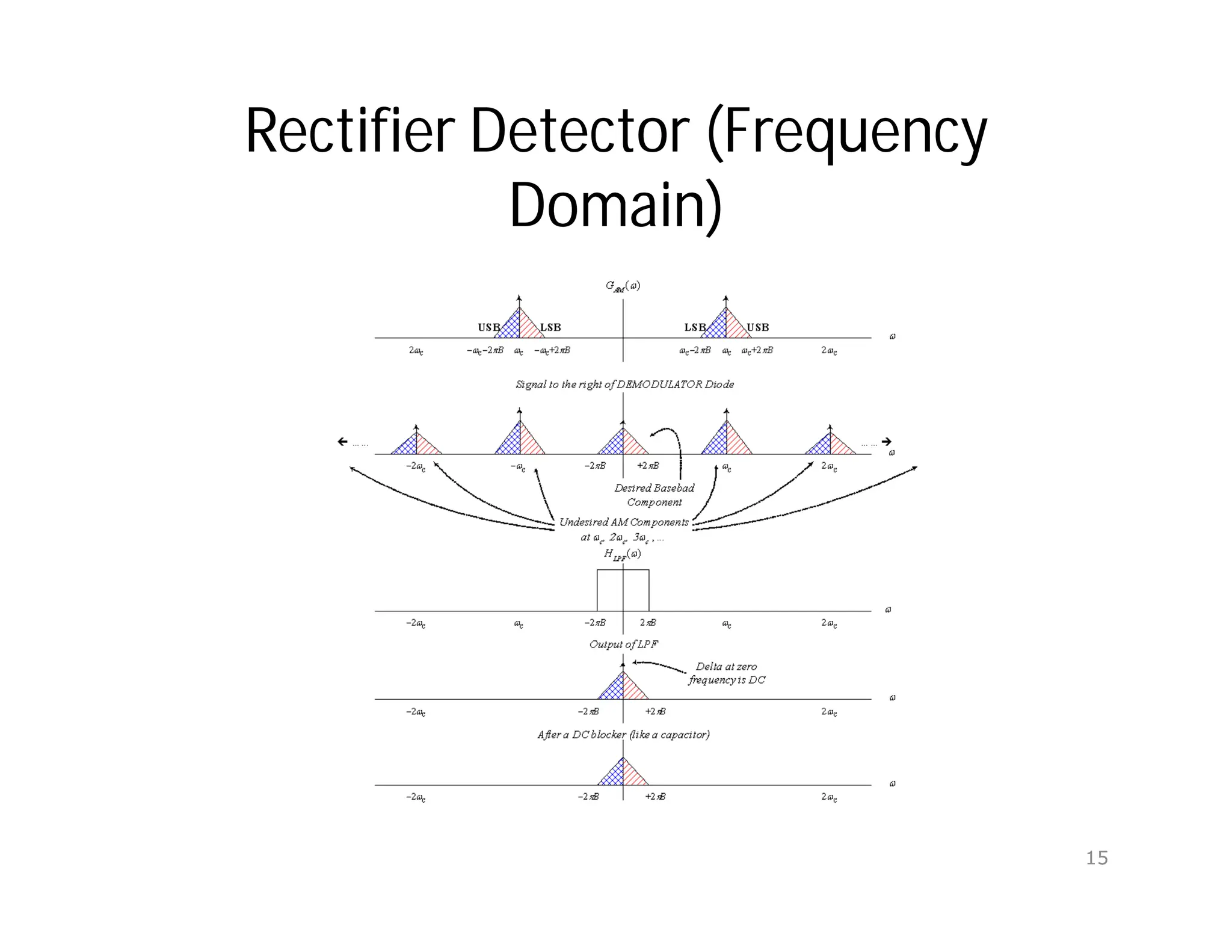
13. AM Demodulation: Rectifier Detector
• Because of the presence of a carrier term in
the received signal, switching can be
performed in the same way we did in the
modulator.
13

14. Rectifier Detector: Time Domain
14

15. Rectifier Detector (Frequency
Domain)
15

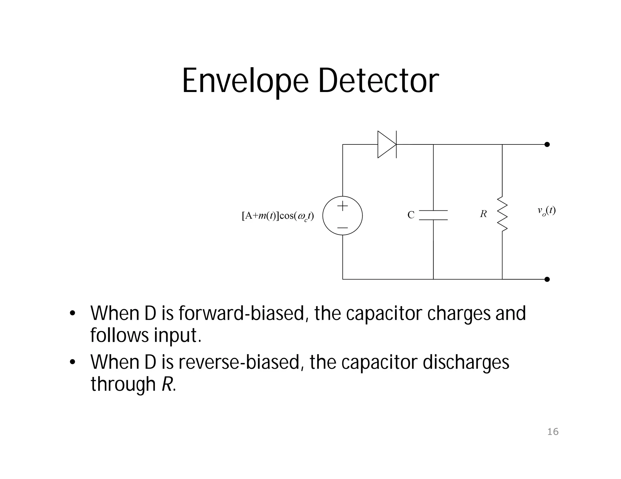
16. Envelope Detector
• When D is forward-biased, the capacitor charges and
follows input.
• When D is reverse-biased, the capacitor discharges
through R.
16

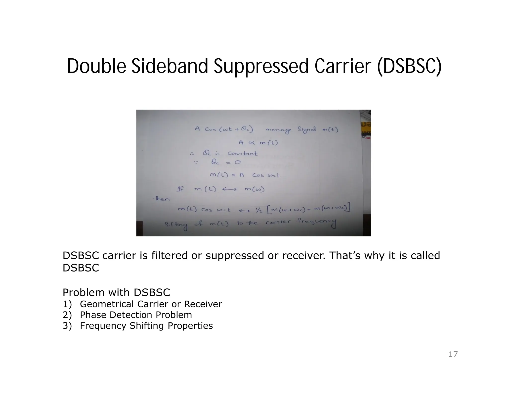
17. Double Sideband Suppressed Carrier (DSBSC)
DSBSC carrier is filtered or suppressed or receiver. That’s why it is called
DSBSC
Problem with DSBSC
1) Geometrical Carrier or Receiver
2) Phase Detection Problem
3) Frequency Shifting Properties
17

18. Time and Frequency Representation of DSBSC
Modulation Process
18

19. DSBSC Demodulation
Double Sideband Suppressed Carrier (DSBSC)
For a broadcast system it is more economical to have one
experience high power transmitter and expensive receiver, for such
application a large carrier signal is transmitted along with the
suppressed carrier modulated signal m(t) Cos (wct), thus no need
to generate a local carrier. This is called AM in which the
transmitted signal is.
Cos wct [ A + m(t) ]
19

20. Time and Frequency Representation of DSBSC
Demodulation Process
20

21. Modulator Circuits
• Basically we are after multiplying a signal with
a carrier.
• There are three realizations of this operation:
– Multiplier Circuits
– Non-Linear Circuits
– Switching Circuits
21

22. Non-Linear Devices (NLD)
• A NLD is a device whose input-output relation is non-
linear. One such example is the diode (iD=evD/vT).
• The output of a NLD can be expressed as a power series
of the input, that is
y(t) = ax(t) + bx2(t) + cx3(t) + …
• When x(t) << 1, the higher powers can be neglected, and
the output can be approximated by the first two terms.
• When the input x(t) is the sum of two signal, m(t)+c(t),
x2(t) will have the product term m(t)c(t)
22

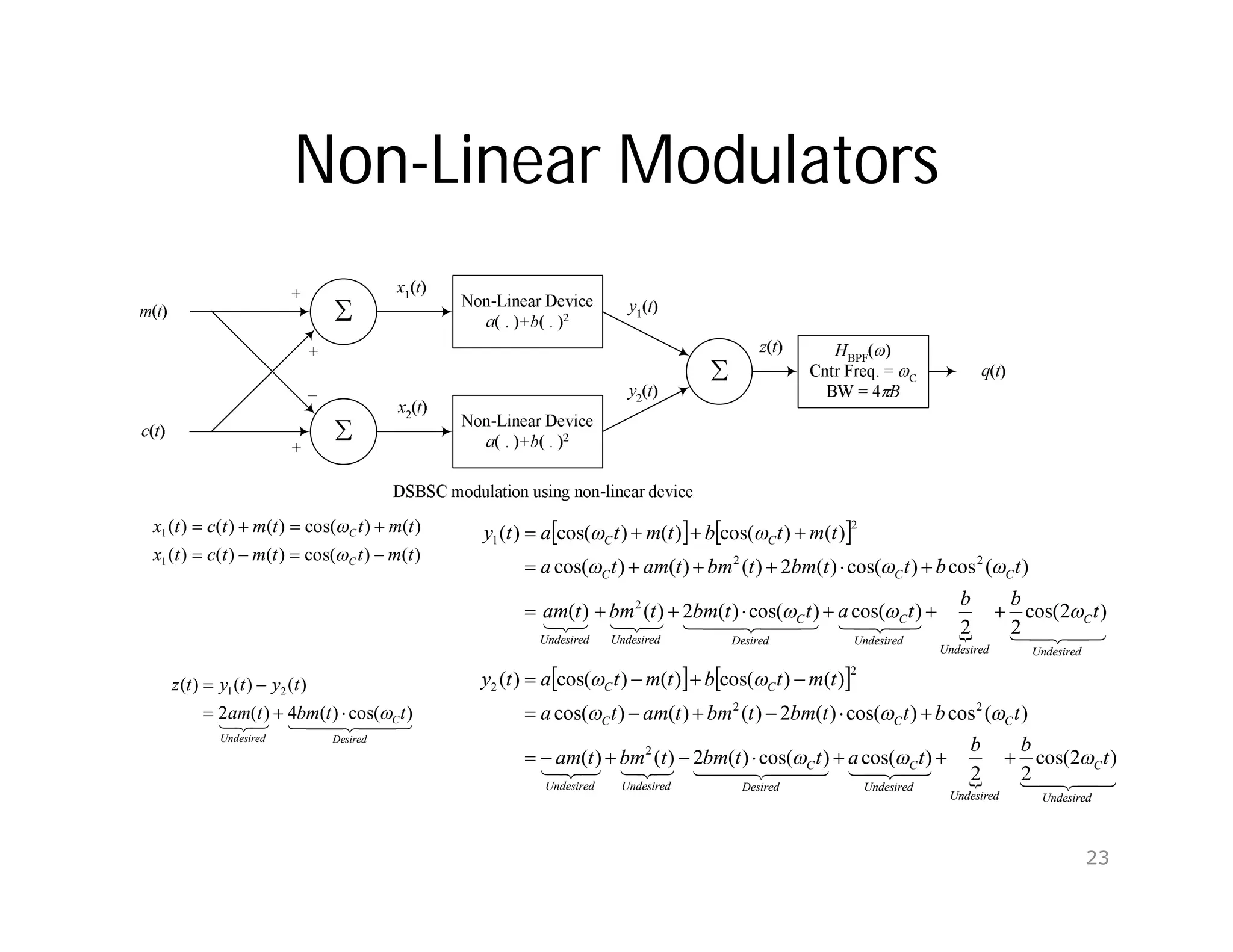
23. Non-Linear Modulators
   

   
 








 

 
















 

 







Undesired
C
Undesired
Undesired
C
Desired
C
Undesired
Undesired
C
C
C
C
C
Undesired
C
Undesired
Undesired
C
Desired
C
Undesired
Undesired
C
C
C
C
C
t
b
b
t
a
t
t
bm
t
bm
t
am
t
b
t
t
bm
t
bm
t
am
t
a
t
m
t
b
t
m
t
a
t
y
t
b
b
t
a
t
t
bm
t
bm
t
am
t
b
t
t
bm
t
bm
t
am
t
a
t
m
t
b
t
m
t
a
t
y
)
2
cos(
2
2
)
cos(
)
cos(
)
(
2
)
(
)
(
)
(
cos
)
cos(
)
(
2
)
(
)
(
)
cos(
)
(
)
cos(
)
(
)
cos(
)
(
)
2
cos(
2
2
)
cos(
)
cos(
)
(
2
)
(
)
(
)
(
cos
)
cos(
)
(
2
)
(
)
(
)
cos(
)
(
)
cos(
)
(
)
cos(
)
(
2
2
2
2
2
2
2
2
2
1



















































)
(
)
cos(
)
(
)
(
)
(
)
(
)
cos(
)
(
)
(
)
(
1
1
t
m
t
t
m
t
c
t
x
t
m
t
t
m
t
c
t
x
C
C











 

 




Desired
C
Undesired
t
t
bm
t
am
t
y
t
y
t
z
)
cos(
)
(
4
)
(
2
)
(
)
(
)
( 2
1






23

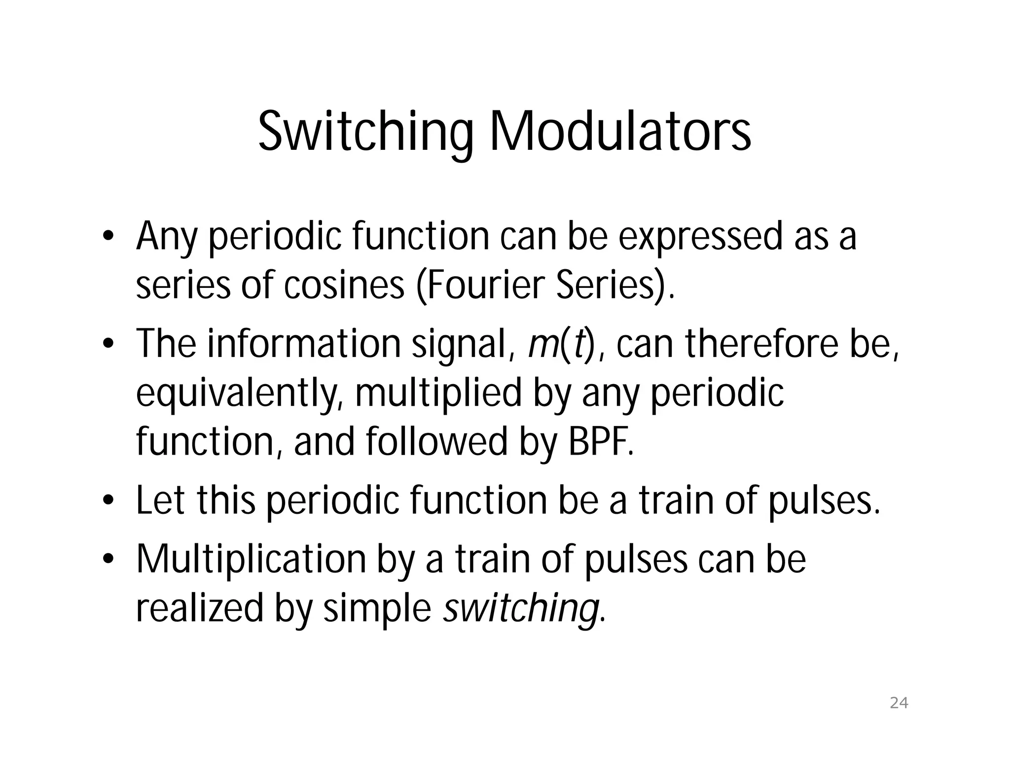
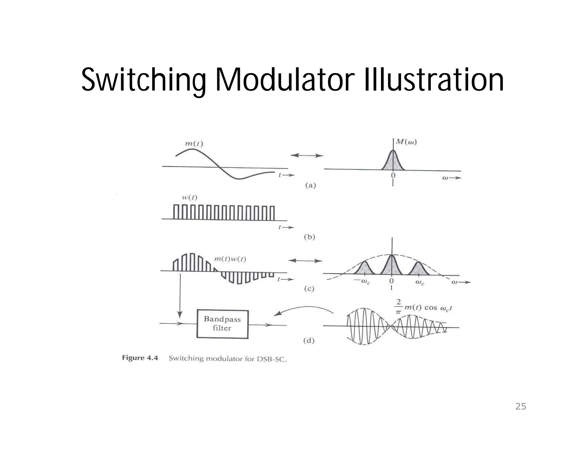
24. Switching Modulators
• Any periodic function can be expressed as a
series of cosines (Fourier Series).
• The information signal, m(t), can therefore be,
equivalently, multiplied by any periodic
function, and followed by BPF.
• Let this periodic function be a train of pulses.
• Multiplication by a train of pulses can be
realized by simple switching.
24

25. Switching Modulator Illustration
25

26. Switching Modulator: Diode Bridge
26

27. Switching Modulator: Ring
27

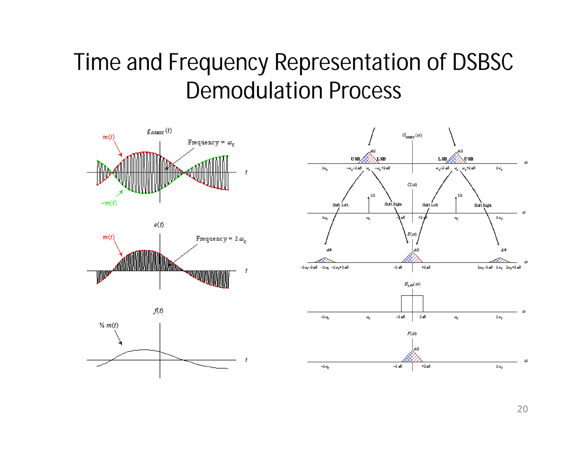
28. Demodulation of DSBSC
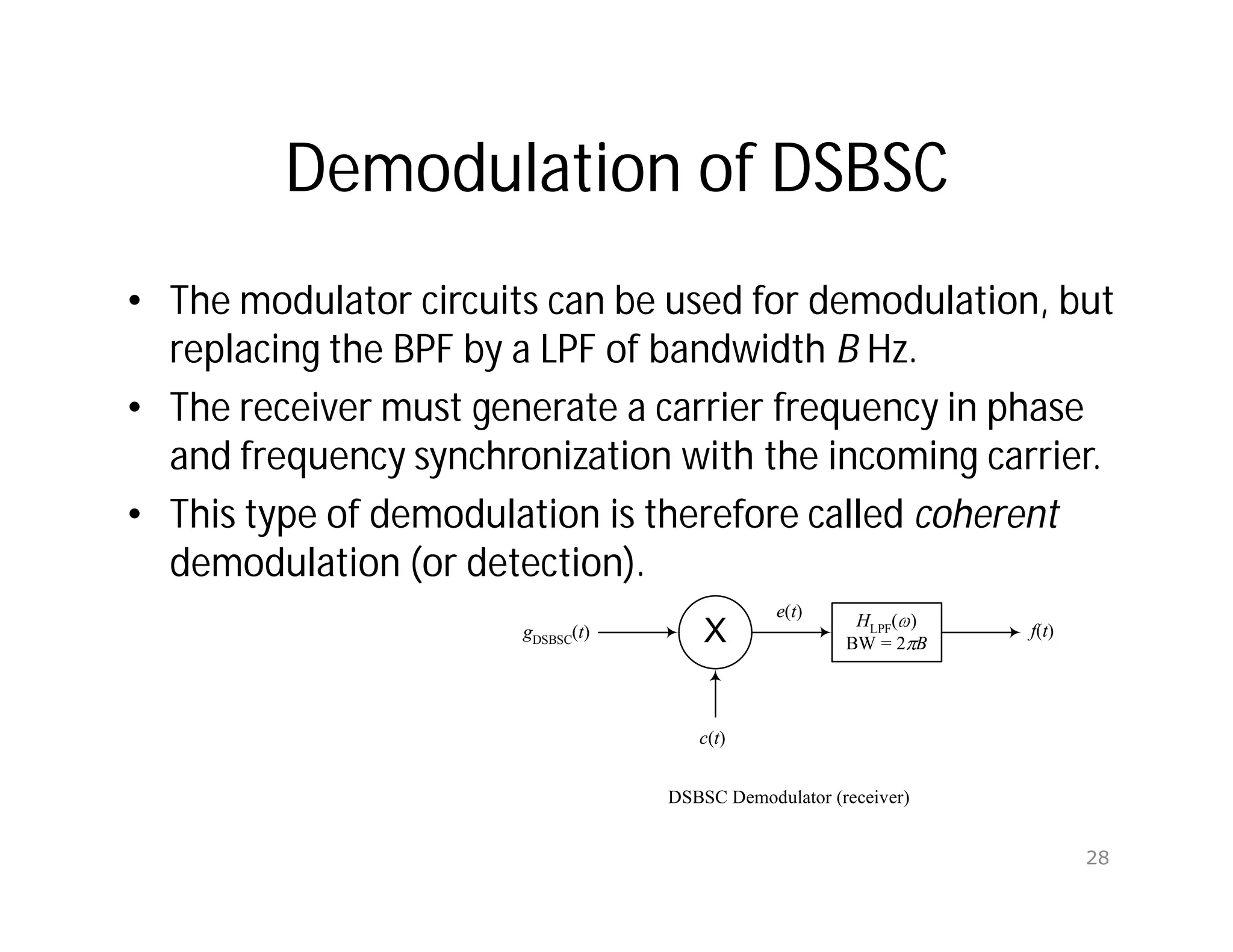
• The modulator circuits can be used for demodulation, but
replacing the BPF by a LPF of bandwidth B Hz.
• The receiver must generate a carrier frequency in phase
and frequency synchronization with the incoming carrier.
• This type of demodulation is therefore called coherent
demodulation (or detection).
X
c(t)
gDSBSC
(t)
e(t)
HLPF( )
BW = 2 B
f(t)
DSBSC Demodulator (receiver)
28

29. From DSBSC to DSBWC (AM)
• Carrier recovery circuits, which are required
for the operation of coherent demodulation,
are sophisticated and could be quite costly.
• If we can let m(t) be the envelope of the
modulated signal, then a much simpler circuit,
the envelope detector, can be used for
demodulation (non-coherent demodulation).
• How can we make m(t) be the envelope of the
modulated signal?
29

30. Single-Side Band (SSB) Modulation
• DSBSC (as well as AM) occupies double the bandwidth
of the baseband signal, although the two sides carry
the same information.
• Why not send only one side, the upper or the lower?
• Modulation: similar to DSBSC. Only change the settings
of the BPF (center frequency, bandwidth).
• Demodulation: similar to DSBSC (coherent)
30

31. SSB Representation
How would we represent
the SSB signal in the time
domain?
gUSB(t) = ?
gLSB(t) = ?
31

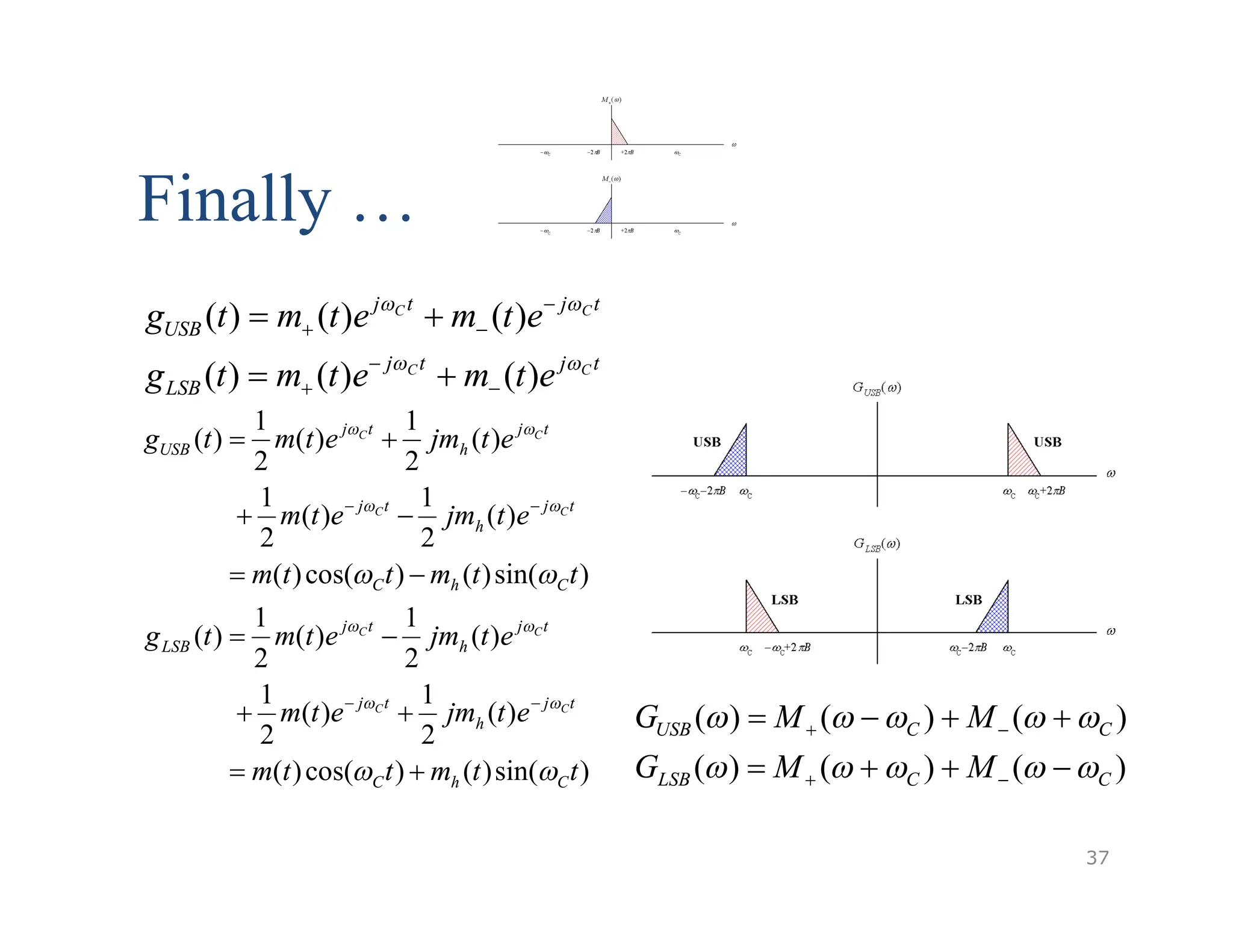
32. Time-Domain Representation of SSB (1/2)
M() = M+() + M-()
Let m+(t)↔M+() and m-(t)↔M-
()
Then: m(t) = m+(t) + m-(t) [linearity]
Because M+(), M-() are not even
 m+(t), m-(t) are complex.
Since their sum is real they must be
conjugates.
m+(t) = ½ [m(t) + j mh(t)]
m-(t) = ½ [m(t) - j mh(t)]
What is mh(t) ?
32

33. Time-Domain Representation of SSB (2/2)
M() = M+() + M-()
M+() = M()u(); M-() = M()u(-)
sgn()=2u() -1  u()= ½ + ½ sgn(); u(-) = ½ -½ sgn()
M+() = ½[ M() + M()sgn()]
M-() = ½ [M() - M()sgn()]
Comparing to:
m+(t) = ½ [m(t) + j mh(t)] ↔ ½ [M() + j Mh()]
m-(t) = ½ [m(t) - j mh(t)] ↔ ½ [M() - j Mh()]
We find
Mh() = - j M()∙sgn() where mh(t)↔Mh()
33

34. Hilbert Transform
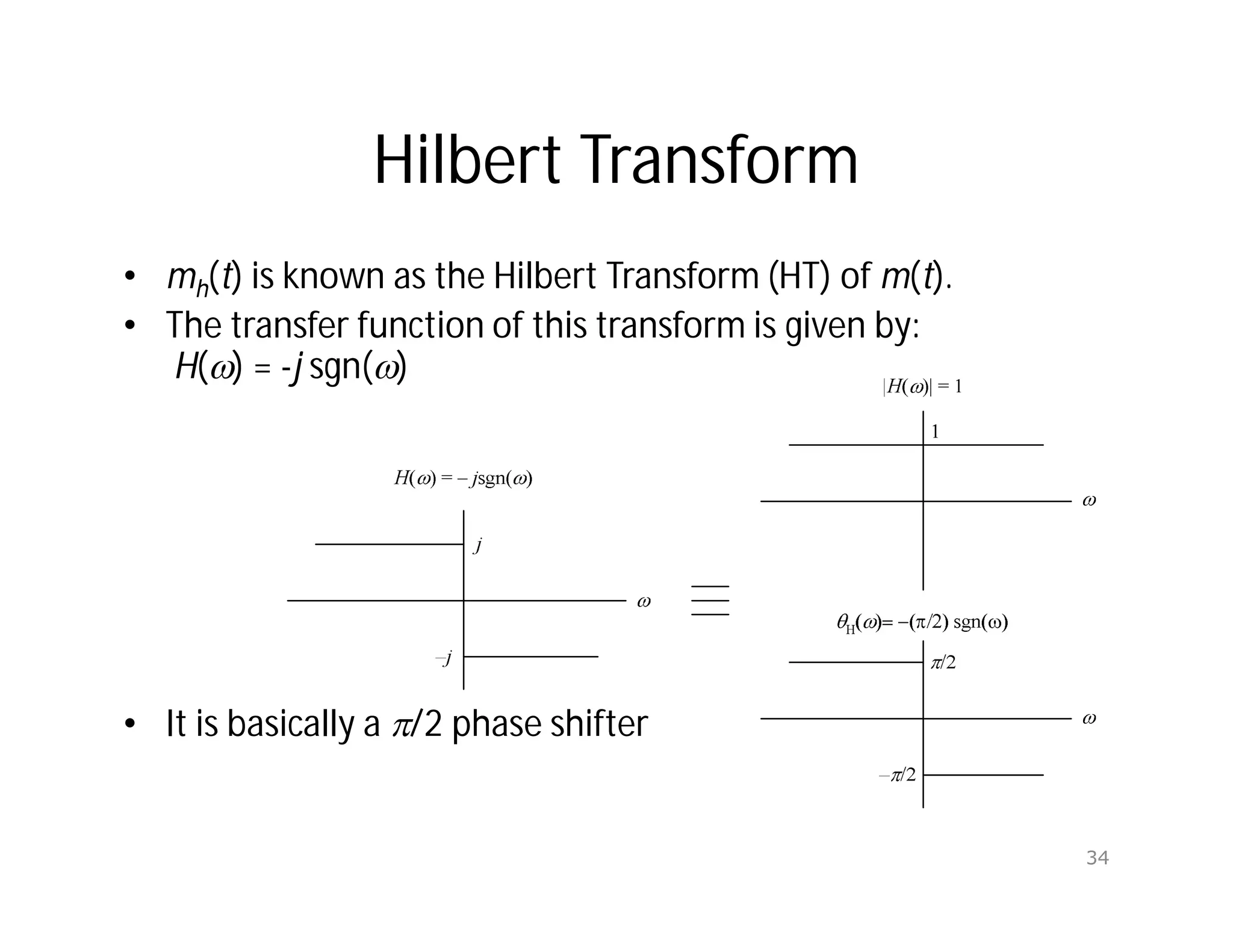
• mh(t) is known as the Hilbert Transform (HT) of m(t).
• The transfer function of this transform is given by:
H() = -j sgn()
• It is basically a /2 phase shifter
34

35. Hilbert Transform of cos(ct)
cos(ct) ↔  ( – c) + ( + c)]
HT[cos(ct)] ↔ -j sgn()  ( – c) + ( + c)]
= j sgn()  ( – c)  ( + c)]
= j  ( – c) + ( + c)]
= j  ( + c) - ( - c)] ↔ sin(ct)
Which is expected since:
cos(ct-/2) = sin(ct)
35

36. Time-Domain Operation for Hilbert
Transformation
For Hilbert Transformation H() = -j sgn().
What is h(t)?
sgn(t) ↔ 2/(j) [From FT table]
2/(jt) ↔ 2 sgn(-) [symmetry]
1/( t) ↔ -j sgn()
Since Mh() = - j M()∙sgn() = H() ∙ M()
Then












d
t
m
t
m
t
t
mh
)
(
1
)
(
*
1
)
(
36

37. )
sin(
)
(
)
cos(
)
(
)
(
2
1
)
(
2
1
)
(
2
1
)
(
2
1
)
(
)
sin(
)
(
)
cos(
)
(
)
(
2
1
)
(
2
1
)
(
2
1
)
(
2
1
)
(
t
t
m
t
t
m
e
t
jm
e
t
m
e
t
jm
e
t
m
t
g
t
t
m
t
t
m
e
t
jm
e
t
m
e
t
jm
e
t
m
t
g
C
h
C
t
j
h
t
j
t
j
h
t
j
LSB
C
h
C
t
j
h
t
j
t
j
h
t
j
USB
C
C
C
C
C
C
C
C




























)
(
)
(
)
(
)
(
)
(
)
(
C
C
LSB
C
C
USB
M
M
G
M
M
G






















t
j
t
j
LSB
t
j
t
j
USB
C
C
C
C
e
t
m
e
t
m
t
g
e
t
m
e
t
m
t
g




)
(
)
(
)
(
)
(
)
(
)
(










Finally …
37

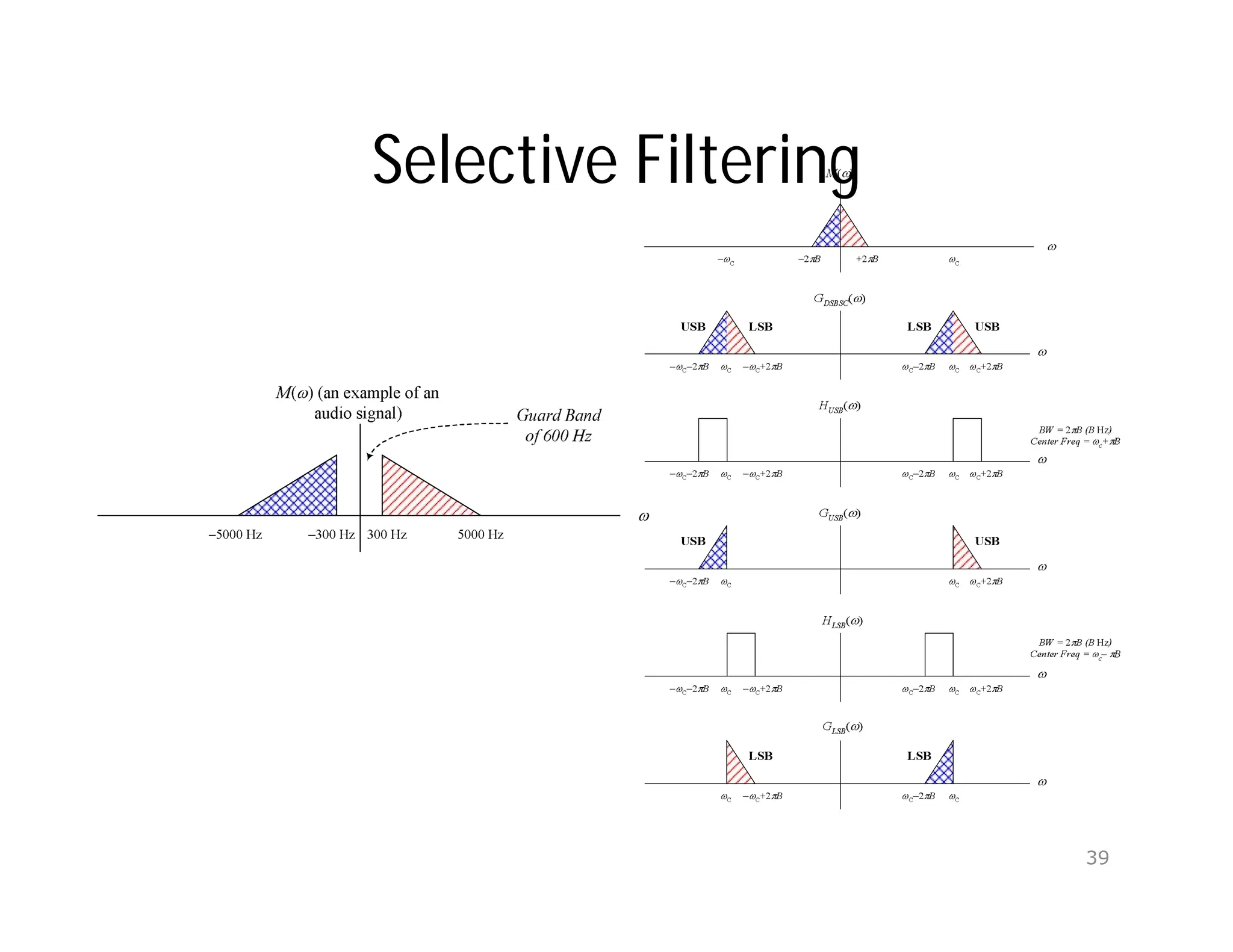
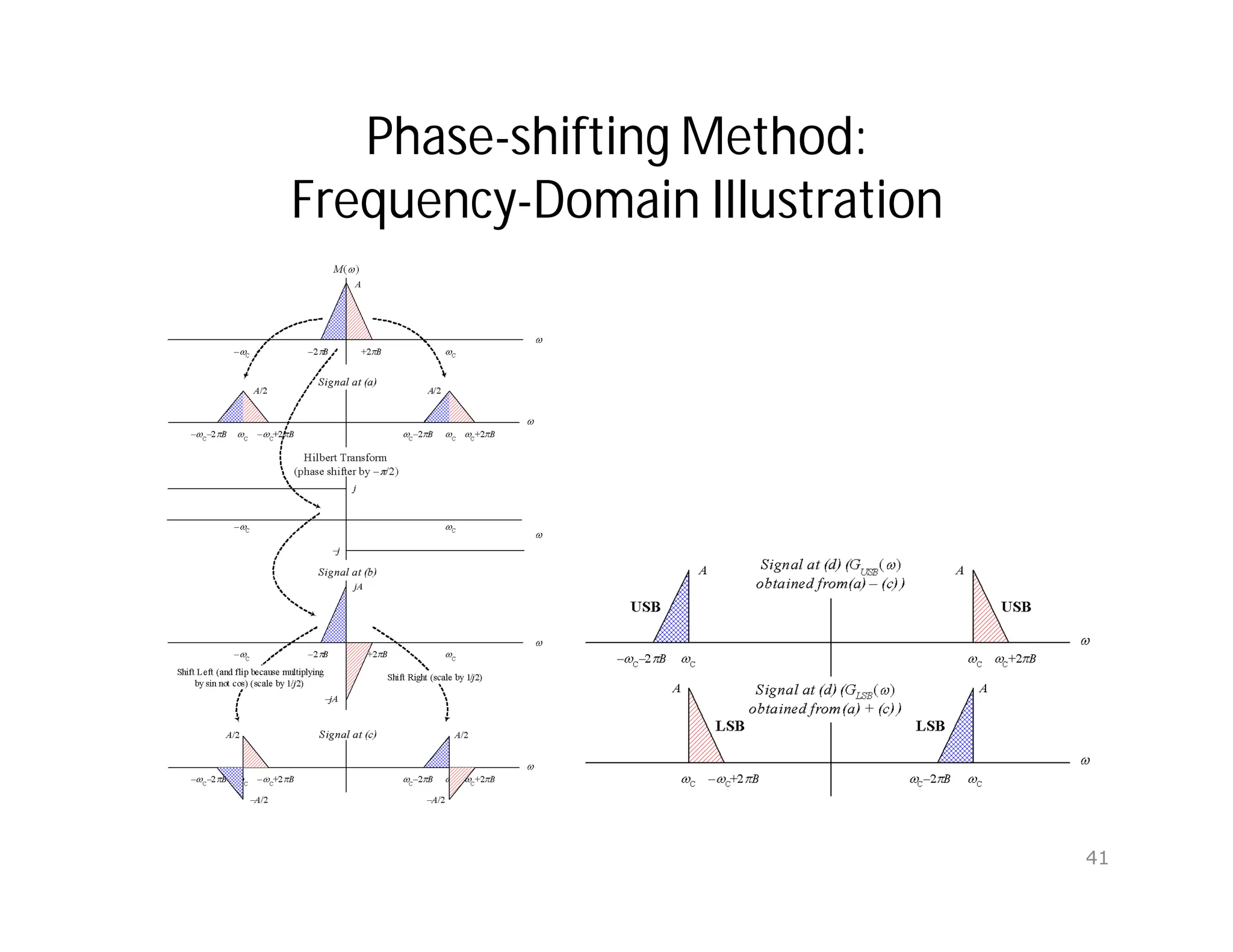
38. Generation of SSB
• Selective Filtering Method
Realization based on spectrum analysis
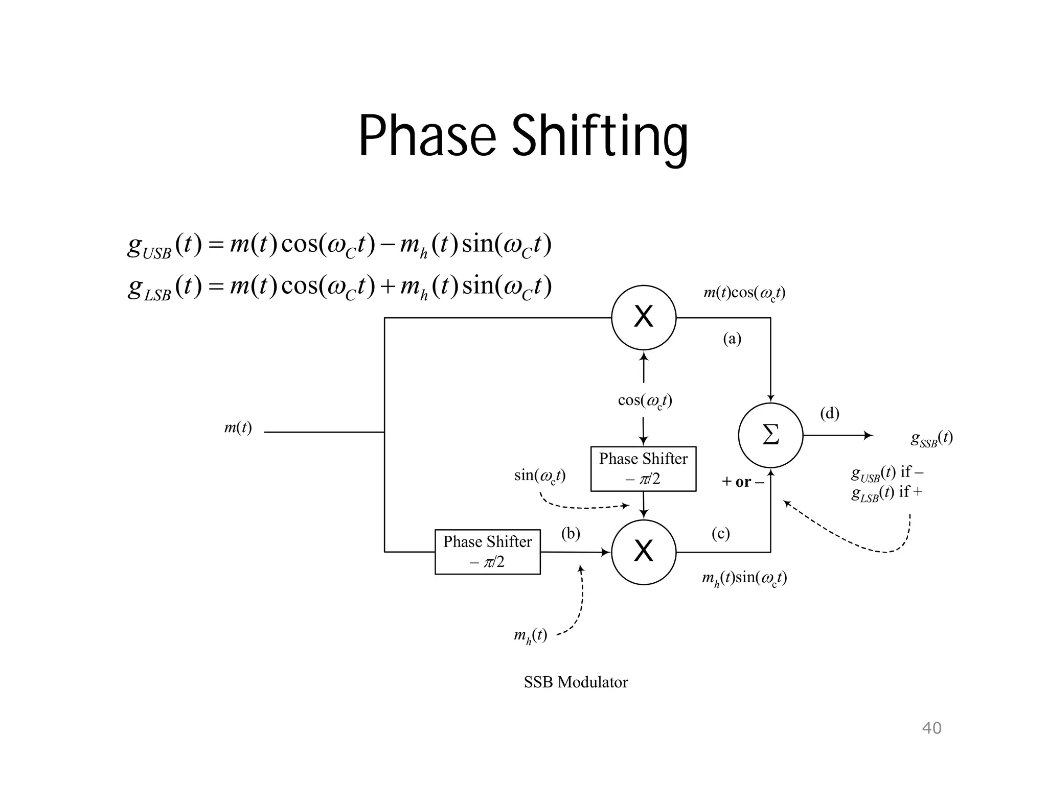
• Phase-Shift Method
Realization based on time-domain expression
of the modulated signal
38

39. Selective Filtering
39

40. Phase Shifting
)
sin(
)
(
)
cos(
)
(
)
(
)
sin(
)
(
)
cos(
)
(
)
(
t
t
m
t
t
m
t
g
t
t
m
t
t
m
t
g
C
h
C
LSB
C
h
C
USB








X
cos( ct)
SSB Modulator
X
sin( ct)
Phase Shifter
– /2
Phase Shifter
– /2
m(t)
mh
(t)
mh
(t)sin( c
t)
m(t)cos( ct)
gSSB
(t)
gUSB(t) if –
gLSB(t) if +
+ or –
(a)
(b) (c)
(d)
40

41. Phase-shifting Method:
Frequency-Domain Illustration
41

42. SSB Demodulation (Coherent)
)
(
2
1
Output
LPF
)
2
sin(
)
(
2
1
)]
2
cos(
1
)[
(
2
1
)
cos(
)
(
)
sin(
)
(
)
cos(
)
(
)
(
t
m
t
t
m
t
t
m
t
t
g
t
t
m
t
t
m
t
g
C
h
C
C
SSB
C
h
C
SSB











42

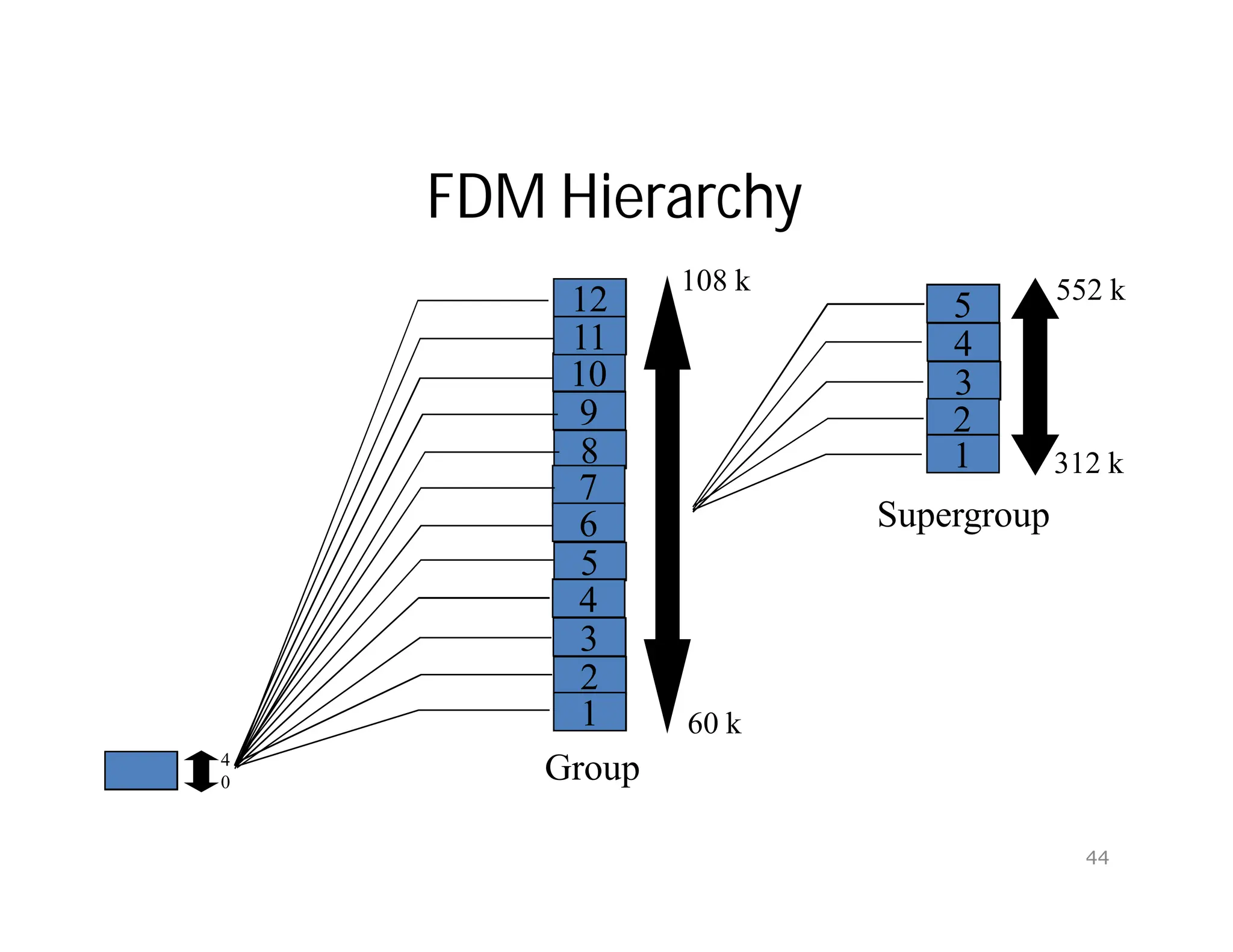
43. FDM in Telephony
• FDM is done in stages
– Reduce number of carrier frequencies
– More practical realization of filters
• Group: 12 voice channels  4 kHz = 48 kHz
occupy the band 60-108 kHz
• Supergroup: 5 groups  48 kHz = 240 kHz
occupy the band 312-552
• Mastergroup: 10 S-G  240 kHz = 2400 kHz
occupy the band 564-3084 kHz
43

44. FDM Hierarchy
4
0
5
4
3
2
1
10
9
8
7
6
5
4
3
2
1
11
12
60 k
108 k
312 k
552 k
Group
Supergroup
44

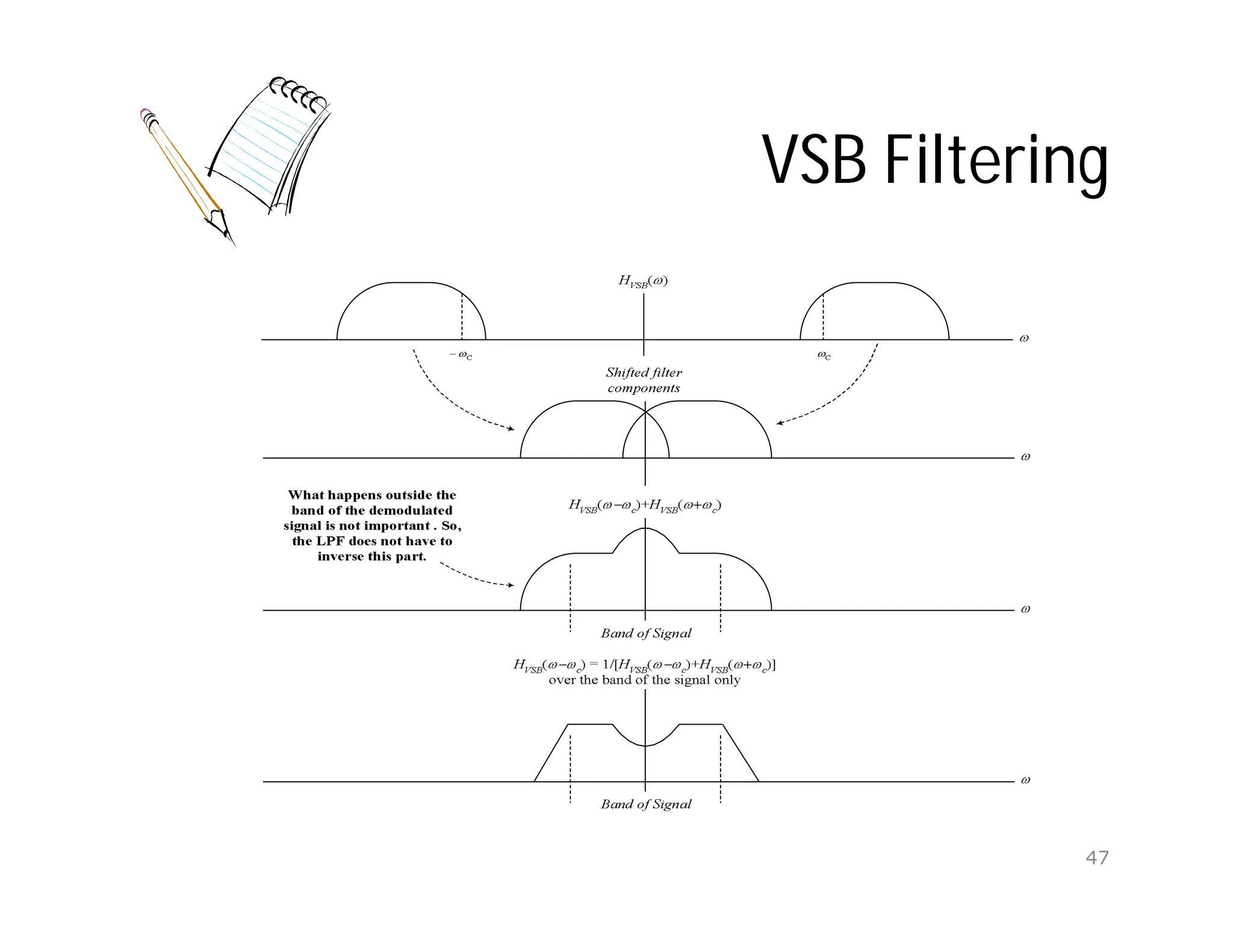
45. Vestigial Side Band Modulation (VSB)
• What if we want to generate SSB using
selective filtering but there is no guard band
between the two sides?
We will filter-in a vestige of the other band.
• Can we still recover our message, without
distortion, after demodulation?
Yes. If we use a proper LPF.
45

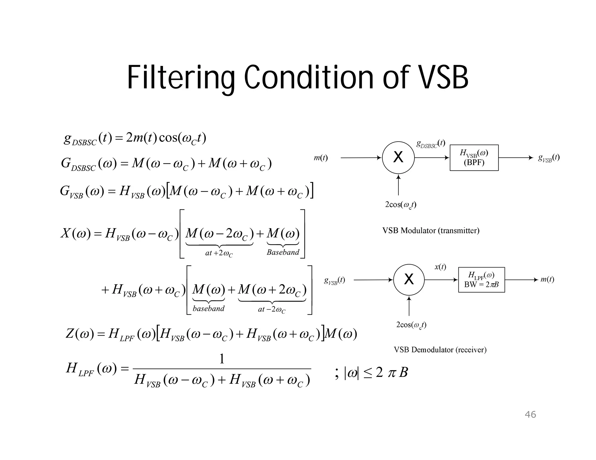
46. Filtering Condition of VSB
)
cos(
)
(
2
)
( t
t
m
t
g C
DSBSC 

)
(
)
(
)
( C
C
DSBSC M
M
G 



 



 
)
(
)
(
)
(
)
( C
C
VSB
VSB M
M
H
G 




 













































C
C
at
C
baseband
C
VSB
Baseband
at
C
C
VSB
M
M
H
M
M
H
X













2
2
)
2
(
)
(
)
(
)
(
)
2
(
)
(
)
(
  )
(
)
(
)
(
)
(
)
( 





 M
H
H
H
Z C
VSB
C
VSB
LPF 



)
(
)
(
1
)
(
C
VSB
C
VSB
LPF
H
H
H








 ; || ≤ 2  B
46

47. VSB Filtering
47

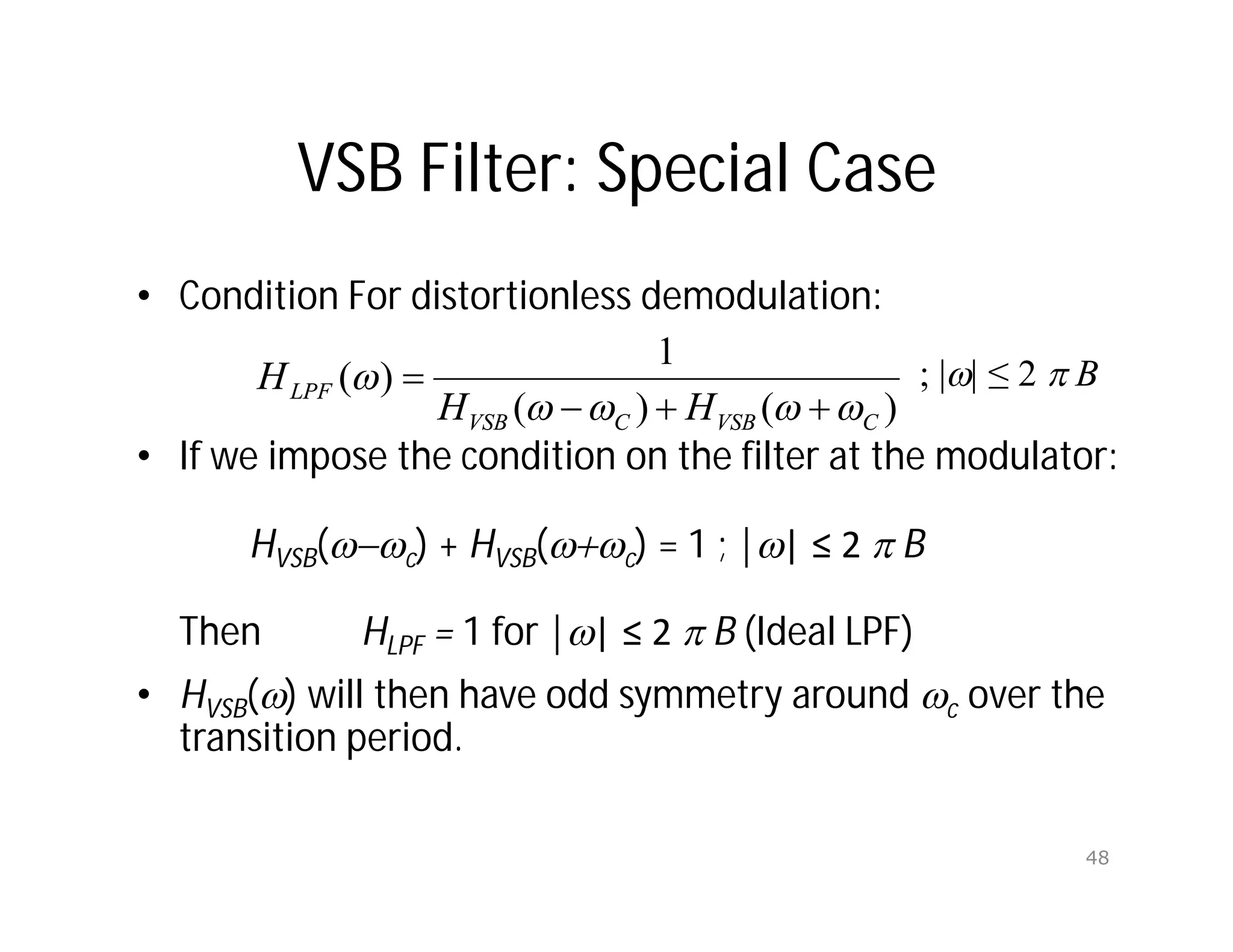
48. VSB Filter: Special Case
• Condition For distortionless demodulation:
• If we impose the condition on the filter at the modulator:
HVSB(-c) + HVSB(+c) = 1 ; || ≤ 2  B
Then HLPF = 1 for || ≤ 2  B (Ideal LPF)
• HVSB() will then have odd symmetry around c over the
transition period.
)
(
)
(
1
)
(
C
VSB
C
VSB
LPF
H
H
H








 ; || ≤ 2  B
48

49. 49

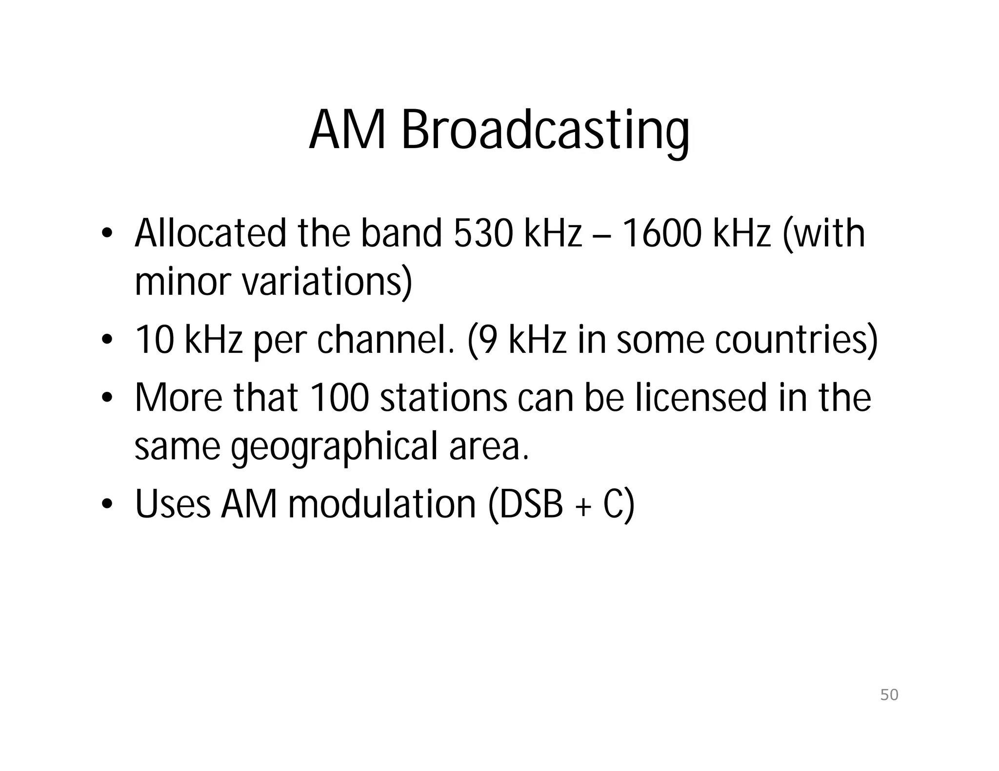
50. AM Broadcasting
• Allocated the band 530 kHz – 1600 kHz (with
minor variations)
• 10 kHz per channel. (9 kHz in some countries)
• More that 100 stations can be licensed in the
same geographical area.
• Uses AM modulation (DSB + C)
50

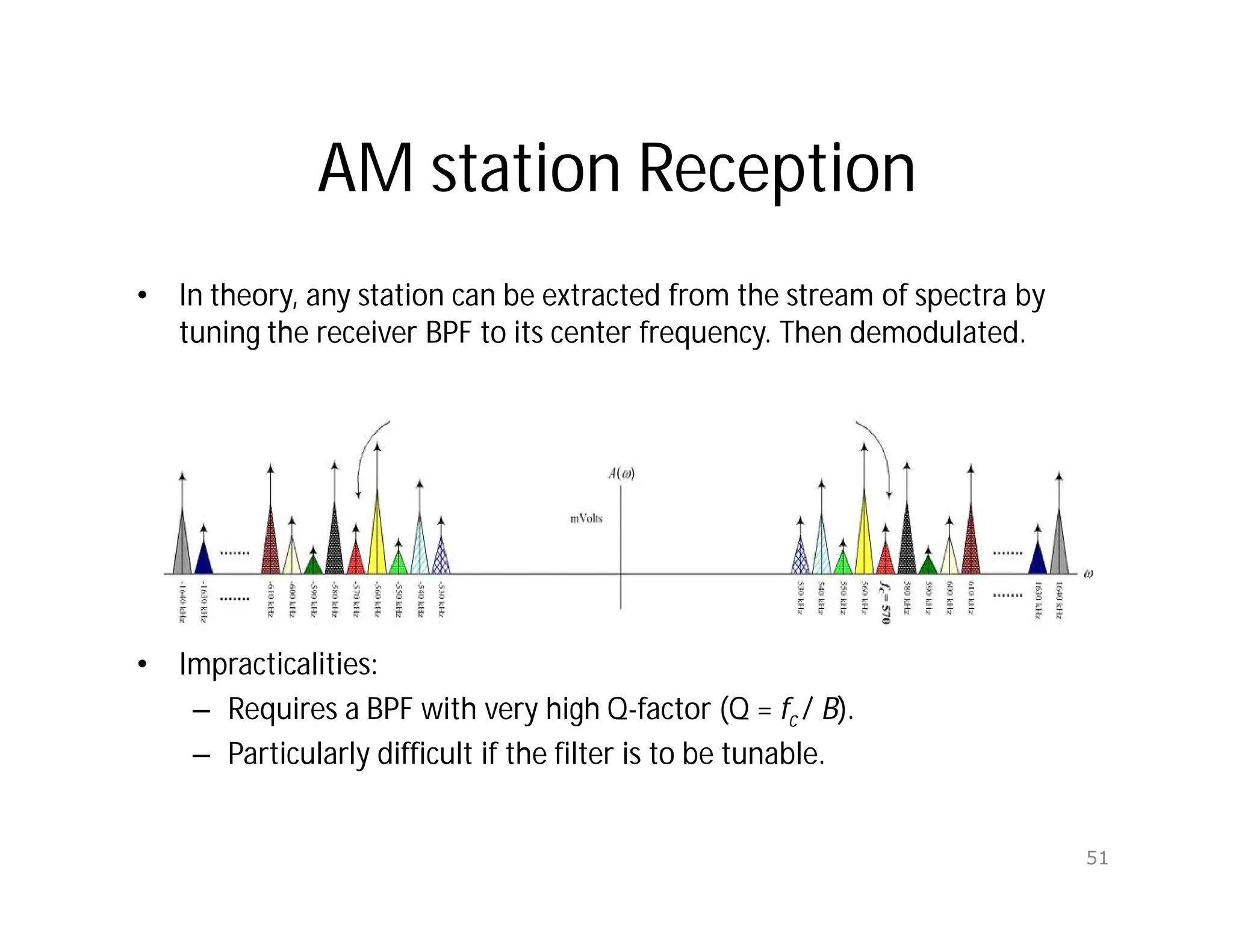
51. AM station Reception
• In theory, any station can be extracted from the stream of spectra by
tuning the receiver BPF to its center frequency. Then demodulated.
• Impracticalities:
– Requires a BPF with very high Q-factor (Q = fc / B).
– Particularly difficult if the filter is to be tunable.
51