verilog

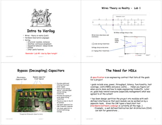
1. Intro to Verilog
• Wires – theory vs reality (Lab1)
• Hardware Description Languages
• Verilog
-- structural: modules, instances
-- dataflow: continuous assignment
-- sequential behavior: always blocks
-- pitfalls
-- other useful features
6.111 Fall 2017 1
Lecture 3
Reminder: Lab #1 due by 9pm tonight
Wires Theory vs Reality - Lab 1
6.111 Fall 2017 Lecture 3 2
Wires have inductance and
resistance
‫ܮ‬
ௗ௜
ௗ௧
noise during transitions
Voltage drop across wires
LC ringing after transitions
30-50mv voltage drop in chip
power
supply
noise
Bypass (Decoupling) Capacitors
6.111 Fall 2017 Lecture 3 3
Bypass capacitor
0.1uf typical
• Provides additional
filtering from main
power supply
• Used as local energy
source – provides peak
current during
transitions
• Provided decoupling of
noise spikes during
transitions
• Placed as close to the IC
as possible.
• Use small capacitors for
high frequency response.
• Use large capacitors to
localize bulk energy
storage
Electrolytic
Capacitor 10uf
Through hole PCB (ancient) shown for clarity.
The Need for HDLs
A specification is an engineering contract that lists all the goals
for a project:
• goals include area, power, throughput, latency, functionality, test
coverage, costs (NREs and piece costs), … Helps you figure out
when you’re done and how to make engineering tradeoffs. Later
on, goals help remind everyone (especially management) what was
agreed to at the outset!
• top-down design: partition the project into modules with well-
defined interfaces so that each module can be worked on by a
separate team. Gives the SW types a head start too!
(Hardware/software codesign is currently all the rage…)
• Example – a well defined Instruction Set Architecture (ISA)
can last for generations …
6.111 Fall 2017 4
Lecture 3

2. The Need for HDLs (cont’d.)
A behavioral model serves as an executable functional
specification that documents the exact behavior of all the
individual modules and their interfaces. Since one can run
tests, this model can be refined and finally verified through
simulation.
We need a way to talk about what hardware should do without
actually designing the hardware itself, i.e., we need to
separate behavior from implementation. We need a
Hardware Description Language
If we were then able to synthesize an implementation directly
from the behavioral model, we’d be in good shape!
6.111 Fall 2017 5
Lecture 3
Using an HDL description
So, we have an executable functional specification that
• documents exact behavior of all the modules and their
interfaces
• can be tested & refined until it does what we want
An HDL description is the first step in a mostly automated
process to build an implementation directly from the
behavioral model
Logic Synthesis Place & route
HDL
description
Gate
netlist
CPLD
FPGA
Stdcell ASIC
• HDL logic
• map to target library (LUTs)
• optimize speed, area
• create floor plan blocks
• place cells in block
• route interconnect
• optimize (iterate!)
Physical design
Functional design
6.111 Fall 2017 6
Lecture 3
A Tale of Two HDLs
VHDL Verilog
ADA-like verbose syntax, lots of
redundancy (which can be good!)
C-like concise syntax
Extensible types and simulation
engine. Logic representations are
not built in and have evolved with
time (IEEE-1164).
Built-in types and logic
representations. Oddly, this led
to slightly incompatible simulators
from different vendors.
Design is composed of entities
each of which can have multiple
architectures. A configuration
chooses what architecture is
used for a given instance of an
entity.
Design is composed of modules.
Behavioral, dataflow and
structural modeling.
Synthesizable subset...
Behavioral, dataflow and
structural modeling.
Synthesizable subset...
Harder to learn and use, not
technology-specific, DoD mandate
Easy to learn and use, fast
simulation, good for hardware
design
6.111 Fall 2017 7
Lecture 3
Universal Constraint File - UCF
• Text file containing the mapping from a device independent HDL
circuit net to the physical I/O pin. This allows Verilog (HDL) to
be device independent.
– Assigns bit 35 of the signal ram0_data to pin ab25 on the IC
– Specifies the i/o driver configured for fast slew rate with 3.3V LVTTL level
– Specifies drive strength of 12mA
• Constraints may also include timing constraints.
• Don’t worry – all constraints for the labkit have been defined
• For Vivado, xdc file are used (Xilinx Design Constraint)
{PACKAGE_PIN H17 IOSTANDARD LVCMOS33 } [get_ports { LED[0] }];
– LED[0] is 3.3C CMOS being driven by IC Package H pin 17
6.111 Fall 2017 Lecture 3 8
net "ram0_data<35>" loc="ab25" | fast | iostandard=lvdci_33 | drive=12;

3. Verilog data values
Since we’re describing hardware, we’ll need to represent the
values that can appear on wires. Verilog uses a 4-valued logic:
Value Meaning
0 Logic zero, “low”
1 Logic one, “high”
Z or ? High impedance (tri-state buses)
X Unknown value (simulation)
“X” is used by simulators when a wire hasn’t been initialized to a
known value or when the predicted value is an illegitimate logic
value (e.g., due to contention on a tri-state bus).
Verilog also has the notion of “drive strength” but we can safely
ignore this feature for our purposes.
6.111 Fall 2017 9
Lecture 3
Numeric Constants
Constant values can be specified with a specific width and radix:
123 // default: decimal radix, unspecified width
‘d123 // ‘d = decimal radix
‘h7B // ‘h = hex radix
‘o173 // ‘o = octal radix
‘b111_1011 // ‘b = binary radix, “_” are ignored
‘hxx // can include X, Z or ? in non-decimal constants
16’d5 // 16-bit constant ‘b0000_0000_0000_0101
11’h1X? // 11-bit constant ‘b001_XXXX_ZZZZ
By default constants are unsigned and will be extended with 0’s
on left if need be (if high-order bit is X or Z, the extended bits
will be X or Z too). You can specify a signed constant as follows:
8’shFF // 8-bit twos-complement representation of -1
To be absolutely clear in your intent it’s usually best to explicitly
specify the width and radix.
6.111 Fall 2017 10
Lecture 3
Wires
We have to provide declarations* for all our named wires (aka
“nets”). We can create buses – indexed collections of wires – by
specifying the allowable range of indices in the declaration:
wire a,b,z; // three 1-bit wires
wire [31:0] memdata; // a 32-bit bus
wire [7:0] b1,b2,b3,b4; // four 8-bit buses
wire [W-1:0] input; // parameterized bus
Note that [0:7] and [7:0] are both legitimate but it pays to
develop a convention and stick with it. Common usage is
[MSB:LSB] where MSB > LSB; usually LSB is 0. Note that we can
use an expression in our index declaration but the expression’s
value must be able to be determined at compile time. We can also
build unnamed buses via concatenation:
{b1,b2,b3,b4} // 32-bit bus, b1 is [31:24], b2 is [23:16], …
{4{b1[3:0]},16’h0000} // 32-bit bus, 4 copies of b1[3:0], 16 0’s
* Actually by default undeclared identifiers refer to a 1-bit wire, but this means typos get
you into trouble. Specify “`default_nettype none” at the top of your source files to avoid
this bogus behavior.
6.111 Fall 2017 11
Lecture 3
General tips for less bugs
• Add `default_nettype none at the top of your source files.This
prevents ISE/Vivado from inferring wires from module
instantiations and forces you to explicitly declare wires and regs
(and their widths) before using them [May need to comment out
for Modelsim.]
• Read synthesis warnings. Most can be can be ignored but a few
are important: port width mismatches, unused wires, naming
errors, etc
• Common errors:
– Multiple sources
– Unmatch constraints
6.111 Fall 2017 Lecture 1 12

4. Basic building block: modules
// 2-to-1 multiplexer with dual-polarity outputs
module mux2(input a,b,sel, output z,zbar);
wire selbar,z1,z2; // wires internal to the module
// order doesn’t matter – all statements are
// executed concurrently!
not i1(selbar,sel); // inverter, name is “i1”
and a1(z1,a,selbar); // port order is (out,in1,in2,…)
and a2(z2,b,sel);
or o1(z,z1,z2);
not i2(zbar,z);
endmodule
In Verilog we design modules, one of which will be identified as
our top-level module. Modules usually have named, directional
ports (specified as input, output or inout) which are used to
communicate with the module.
In this example the module’s behavior is specified using Verilog’s
built-in Boolean modules: not, buf, and, nand, or, nor, xor,
xnor. Just say no! We want to specify behavior, not implementation!
Don’t forget this “;”
6.111 Fall 2017 13
Lecture 3
z
zbar
sel
b
a
z2
z1
selbar
Continuous assignments
// 2-to-1 multiplexer with dual-polarity outputs
module mux2(input a,b,sel, output z,zbar);
// again order doesn’t matter (concurrent execution!)
// syntax is “assign LHS = RHS” where LHS is a wire/bus
// and RHS is an expression
assign z = sel ? b : a;
assign zbar = ~z;
endmodule
If we want to specify a behavior equivalent to combinational logic,
use Verilog’s operators and continuous assignment statements:
Conceptually assign’s are evaluated continuously, so whenever a
value used in the RHS changes, the RHS is re-evaluated and the
value of the wire/bus specified on the LHS is updated.
This type of execution model is called “dataflow” since evaluations
are triggered by data values flowing through the network of wires
and operators.
6.111 Fall 2017 14
Lecture 3
Boolean operators
• Bitwise operators perform bit-oriented operations on vectors
• ~(4’b0101) = {~0,~1,~0,~1} = 4’b1010
• 4’b0101 & 4’b0011 = {0&0, 1&0, 0&1, 1&1} = 4’b0001
• Reduction operators act on each bit of a single input vector
• &(4’b0101) = 0 & 1 & 0 & 1 = 1’b0
• Logical operators return one-bit (true/false) results
• !(4’b0101) = 1’b0
~a NOT
a & b AND
a | b OR
a ^ b XOR
a ~^ b
a ^~ b
XNOR
Bitwise Logical
!a NOT
a && b AND
a || b OR
a == b
a != b
[in]equality
returns x when x
or z in bits. Else
returns 0 or 1
a === b
a !== b
case
[in]equality
returns 0 or 1
based on bit by bit
comparison
&a AND
~&a NAND
|a OR
~|a NOR
^a XOR
~^a
^~a
XNOR
Reduction
Note distinction between ~a and !a
when operating on multi-bit values
6.111 Fall 2017 15
Lecture 3
Boolean operators
• ^ is NOT exponentiation (**)
• Logical operator with z and x
• 4'bz0x1 === 4'bz0x1 = 1 4'bz0x1 === 4'bz001 = 0
• Bitwise operator with z and x
• 4'b0001 & 4'b1001 = 0001 4'b1001 & 4'bx001 = x001
~a NOT
a & b AND
a | b OR
a ^ b XOR
a ~^ b
a ^~ b
XNOR
Bitwise Logical
!a NOT
a && b AND
a || b OR
a == b
a != b
[in]equality
returns x when x
or z in bits. Else
returns 0 or 1
a === b
a !== b
case
[in]equality
returns 0 or 1
based on bit by bit
comparison
&a AND
~&a NAND
|a OR
~|a NOR
^a XOR
~^a
^~a
XNOR
Reduction
Note distinction between ~a and !a
when operating on multi-bit values
6.111 Fall 2017 16
Lecture 3

5. Integer Arithmetic
• Verilog’s built-in arithmetic makes a 32-bit adder easy:
• A 32-bit adder with carry-in and carry-out:
module add32
(input[31:0] a, b,
output[31:0] sum);
assign sum = a + b;
endmodule
module add32_carry
(input[31:0] a,b,
input cin,
output[31:0] sum,
output cout);
assign {cout, sum} = a + b + cin;
endmodule
concatenation
6.111 Fall 2017 17
Lecture 3
Other operators
a ? b : c If a then b else c
Conditional
-a negate
a + b add
a - b subtract
a * b multiply
a / b divide
a % b modulus
a ** b exponentiate
a << b logical left shift
a >> b logical right shift
a <<< b arithmetic left shift
a >>> b arithmetic right shift
Arithmetic
a > b greater than
a >= b greater than or equal
a < b Less than
a <= b Less than or equal
Relational
6.111 Fall 2017 18
Lecture 3
Hierarchy: module instances
// 4-to-1 multiplexer
module mux4(input d0,d1,d2,d3, input [1:0] sel, output z);
wire z1,z2;
// instances must have unique names within current module.
// connections are made using .portname(expression) syntax.
// once again order doesn’t matter…
mux2 m1(.sel(sel[0]),.a(d0),.b(d1),.z(z1)); // not using zbar
mux2 m2(.sel(sel[0]),.a(d2),.b(d3),.z(z2));
mux2 m3(.sel(sel[1]),.a(z1),.b(z2),.z(z));
// could also write “mux2 m3(z1,z2,sel[1],z,)” NOT A GOOD IDEA!
endmodule
Our descriptions are often hierarchical, where a module’s
behavior is specified by a circuit of module instances:
Connections to module’s ports are made using a syntax that specifies
both the port name and the wire(s) that connects to it, so ordering of
the ports doesn’t have to be remembered (“explicit”).
This type of hierarchical behavioral model is called “structural” since
we’re building up a structure of instances connected by wires. We
often mix dataflow and structural modeling when describing a module’s
behavior.
6.111 Fall 2017 19
Lecture 3
Parameterized modules
// 2-to-1 multiplexer, W-bit data
module mux2 #(parameter W=1) // data width, default 1 bit
(input [W-1:0] a,b,
input sel,
output [W-1:0] z);
assign z = sel ? b : a;
assign zbar = ~z;
endmodule
// 4-to-1 multiplexer, W-bit data
module mux4 #(parameter W=1) // data width, default 1 bit
(input [W-1:0] d0,d1,d2,d3,
input [1:0] sel,
output [W-1:0] z);
wire [W-1:0] z1,z2;
mux2 #(.W(W)) m1(.sel(sel[0]),.a(d0),.b(d1),.z(z1));
mux2 #(.W(W)) m2(.sel(sel[0]),.a(d2),.b(d3),.z(z2));
mux2 #(.W(W)) m3(.sel(sel[1]),.a(z1),.b(z2),.z(z));
endmodule
could be an expression evaluable at compile time;
if parameter not specified, default value is used
6.111 Fall 2017 20
Lecture 3

6. Sequential behaviors
// 4-to-1 multiplexer
module mux4(input a,b,c,d, input [1:0] sel, output reg z,zbar);
always @(*) begin
if (sel == 2’b00) z = a;
else if (sel == 2’b01) z = b;
else if (sel == 2’b10) z = c;
else if (sel == 2’b11) z = d;
else z = 1’bx; // when sel is X or Z
// statement order matters inside always blocks
// so the following assignment happens *after* the
// if statement has been evaluated
zbar = ~z;
end
endmodule
There are times when we’d like to use sequential semantics and
more powerful control structures – these are available inside
sequential always blocks:
always @(*) blocks are evaluated whenever any value used inside
changes. Equivalently we could have written
always @(a, b, c, d, sel) begin … end // careful, prone to error!
6.111 Fall 2017 21
Lecture 3
reg vs wire
We’ve been using wire declarations when naming nets (ports are
declared as wires by default). However nets appearing on the
LHS of assignment statements inside of always blocks must be
declared as type reg.
I don’t know why Verilog has this rule! I think it’s because
traditionally always blocks were used for sequential logic (the
topic of next lecture) which led to the synthesis of hardware
registers instead of simply wires. So this seemingly
unnecessary rule really supports historical usage – the
declaration would help the reader distinguish registered
values from combinational values.
We can add the reg keyword to output or inout ports (we
wouldn’t be assigning values to input ports!), or we can declare
nets using reg instead of wire.
output reg [15:0] result // 16-bit output bus assigned in always block
reg flipflop; // declaration of 1-bit net of type reg
6.111 Fall 2017 22
Lecture 3
Case statements
// 4-to-1 multiplexer
module mux4(input a,b,c,d, input [1:0] sel, output reg z,zbar);
always @(*) begin
case (sel)
2’b00: z = a;
2’b01: z = b;
2’b10: z = c;
2’b11: z = d;
default: z = 1’bx; // in case sel is X or Z
endcase
zbar = ~z;
end
endmodule
Chains of if-then-else statements aren’t the best way to indicate
the intent to provide an alternative action for every possible
control value. Instead use case:
case looks for an exact bit-by-bit match of the value of the case
expression (e.g., sel) against each case item, working through the
items in the specified order. casex/casez statements treat X/Z
values in the selectors as don’t cares when doing the matching
that determines which clause will be executed.
6.111 Fall 2017 23
Lecture 3
Unintentional creation of state
// 3-to-1 multiplexer ????
module mux3(input a,b,c, input [1:0] sel, output reg z);
always @(*) begin
case (sel)
2’b00: z = a;
2’b01: z = b;
2’b10: z = c;
// if sel is 2’b11, no assignment to z!!??
endcase
end
endmodule
Suppose there are multiple execution paths inside an always
block, i.e., it contains if or case statements, and that on some
paths a net is assigned and on others it isn’t.
So sometimes z changes and sometimes it doesn’t (and hence
keeps its old value). That means the synthesized hardware has to
have a way of remembering the state of z (i.e., it’s old value) since
it’s no longer just a combinational function of sel, a, b, and c. Not
what was intended here. More on this in next lecture.
6.111 Fall 2017 24
Lecture 3
00
sel
z
01
10
a
b
c
2
D Q
G
sel[1]
sel[0]

7. Keeping logic combinational
// 3-to-1 multiplexer
module mux3(input a,b,c, input [1:0] sel, output reg z);
always @ (*) begin
z = 1’bx; // a second assignment may happen below
case (sel)
2’b00: z = a;
2’b01: z = b;
2’b10: z = c;
default: z = 1’bx;
endcase
end
endmodule
To avoid the unintentional creation of state, ensure that each
variable that’s assigned in an always block always gets assigned a
new value at least once on every possible execution path.
It’s good practice when writing combinational always blocks to
provide a default: clause for each case statement and an else
clause for each if statement.
6.111 Fall 2017 25
Lecture 3
Use one or
the other
Other useful Verilog features
• Additional control structures: for, while, repeat, forever
• Procedure-like constructs: functions, tasks
• One-time-only initialization: initial blocks
• Compile-time computations: generate, genvar
• System tasks to help write simulation test jigs
– Stop the simulation: $finish(…)
– Print out text, values: $display(…)
– Initialize memory from a file: $readmemh(…), $readmemb(…)
– Capture simulation values: $dumpfile(…), $dumpvars(…)
– Explicit time delays (simulation only!!!!) : #nnn
• Compiler directives
– Macro definitions: `define
– Conditional compilation: `ifdef, …
– Control simulation time units: `timescale
– No implicit net declarations: `default_nettype none
6.111 Fall 2017 26
Lecture 3
Defining Processor ALU in 5 mins
• Modularity is essential to the success of large designs
• High-level primitives enable direct synthesis of behavioral descriptions
(functions such as additions, subtractions, shifts (<< and >>), etc.
A[31:0] B[31:0]
+ - *
0 1 0 1
32’d1 32’d1
00 01 10
R[31:0]
F[0]
F[2:1]
F[2:0]
Example: A 32-bit ALU
F2 F1 F0
0 0 0
0 0 1
0 1 0
0 1 1
1 0 X
Function
A + B
A + 1
A - B
A - 1
A * B
Function Table
6.111 Fall 2017 27
Lecture 3
Module Definitions
2-to-1 MUX 3-to-1 MUX
32-bit Adder
32-bit Subtracter
16-bit Multiplier
module mux32two
(input [31:0] i0,i1,
input sel,
output [31:0] out);
assign out = sel ? i1 : i0;
endmodule
module mux32three
(input [31:0] i0,i1,i2,
input [1:0] sel,
output reg [31:0] out);
always @ (i0 or i1 or i2 or sel)
begin
case (sel)
2’b00: out = i0;
2’b01: out = i1;
2’b10: out = i2;
default: out = 32’bx;
endcase
end
endmodule
module add32
(input [31:0] i0,i1,
output [31:0] sum);
assign sum = i0 + i1;
endmodule
module sub32
(input [31:0] i0,i1,
output [31:0] diff);
assign diff = i0 - i1;
endmodule
module mul16
(input [15:0] i0,i1,
output [31:0] prod);
// this is a magnitude multiplier
// signed arithmetic later
assign prod = i0 * i1;
endmodule
6.111 Fall 2017 28
Lecture 3

8. Top-Level ALU Declaration
• Given submodules:
• Declaration of the ALU Module:
module mux32two(i0,i1,sel,out);
module mux32three(i0,i1,i2,sel,out);
module add32(i0,i1,sum);
module sub32(i0,i1,diff);
module mul16(i0,i1,prod);
A[31:0] B[31:0]
+ - *
0 1 0 1
32’d1 32’d1
00 01 10
R[31:0]
F[0]
F[2:1]
F[2:0]
module
names
(unique)
instance
names
corresponding
wires/regs in
module alu
intermediate output nodes
alu
6.111 Fall 2017 29
Lecture 3
module alu
(input [31:0] a, b,
input [2:0] f,
output [31:0] r);
wire [31:0] addmux_out, submux_out;
wire [31:0] add_out, sub_out, mul_out;
mux32two adder_mux(b, 32'd1, f[0], addmux_out);
mux32two sub_mux(b, 32'd1, f[0], submux_out);
add32 our_adder(a, addmux_out, add_out);
sub32 our_subtracter(a, submux_out, sub_out);
mul16 our_multiplier(a[15:0], b[15:0], mul_out);
mux32three output_mux(add_out, sub_out, mul_out, f[2:1], r);
endmodule
Use Explicit Port Declarations
6.111 Fall 2017 Lecture 1 30
mux32two adder_mux(b, 32'd1, f[0], addmux_out);
mux32two adder_mux(,i0(b), .i1(32'd1),
.sel(f[0]), .out(addmux_out));
Order of the ports matters!
ModelSim/Testbench Introduction
module full_adder
(input a, b, cin,
output reg sum, cout);
always @(a or b or cin)
begin
sum = a ^ b ^ cin;
cout = (a & b) | (a & cin) | (b & cin);
end
Endmodule
module full_adder_4bit
( input[3:0] a, b,
input cin,
output [3:0] sum,
output cout),
wire c1, c2, c3;
// instantiate 1-bit adders
full_adder FA0(a[0],b[0], cin, sum[0], c1);
full_adder FA1(a[1],b[1], c1, sum[1], c2);
full_adder FA2(a[2],b[2], c2, sum[2], c3);
full_adder FA3(a[3],b[3], c3, sum[3], cout);
endmodule
Full Adder (1-bit) Full Adder (4-bit)
Testbench
ModelSim Simulation
module test_adder;
reg [3:0] a, b;
reg cin;
wire [3:0] sum;
wire cout;
full_adder_4bit dut(a, b, cin,
sum, cout);
initial
begin
a = 4'b0000;
b = 4'b0000;
cin = 1'b0;
#50;
a = 4'b0101;
b = 4'b1010;
// sum = 1111, cout = 0
#50;
a = 4'b1111;
b = 4'b0001;
// sum = 0000, cout = 1
#50;
a = 4'b0000;
b = 4'b1111;
cin = 1'b1;
// sum = 0000, cout = 1
#50;
a = 4'b0110;
b = 4'b0001;
// sum = 1000, cout = 0
end // initial begin
endmodule // test_adder
Courtesy of F. Honore, D. Milliner
FPGA Labkit
6.111 Fall 2017 Lecture 1 32
button_down, button_enter, … led[7:0], switch[7:0]
negative logic negative logic
Inputs and displays
16 alphanumeric display (10x4)

9. FPGA Labkit – User I/O
6.111 Fall 2017 Lecture 1 33
4 banks – 16 user i/p
NTSC Video/Audio
6.111 Fall 2017 Lecture 1 34
Video, audio, in/out
S-Video in/put
VGA, Serial, Keyboard, Mouse
6.111 Fall 2017 Lecture 1 35
VGA Serial port Keyboard, Mouse
Lab 2
• Lab 2 – Part A
– Labkit
– Modelsim
– ISE
– Impact
• Lab 2 – Part B
– Serial Communications
– Install Python 3 and pyserial
• Make sure you start early!
6.111 Fall 2017 Lecture 3 36