control systems nptel lecture 25

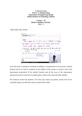
1. Control Systems
Prof. C. S. Shankar Ram
Department of Engineering Design
Indian Institute of Technology, Madras
Lecture – 25
Routh’s Stability Criterion
Part – 1
(Refer Slide Time: 00:20)
In the last class we looked at evaluation of stability, we learned that if we are given a transfer
function and if we want to comment on the stability of the system, we need to look at the
denominator polynomial of the transfer function and all the roots of the denominator
polynomial must be in the left of complex plane, which is the criteria for bibo stability.
We wanted to answer the question: if we have any system any generic system, how do we
essentially figure out when that system would be bibo stable.

2. (Refer Slide Time: 01:30)
We solved a problem where the plant transfer function was
P(s)=
1
s
2
+1
we saw that it has poles on the imaginary axis at ± j . So we know, if we give an input like
cost or sint , the output is going to become unbounded.
(Refer Slide Time: 01:52)

3. (Refer Slide Time: 02:00)
We wanted to design a unity negative feedback system. And, we tried with the proportional
controller and found out that the proportional controller could not help us there. When we
tried the PI controller, we ended up with a third order polynomial. Now, we have two
parameters that we can change and a third order polynomial. With this can we find out the
ranges of values of these parameters for which the close poles would lie in the left half
complex plane.
In general when would a polynomial be Hurwitz? If we consider a polynomial
D (s)=a0 s
n
+a1 s
n−1
+…+an ,
where all the coefficients a0 ,a1 …an are all real numbers. This polynomial is said to be
Hurwitz if all it is roots have negative real parts, In our discussion, we want the denominator
polynomial of the closed loop transfer function to be Hurwitz. Then we are assured that the
closed loop system is going to be stable. How do we evaluate whether a given polynomial
D (s) is going to be Hurwitz? This is the question we are going to answer.
Let us first consider a first order polynomial (n=1) .
D (s)=a0 s+a1

4. This would be Hurwitz when a0 ≠0,a1≠0, and both a0 and a1 have the same sign.
They can both be positive or both be negative. In this case the root is going to be
−a1
a0
. If
we want this real root to be negative then both the real numbers must be of the same sign.
Now, let us first consider a first order polynomial (n=2)
D (s)=a0 s
2
+a1 s+a2 .
It so turns out that this polynomial would be Hurwitz when a0 , a1 and a2 are all
nonzero and of the same sign. The roots are going to be in the left of complex plane. We can
tell this for sure even without calculating the roots.
Now let us go to n=3 . The polynomial becomes
D (s)=a0 s
3
+a1s
2
+a2 s+a3 .
There are four coefficients. For an n
th
order polynomial we are going to have n+1
coefficients. In any general, in any n
th
order polynomial if a0=1 , that is called as a
monic polynomial. That means that the coefficient of the highest order term is 1.
Now, for the roots to lie in the left of complex plane we still need a0, a1,a2 and a3 to be
non-zero and of the same sign. But for polynomials of order 3 and more that is only a
necessary condition. For polynomials of order 1 and 2, the necessary condition is also
sufficient but not far polynomials of order 3 and more. Let us demonstrate it through two
examples ok.

5. (Refer Slide Time: 09:49)
Let us consider the first polynomial to be
D1=s
3
+2s
2
+3s+1.
And the second polynomial the polynomial to be
D2=s
3
+2s
2
+s+3.
If we determine the roots of the above equations, we can see that, all the roots of D1 have
negative real parts and lie in the left of complex plane. And D2 has one root on the left of
complex plane and two roots in the right of complex plane.
The only change between D1 and D2 is the coefficient of s term and constant term
are interchanged. In these two polynomials all coefficients are nonzero and of the same sign.
But we see a drastic change in the way the roots of the two polynomials are distributed. We
can see that what was necessary and sufficient for polynomial till order 2 is not sufficient
here.
For sufficiency we construct the Routh’s array. The Routh’s array is constructed as shown
below.

6. (Refer Slide Time: 17:31)
s
n
a0 a2 a4 a6 …
s
n−1
a1 a3 a5 a7 …
s
n−2
b1 b2 b3 …
s
n−3
c1 c2 c3 …
⋮ ⋮ ⋮ ⋮
s
1 ⋮ ⋮
s
0
⋮
We write the column s
n
till s
0
and then we start filling in the first two rows of this array
with the coefficients of the polynomial which we are given in the order of the decreasing
powers as seen in the array. We fill the first two rows till the coefficients get exhausted. Then
we start calculating bi and ci terms.
Let us come to b1 . So, if we want to calculate matter any coefficient in any row we
consider the coefficients which are available in the two rows that are immediately above that
row. In this case b1 appears in the s
n−2
row. So, we consider the two rows immediately
above that which are s
n−1
and s
n
. Then b1 is calculated as
b1=
a1a2−a0 a3
a1
Similarly, b2=
a1a4−a0 a5
a1

7. c1=
b1 a3−a1b2
b1
c2=
b1 a5−a1b3
b1
We continue this process until we finish constructing the Routh’s array. Once we finish this
process, we look at the first column of the Routh’s array. The sufficiency condition is that
there should not be any sign changes in the first column of the Routh’s array for the
polynomial to be Hurwitz. That is that the number of sign changes in the first column of the
Routh’s array should be 0.
So for any general polynomial of order n with real coefficients, the necessary condition is that
all the coefficient must be non-zero and of the same sign. The sufficient condition is that the
first column of the Routh’s array should not have any sign changes
(Refer Slide Time: 26:02)
Suppose, if there is a sign change, it is interpreted as follows.
The number of sign changes in the first column of the Routh’s array is equal to the number of
roots of the polynomial in the right of complex plane.
If we have a 0 in the first column of the Routh’s array then we need to follow a different
process and that may imply roots on the imaginary axis. We are going to test those scenarios.