control systems nptel lecture 26

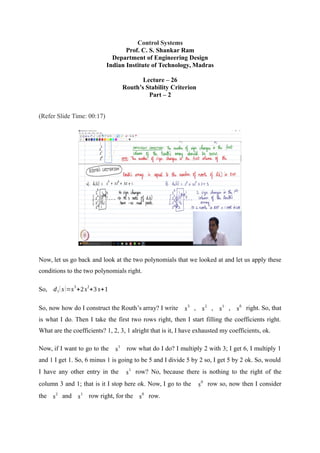
1. Control Systems
Prof. C. S. Shankar Ram
Department of Engineering Design
Indian Institute of Technology, Madras
Lecture – 26
Routh’s Stability Criterion
Part – 2
(Refer Slide Time: 00:17)
Now, let us go back and look at the two polynomials that we looked at and let us apply these
conditions to the two polynomials right.
So, d1(s)=s
3
+2s
2
+3 s+1
So, now how do I construct the Routh’s array? I write s
3
, s
2
, s
1
, s
0
right. So, that
is what I do. Then I take the first two rows right, then I start filling the coefficients right.
What are the coefficients? 1, 2, 3, 1 alright that is it, I have exhausted my coefficients, ok.
Now, if I want to go to the s
1
row what do I do? I multiply 2 with 3; I get 6, I multiply 1
and 1 I get 1. So, 6 minus 1 is going to be 5 and I divide 5 by 2 so, I get 5 by 2 ok. So, would
I have any other entry in the s
1
row? No, because there is nothing to the right of the
column 3 and 1; that is it I stop here ok. Now, I go to the s
0
row so, now then I consider
the s
2
and s
1
row right, for the s
0
row.

2. So, what do I do? I do the same process; 5 by 2 times 1 minus 2 times, you know when you
do not have an entry you take it as 0 ok; that is once not the first entry, but then the other
entries right. When you have reached s
1
row you do not have any entry here right so, you
take it as a null entry. So, 5 by 2 times 1 minus 2 times 0 is 5 by 2 and then 5 by 2 you divide
by 5 by 2 itself, what will you get? You will get 1.
Rouths array:
s
3
1 3
s
2
2 1
s
1
5/2 -
s
0
1 -
So now, let us look at the first column of the Routh’s array right. What can you observe?
Student: No sign changes.
No sign changes right because you one can observe that all entries are positive. So, this
implies that all 3 roots of d1(s) have negative real parts. So, I hope it is clear how we
applied it here right. So, please note you know I am not calculating the exact roots per se
right. Did I ask you to solve the polynomial for the roots? No, right that is what I am
reiterating here right, at this stage we are only interested in figuring out the location of the
roots ok. So, we did not solve for the roots. So, I am we are only concluding that all 3 roots
are in the left half complex plane, where we need we need to solve the equation right to get
the exact values of the roots ok.
So, that is that is the first polynomial. So, now, let us go to the second polynomial. So, what
happened in d2(s) ?
d2(s)=s
3
+2s
2
+s+3
So, let us do the Routh’s array construction once again s
3
,s
2
,s
1
,s
0
right. So, we have once
again we fill in the first two rows 1 2 1 and 3 right.

3. Now, we want to calculate for the s
1
row. What do we do? We multiply 2 with 1 subtract 1
and 3. What are we going to get?
Student: [Inaudible]
-1 right, -1 I divide by 2 I will get -1 by 2 and that is it right I I have exhausted my
coefficients. So, we come to the s
0
row, for the s power 0 row we consider these two rows
right. So, minus 1 by 2 times 3 is going to be minus 3 by 2, minus 3 by 2 minus of 2 times
null entry is going to be just minus 3 by 2 and minus 2 by 2 divided by minus 1 by 2 is going
to be.
Student: 3.
3. So, we immediately look at the first column of the Routh’s array. What can we see?
Rouths array:
s
3
1 1
s
2
2 3
s
1
-1/2 -
s
0
3 -
Student: 2 sign changes.
There are 2 sign changes. How come there are 2 sign changes? You see that from 2 to -1 by 2
is 1 sign change, from -1 by 2 to 3 here is another sign change ok. So, that is how we get 2
sign changes here ok. What does it imply?
Student: [Inaudible]
So, this implies that there are 2 roots in RHP and obviously, where should the third root be?
In LHP right so, plus 1 root in LHP ok. Yes please.

4. Student: [Inaudible]
No, why not? That is a good point ok. How come in this example, we are sure that it is not in
the on the jω axis ok. So, let us argue from two perspectives ok. So, that is a good
question, let me repeat this question. So, if you if you logically apply whatever we have
learnt till now, you know like the only conclusion we can draw based on the facts that we
have written under the Routh’s criteria is that there are 2 sign changes. So, 2 roots should be
in the right of plane. So, this is a third order polynomial right so, totally there are going to be
3 roots. So, 2 roots are in the right of complex plane so, we are left with only 1 root ok.
Where does the 1 remaining root lie? Obviously, there are two ways to eliminate the jω
axis; first is by looking in the Routh’s array you see that there are no 0 entries ok. So, as I told
you tomorrow we look at special cases you know that rules out the jω axis. Second thing
you can look at the polynomial itself, see this is a third order polynomial right you have 1
remaining root. So, if I want the 1 remaining root to be on the jω axis right, I can have
two possibilities. Either it should be the origin or it should be a complex conjugate pair on the
jω axis right. Complex conjugate pair is ruled out, why?
Student: Because only 1.
Because I have only 1 remaining root, complex conjugate pair means I need 2 more
remaining roots right that is gone and so, the only possibility which is left is at the origin. If
you have a root of a polynomial at the origin the constant term must be 0. Is the constant term
0 here? No alright. So, that is the second line of argument so, we are ruling out j omega axis.
Student: Because we got 2 roots, we got 1 root [Inaudible]
You may have, but once again that is a good point. Let us say we have an example, there is
only 1 sign change right, let us say a third order polynomial we have only 1 sign change.
Question is I am left with 2 remaining roots, I can still have let us say a complex conjugate
pair on the jω axis; possible. But still in that example if you in your first column of the
Routh’s array, if you do not have a 0 that you are you rule out that possibility ok. As I told
you we are going to do that tomorrow right. So, yeah I think that is a good question ok, I
hope you do not follow that result right yeah ok.

5. (Refer Slide Time: 08:26)
So, let me write down the general Routh’s stability criteria then we will go back to our
example that we are doing it last class and complete it ok. So, let me write down the Routh’s
stability criteria ok. So, you see that whatever we have been discussing till now applies to any
polynomial right; you can encode polynomials in any application. Now, we are going to apply
it to control theory ok.
So, I hope you can see how mathematics is applied to our subject of discussion right, which is
control design right. So, we will now see how we are going to apply it to our thing.
Routh’s Stability Criteria:
Consider a system whose transfer function is
n(s)
d(s)
. This system would be BIBO stable
(asymptotically stable) iff:
a) All coefficients of d(s) are non zero and of the same sign.
b) The first column of the Rouths array constructed using the coefficients of d(s) has all
entries being non-zero and of the same sign.
So, once again please note that BIBO stability means you know like you cannot have poles
on the imaginary axis also right, that is ruled out. So, I cannot say I will have a 0 on the first
column; no I should have non-zero entries in the first column and they should all be of the

6. same sign ok. So, those are the two conditions as far as the Routh’s stability criteria is
concerned ok. This is what is called as Routh’s stability criteria. So, we will go back and now
apply this Routh’s stability criteria to the problem that we were doing ok.
We are doing this problem right, where we were looking at the PI controller and we figured
out that the closed loop characteristic equation is s
3
+(K p+1)s+Ki=0 right.
(Refer Slide Time: 13:00)
So, now, the roots of this polynomial will be the closed loop poles. So, do you think the PI
controller will stabilize this closed loop system? No why not?
I do not even need to go any further right, why not the necessary condition is not satisfied
right. the coefficient of s2
is zero right. So, this implies that there are no values of Kp and Ki
can stabilize the closed loop system that is the implication of this result correct. So, the PI
controller will not work. So, now, you see why we digressed and learn the Routh’s stability
criteria and came here right.
So, you can see that our analysis becomes more simple right. So, now, as the next step let us
try the PD controller because, for this system let us go ahead and try the PD controller ok. So,
PD controller means its transfer function is Kp + Kd s. So, we follow the same framework ok.
G(s)=C(s) P(s)=
Kd s+Kp
s
2
+1

7. (Refer Slide Time: 15:03)
C.L.T.F =
G(s)
1+G (s) H (s)
=
Kd s+K p
s
2
+1
1+
K d s+Kp
s
2
+1
=
Kd s+K p
s
2
+Kd s+(K p+1)
So, immediately we see that this is a polynomial of order 2 right; the closed loop system with
a derivative PD controller is still the second order system ok. With this you know, like
immediately we see that as I discussed for polynomial still order 2 the necessary and
sufficient condition is all coefficients must be non-zero and of the same sign ok. So, this
implies that the closed loop system would be BIBO stable if and only if the all the
coefficients must be non-zero and the same sign right; s
2
term the coefficient is plus 1. So,
already 1 coefficient is positive. So, we must have Kd > 0, Kp + 1 > 0. So, this implies that Kd
> 0 and Kp > -1 is the feasible region for stability.
So, if I want to plot this in the controller parameter space, we have Kp on the horizontal axis,
let us say Kd on the in the vertical axis right. So, how will I plot Kd > 0? Kd greater than 0 is
this half plane right, isn’t it right. How do I plot Kp > - 1? First I draw Kp equals minus 1 and
any region to the right of it is going to be Kp greater than minus 1 right. So, consequently the
feasible region is going to be the intersection of the two regions right correct; this is the
feasible region. Alright this is what I called as a controller parameter space right.

8. If I say calculate the feasible region in the controller parameter space, this is what you need to
do for the controller design, fine. So, as a very simple exercise for you to do, consider the
general second order polynomial a0 s
2
+a1 s+a2 . Apply the Routh’s array to that and
convince yourself that the necessary condition is also sufficient ok. You will see that the first
column will have a0 a1 and a2 ok. So, what was necessary will also become sufficient for
polynomial still order 2 ok. So, that is the, what to say, criteria for the for orders polynomial
still order 2 ok. So, is it clear? Yeah.