SlideShare a Scribd company logo
1 of 24
Download to read offline
Elementary Numerical Analysis
Prof. Rekha P. Kulkarni
Department of Mathematics
Indian Institute of Technology, Bombay
Lecture No. # 24
Tutorial -3
Today, we are going to solve some problems. So, first we are going to show that product
of two lower triangular matrices is lower triangular, if the diagonal entries of both the
lower triangular matrices, if they are equal to 1, then the product also has diagonal
entries is equal to 1.
Then, we will show that inverse of a lower triangular matrix is again lower triangular;
and then we had used these results to show uniqueness of the LU decomposition. So, I
will recall that result.
(Refer Slide Time: 01:06)
So, here is the first tutorial problem, that you have got two matrices L and M, say of size
n by n, and they are unit lower triangular; that means, the diagonal entries, they are equal
to 1. So, we want to show that L into M is also a unit lower triangular matrix. So, the
proof is going to be straight forward, we will just look at the multiplication of these two
matrices.
(Refer Slide Time: 01:36)
The structure of our matrix L is going to be of this form. Along the diagonal, we have
got 1, the part which lies below the diagonal it can have non-zero entries or zero entries.
But definitely, the elements which are above the diagonal they are going to be 0. So, that
means, l ij is equal to 0, if i is less then j, i denotes the row index and j denotes the
column index. And l ii is equal to 1 i is equal to 1 2 up to n. Matrix M is going to have
similar form and now we look at the product of L into M.
(Refer Slide Time: 02:22)
So, we have l ij is equal to 0 m ij is equal to 0, if i less then j and l ii is equal to m ii is
equal to 1 for i going from 1 2 up to n ijth element of matrix LM. We denote by LM in
the bracket i,j. By definition of matrix multiplication, this will be given by summation l
ik m kj k goes from 1 to n. So, it is ith row of L multiplied by jth column of m.
Now, using the fact that l ij is equal to 0, if i less then j, you are going to have summation
k goes from 1 to i, because when k is equal to i plus 1 l ii plus 1 will be 0. So, this is
going to be summation k goes from 1 to i l ik m kj. We are interested in the elements of l
m, when i is less than j. So, for that case i less than j m kj will be 0 for k going from 1 2
up to i, because for k is equal to 1 2 up to i j will be bigger than k. And m has the
property that m ij is 0, if i less than j. And hence this summation… in this summation m
kj’s they are going to be 0. So, you get LM i, j is equal to 0. So, as in the case of L and M
when you consider the elements LM ij when i less then j they are equal to 0.
So, now it remains to show that the diagonal entries they are equal to 1. So, now, we will
look at diagonal entry of LM say LM i, i that will be given by ith row of l multiplied by
ith column of m.
(Refer Slide Time: 04:38)
And then we obtain LM i, i to be summation k goes from 1 to n l ik m ki. Now, as before
this summation reduces to summation k goes from 1 to i l ik m ki. The only non-zero
term in the summation is going to be when k is equal to i. So, you get this to be equal to l
ii m ii and this is equal to 1. So, thus product of two lower triangular matrices is going to
be a lower triangular matrix and if the diagonal entries of both the matrices they are
equal to 1, then the product also has similar property.
Now, the next example, which we want to consider is if L is a lower triangular matrix,
then its inverse is going to be again a lower triangular. So, you start with a invertible
lower triangular matrix and we want to show that its inverse is lower triangular; when we
had discussed Gauss elimination method, we had said that finding a inverse using the
classical formula is something not advisable, because it is very expensive. So, what one
should do is, if one wants to find the inverse of a matrix, then you solve the system Ax is
equal to b for right hand side b is equal to e 1, e 2, e n, which are the canonical vectors.
And then, when you consider l x is equal to e j, whatever result you get you should write
it as a jth column. So, that gives you inverse of A, it is this result we are going to use to
show that inverse of a lower triangular matrix is lower triangular
(Refer Slide Time: 06:49)
The computation of A inverse: A inverse is given by A inverse e 1, A inverse e 2, A
inverse e j, A inverse e n . So, the jth column of A inverse is C j, which is equal to A
inverse e j equivalently, you get a C j is equal to e jj going from 1 2 up to n. So, thus the
column the jth column of A inverse is obtained by solving system of linear equations A
C j is equal to e j, where e j is the canonical vector with 1 at jth place and 0 else where.
(Refer Slide Time: 07:36)
Look at L to be a unit lower triangular matrix, because it is unit lower triangular,
determinant of L will be equal to 1. The product of the diagonal entries and hence it will
be invertible. Now, we want to show that L inverse is also unit lower triangular. So, you
write L inverse as its columns L inverse e 1 L inverse e 2 L inverse e n the jth column C j
of L inverse is given by C j is equal to a 1j a 2j a nj, which is equal to L inverse e j. So,
that gives you L of c j is equal to e j a, system of equation to solve.
(Refer Slide Time: 08:24)
Now, our matrix L it has got 1 along the diagonal entries 0 above the diagonal and below
diagonal, it is given by this multiplied by say jth column I am denoting the jth column by
b 1j b 2j b nj is equal to right hand side, which is ej; So, 1 at jth place and 0 elsewhere.
Since the matrix L is lower triangular, we can use forward substitution. So, the first
equation has only 1 unknown , but its b 1j and equating you get b 1 j to be 0. Now,
second equation will be l 21 b 1j plus b 2j is equal to 0. Now, b 1j is already 0. So, you
get the b 2j is equal to 0 and continuing in this fashion, you get b j minus 1 j is equal to 0
when you look at jth equation, the jth equation will be l j1 b 1j l j2 b 2j l jj b jj.
Where l jj is going to be 1 and since b 1 j b 2 j b j minus 1 j is equal to 0, you obtain b jj
to be equal to 1, if you look at j plus first equation it will have l j plus 1 j b jj plus bj plus
1 j is equal to 0. Now, b jj is equal to 1. So, you are going to get b j plus 1 j is equal to
minus l j plus 1 j. So, that is how you can calculate the jth column and in the j th column.
The important thing is you get first j minus one entries to be 0, the jth entry to be equal to
1and then remaining entries they may be non-zero or they may be 0.
It depends on your matrix l, but definitely in the jth column first j minus 1 entries they
are going to be equal to 0 and jth entry is going to be equal to 1. So, that is what will
make our inverse to be unit lower triangular.
(Refer Slide Time: 10:51)
So, when you look at L inverse it is going to have, 1 along the diagonal - star means
either it is zero or it is non-zero and above you are getting all 0. So, we get L inverse also
to be unit lower triangular. Now, when you look at upper triangular matrices, then
whether product of two upper triangular matrices is upper triangular whether inverse of
upper triangular matrix is upper triangular. So, the result is true and we can deduce this
result for upper triangular matrices by taking the transpose, like we have proved that
product of two lower triangular matrices is again a lower triangular. Now, if you are
looking at two upper triangular matrices say U 1 and U 2, then when you take transpose,
transpose of upper triangular matrix will become lower triangular matrix. So, take the
transpose then use the fact that product of two lower triangular matrices is again a lower
triangular matrices and then again take the transpose, same idea for showing that inverse
of upper triangular matrix is upper triangular.
And there we use the fact that the inverse and transpose, these two operations they
commute in the sense that a inverse transpose is going to be same as a transpose inverse,
whether I take inverse first and then take transpose or take transpose and then take
inverse the result is going to be the same.
(Refer Slide Time: 12:46)
So, let us show this; now, for upper triangular matrices U and V are unit upper triangular
take the transpose, then they become unit lower triangular. What we have proved just
now is V transpose U transpose that is going to be a unit lower triangular matrix, but V
transpose U transpose is nothing but transpose of U into V. So, if U into V transpose is
unit lower triangular UV is going to be unit upper triangular.
So, U and V unit upper triangular implies their product is also unit upper triangular. For
the inverse now, U is unit upper triangular take its transpose it becomes unit lower
triangular take its inverse that is going to be unit lower triangular, which we proved just
now because the operation of transpose and inverse commute, this will be U inverse
transpose. Now, if U inverse transpose is unit lower triangular, then U inverse has to be
unit upper triangular.
(Refer Slide Time: 13:57)
And now using these two results, let us recall the result of uniqueness of LU
decomposition. So, if you have A is equal to L 1 U1 is equal to L 2 U 2. Where L 1 and
L 2 are unit lower triangular matrices U 1, U 2 are upper triangular matrices and
invertible, then from this relation I can deduce that L 2 inverse L 1 is going to be equal to
U 2 U 1 inverse I pre-multiply by L 2 inverse and post multiply by U 1 inverse now left
hand side is a unit lower triangular matrix right hand side is a upper triangular matrix, if
both are equal then both of them they should be diagonal matrix and then because the
diagonal entries of L 2 inverse L 1 they are going to be 1, the diagonal matrix is nothing
but the identity matrix.
So, this is the uniqueness of LU decomposition. So, if a is invertible then A can be
written uniquely as L into U, when we proved LU decomposition of the matrix A we had
made an additional assumption that look at the principle leadings sub matrix that is
formed by first k rows and first k columns of our matrix. So, you take a square matrix, if
its determinant is not equal to 0 for k is equal to 1 2 up to n.
Then we proved that under this assumption a can be written uniquely as L into U. Now,
we want to prove the converse that suppose, A is a invertible matrix and it is given to us
that it can be written as L into U. Where L is unit lower triangular, U is upper triangular
then we want to show that determinant of a k is not equal to 0. So, thus what we are
going to show is if A is invertible you can write a as equal to L into U, if and only if
determinant of A k is not equal to 0 for k is equal to 1 2 up to n. Now, in order to prove
this result, portioning of this matrix it helps. Let us do one thing, we have got our n by n
matrix and we are already considering the leading principles of matrix. So, you have got
sub matrix which is formed by first k rows and first k columns. So, look at our remaining
sub matrices.
(Refer Slide Time: 16:58)
So, A is A 11 A 12, A 21 A 22, where A 11 is k by k matrix. So, this A 11 we have been
calling it A k; A 12 will be formed by first k rows and next n minus k columns last n
minus k columns. So, the size of A 12 is k into k by n minus k matrix A 21 that is formed
by n minus k rows and k columns. So, it will be n minus k by k and A 22 will be matrix
of size n minus k by n minus k.
(Refer Slide Time: 17:44)
Next, we look at multiplication of two n by n matrices A and B. So, C is equal to AB
then, if you partition matrices AB and C in a similar manner. Then we are going to have
C 11 is equal to A 11 B1 plus A 12 B 21, the result is also going to be true for C 12 like
C 12 will be given by first row into second column.
So, C 12 will be A 11 B 12 plus A 12 B 22 and so, similarly, for C 21 and C 22. So, it is
as if we are treating this as 2 by 2 matrix, but for our result we need only the result about
C 11. So, let us prove this result. Now, before we proceed notice that C 11is going to be
k by k matrix A 11 is k by k B 11 is k by k. So, this is going to be k by k. A 12 is k by n
minus k B 21 is n minus k by k. So, when you take their product you again get a k by k
matrix. So, in order to prove this result we use the usual formula for matrix
multiplication.
(Refer Slide Time: 19:28)
So, C ij will be given by ith row of a into jth column of b. So, it is summation p goes
from 1 to n a ip b p j. This sum I split into two sums p going from 1 to k and p going
from k plus 1 to n now you look at. So, our i and j they are going to be lie between one
and k. So, 1 less than or equal to i j less than or equal to k then look at a ip. So, i is
between 1 and k p is between 1 and k. So, a ip will be nothing but i pth element of A 11
then b pj p is between 1 and k j is between 1 and k. So, b p j will be nothing but B 11 p j
plus. Here i is between 1 and k, but p is between k plus 1 to n p means the column.
So, that is why this a i p will be i pth element of A 12. So, it is A 12 i p and then b p j.
So, b pj will be nothing but p is between k plus 1 to n j is between 1 and k. So, that is B
21 p j. So, this proves C 11 is equal to A 11 B 11 plus A 12 B 21. Now, let us use this
fact for lower triangular matrices.
(Refer Slide Time: 21:26)
So, suppose a is a invertible matrix which is given to us that it can be written as L into U.
Let A k denote the principle leadings sub matrix of order k and our claim is that
determinant of A k is not equal to 0 for k is equal to 1 2 up to n.
(Refer Slide Time: 21:50)
So, this is given to us that A is equal to L into U L being a lower triangular matrix with
diagonal entries is equal to one determinant of L will be equal to 1. So, determinant of U
is equal to determinant of A, which is not equal to 0, because A is given to be invertible
matrix. U being an upper triangular matrix determinant of U will be product of the
diagonal entries u 11 u 22 u nn and this not equal to 0 implies u ii to be not equal to 0.
Now, partition matrix A l and U as before. Because L is lower triangular L 12 is going to
be a zero matrix, because U is upper triangular matrix U 21 is going to be a zero matrix.
Now, A 11 will be given by L 11 into U 11, because the other L 12 U 21 term both of
them they are 0. So, in our notation A k is going to be equal to L k into U k. So,
determinant of A k is equal to determinant of U k, because again the diagonal entries of
L k is equal to 1 determinant U k is U 11 U 22 U kk which is not equal to 0.
(Refer Slide Time: 23:22)
And thus we have proved that if A is an invertible matrix, this invertible is important,
which can be written as L into U. Then the determinant of the principle leading sub
matrix of order k is going to be non-zero for k is equal to 1 2 up to n.
(Refer Slide Time: 23:42)
Now, as a simple example, let us calculate LU decomposition of this matrix. Now, at this
stage I will like to recall that in order to find LU decomposition, what you can do is
consider matrix A use Gauss elimination method to reduce it to upper triangular matrix.
So, that is going to give you matrix U. And the matrix L will be unit lower triangular -
constructed using the multipliers used in the Gauss elimination method. So, we are
considering Gauss elimination without partial pivoting when we use gauss elimination
with partial pivoting, we get LU decomposition of A.
If you are using Gauss elimination with partial pivoting, which involves interchange of
rows then LU decomposition is not of the matrix A, but it is the matrix P into A; where P
is the permutation matrix obtained by finite number of row interchanges in the identity
matrix. So, let us reduce this 3 by 3 matrix to upper triangular form and then find L and
U? One can also find directly L and U by multiplying L and U and equating the
corresponding entries. But the way I am proving is using Gauss elimination method.
(Refer Slide Time: 25:28)
So, I want to reduce this to upper triangular form. So, first I want to introduce 0s in the
first column, below the diagonal. So, I do second row minus 2 times R 1 and third row
minus 3 times R 1. So, our multipliers are 2 and 3. So, they are going to appear in the
first column of l. So, the first column of l will consist of 1 here and then these multipliers
2 and 3 when I do these operations these two are 0, then 2 into 2 is 4. So, 5 minus 4 you
will get 1 2 into 3 is 6. So, that gives you this entry to be 2 then 8 minus 3 into 2 that will
give you 2 and then 14 minus 3 into 3 that will give you 5.
So, this is the first stage of Gauss elimination method in the second step you look at the
second column and try to make this entry to be 0. So, this can be achieved by R 3 minus
2 times R 2 multiply second row by 2 and subtract from the third row. So, you will get 0
here 2 into 2 is 4; 5 minus 4 this will be 1. Now, the multiplier is 2. So, that is going to
occupy this place. So, you will get U to be matrix upper triangular given by here and L to
be lower triangular, which is given by this.
(Refer Slide Time: 27:03)
So, now I want to consider some properties of positive definite matrices; for the positive
definite matrix the definition is: it should be a symmetric matrix and x transpose A x
should be bigger than 0 for every non-zero vector, now this second property something
difficult to verify. For all non-zero vectors we want x transpose A x to be bigger than 0.
(Refer Slide Time: 27:42)
So, now, we are going to prove a necessary condition that if matrix A is positive definite
then its diagonal entries they have to be strictly bigger than 0. So, if you are given a
matrix A with one of the diagonal entry to be either a negative real number or 0 then
such a matrix cannot be positive definite.
Now, for special case of diagonal matrices we are going to show that d is positive
definite, if and only if diagonal entries they are bigger than 0 for general matrices it is a
necessary condition it is not sufficient that it can happen that diagonal entries are all
bigger than 0, but still matrix is not positive definite. But for the diagonal entries they are
for the diagonal matrices, it is a necessary and sufficient condition that the entries d ii
should be bigger than 0 and proof of both these results they are simple, we are going to
use a fact that ei and ej are canonical vectors. So, if I look at e j transpose A e ii get i jth
entry of my matrix A.
(Refer Slide Time: 29:27)
So, the diagonal entries they will be given by e i transpose A e i a is positive definite. So,
you look at e i transpose A e i. e i transpose is row vector with one at ith place, A ei is
going to be ith column of A. So, it is a 1i a 2i a n i, when i take the multiplications, I get
a ii since e i is a non-zero vector and a is positive definite e i transpose a ei is bigger than
0 and hence we get the diagonal entries of a to be bigger than 0. Now, let us look at
diagonal matrix.
(Refer Slide Time: 30:09)
So, suppose D is diagonal matrix with diagonal entries to be d1, d2, d n, we are going to
show that this is positive definite if and only if d i is bigger than 0. Now, this way
implication that d positive definite implies d i is bigger than 0, this we just now proved
for any general matrix. So, it is going to be true for diagonal matrix also. Now, let us
look at the converse. So, this is given to us that D is a diagonal matrix d i's are bigger
than 0. So, the first thing is d transpose is equal to D and now let us look at x transpose D
x, you have got D to be diagonal matrix. So, x transpose D x will be nothing, but
summation j goes from 1 to n d j x j square x is a non-zero vector.
That means, at least one of the entry is non-zero which will make this sum to be bigger
than 0 and that makes diagonal matrix D to be positive definite. I want to consider again
Gauss elimination method. So, in the Gauss elimination method, we have proved LU
decomposition for example, for positive definite matrices or for diagonally dominant
matrices. So, you have got a matrix A, you do the first step of Gauss elimination method
and then in the next step you are going to work only on the n minus 1 by n minus 1 sub
matrix. So, I start with matrix A to be positive definite, now the next sub matrix, which I
am going to work on or after first step of gauss elimination method, whether this
property whether it will be preserved.
Now, the answer to that is yes, but I am going to prove only the property that if your
matrix A is a symmetric matrix, you do first type of the Gauss elimination method and
the sub matrix which you are going to work in the next step, it retains the symmetric
property. So, it is a important property, because it can help us to reduce our computations
by half.
(Refer Slide Time: 32:51)
So, here is the first type of Gauss elimination method. This is a matrix A and we want to
introduce 0s in the first column below the diagonal. So, our multipliers are going to be m
i1 is equal to a i1 by a 11and then the operations which we perform are R i becomes R i
minus m i1 R 1 multiply the first row R 1 by m i1 and subtract from ith row. When we
do this, this is the matrix which we obtain. So, suppose a is symmetric then whether this
n minus 1 by n minus 1 sub matrix, which is formed by second, third and nth row and
second, third and nth column. So, this matrix is also going to be symmetric this is what
we want to show.
Now, the modified entries here they are given by a i j modified entry one is equal to a i j
minus m i1 a 1j, because this is our operation we are subtracting the first row from the ith
row. So, this is what we are doing a ij minus m i one a 1j, a ij will be a entry in the ith
row, we consider the corresponding entry in the first row. So, that will be a 1j and
multiply by m i1 and subtract.
(Refer Slide Time: 34:38)
So, our matrix A it becomes a 11 R 1 tilde 0 matrix and A 1, where A 1 is the n minus 1
by m minus 1 sub matrix.
(Refer Slide Time: 34:55)
This is our question, if A is symmetric then whether A 1 is also symmetric. So, we look
at a ij 1 by definitions it is a ij minus m i1 a 1j, what was m i1, it was a i1 by a11. So, I
substitute now, I use the fact that A is symmetric; that means, a ij is equal to a ji. So, you
get a ji minus a i1 will be same as a 1i, which I am writing here a 1j will be same as a j1,
which I am writing here and then a 11.
So, you get a ji minus a j1 by a 11 will be nothing but m j1 and then a 1i. Now, this will
be nothing but a ji 1. So, thus if your matrix A is symmetric then a1 is also going to be a
symmetric matrix. Now, it is also true that if a is positive definite, then a 1 is positive
definite if A is diagonally dominant matrix, then A 1 will also be diagonally dominant.
So, the matrix is diagonally dominant will mean that we do not have to do row
interchanges then then the matrix is positive definite then. In fact, we have seen that we
can write its Cholesky decomposition. So, again no row interchanges, we had introduced
row interchanges for the sake of stability, when we looked at backward error analysis,
we saw that we should not divide by a small number.
So, you have to like that is why one considers or it is important that if you do not have to
do row interchanges then it is it saves our computational efforts. Now, these two results
they are a bit involved. So, I am not going to prove those results, but we are going to
consider the effect on the solution if you multiply column of the coefficient matrix by a
non-zero number.
Look at the system of equations a x is equal to b, in this if I look at a say ith equation and
multiply throughout by a non-zero number, then I am not changing the system my
solution is going to remain the same. On the other hand, if I multiply column of
coefficient matrix by a non-zero number then my solution will be different my system is
different, now what we are going to show is that if you multiply jth column of the matrix
A by say a number alpha whereas, phi is not equal to 0.
The only change in the solution is going to be in the jth component and that jth
component gets multiplied by one by alpha our matrix is invertible matrix. If I multiply a
column by a non-zero number alpha determinant of the new matrix will get multiplied by
alpha. So, if a is invertible my new matrix also will be invertible, because the
determinant will be not equal to 0 in doing this, I am changing my system. So, I get a
new solution. So, when you compare the new solution with the original solution the only
difference will be in the jth component all other components of the original solution and
a new solution they are going to be the same.
The jth component effect will be what was earlier x j that will become one upon alpha
times x j. So, when we consider later on about the scaling of the matrix in order to make
it well conditioned, this result is going to be important. Now, the proof of this result is
straight forward. What we are going to do is a x is equal to b. So, write xx is our column
vector x1,x2, xn this x we can write as x 1 e 1 plus x 2 e 2 plus x n en where e j's are the
canonical vector apply a and then see what you get.
(Refer Slide Time: 40:49)
So, we have a non-singular system; that means, the coefficient matrix A is invertible it is
altered by multiplication of its jth column by alpha not equal to 0, then the solution is
altered only in the jth component, which is multiplied by 1 by alpha.
(Refer Slide Time: 41:13)
So, we have got A x is equal to b x is column vector x1, x2, xn this will be equal to x
1e1plus x 2e2 plus xn en. So, when you consider, when you apply A, then Ax will be x1
A e1 plus x2 A e2plus x n A en is equal to b A ej is the jth column, we are going to
multiply the jth column by alpha. So, the new system is a tilde which is equal to Ae1 A
ej minus 1, these columns they remains as before the jth column becomes alpha times A
e j and the j plus first column onwards up to th column they all remain the same. So,
now, I can from this relation I can write this as x j by alpha and alpha times A e j. So, I
am multiply and divide by alpha. So, I am going to have this is same as equal to b,
because in this I am just multiplying and dividing by alpha.
So, I will get now this is nothing, but A tilde x tilde is equal to b and what will be x tilde
it will be x1 x2 x j minus 1 the jth 1 will be x j by alpha and the last 1 is going to be x n.
So, we had original system Ax is equal to b and when you alter it then x tilde which is
the new solution it gets altered by only dividing x j by alpha. So, these were some of the
problems, which are based on our Gauss elimination method and also on the LU
decomposition and in the next tutorial it will be based on norm of a matrix. So, for the
gauss elimination method when we want to see the effect of of the perturbation then we
need to talk about the norms and the norms come into picture.
So, here where some of the problems now about the LU decomposition what you can do
is you can try to find LU decomposition directly, you should get the same result and one
of the important result which we proved in today’s tutorial is a invertible matrix has LU
decomposition if and only if determinant of A k is not equal to 0, where A k is the
leading sub matrix, leading principle sub matrix. We had similar result for positive
definite matrix; that means, it was the if and only if, result that a is positive definite if
and only if you can write a as mm transpose, where M is going to be an invertible matrix.
So, thank you.

More Related Content

What's hot

Inside maths : 1 Jaydeep Shah
Inside  maths : 1 Jaydeep ShahInside  maths : 1 Jaydeep Shah
Inside maths : 1 Jaydeep ShahJAYDEEP SHAH
 
How Unstable is an Unstable System
How Unstable is an Unstable SystemHow Unstable is an Unstable System
How Unstable is an Unstable Systemidescitation
 
Mba Ebooks ! Edhole
Mba Ebooks ! EdholeMba Ebooks ! Edhole
Mba Ebooks ! EdholeEdhole.com
 
Intervals of validity
Intervals of validityIntervals of validity
Intervals of validityTarun Gehlot
 
Oscillation of Solutions to Neutral Delay and Advanced Difference Equations w...
Oscillation of Solutions to Neutral Delay and Advanced Difference Equations w...Oscillation of Solutions to Neutral Delay and Advanced Difference Equations w...
Oscillation of Solutions to Neutral Delay and Advanced Difference Equations w...inventionjournals
 
Review power series
Review power seriesReview power series
Review power seriesTarun Gehlot
 
Oscillation of Solutions to Neutral Delay and Advanced Difference Equations w...
Oscillation of Solutions to Neutral Delay and Advanced Difference Equations w...Oscillation of Solutions to Neutral Delay and Advanced Difference Equations w...
Oscillation of Solutions to Neutral Delay and Advanced Difference Equations w...inventionjournals
 
Modelling with first order differential equations
Modelling with first order differential equationsModelling with first order differential equations
Modelling with first order differential equationsTarun Gehlot
 
Applications of differential equations by shahzad
Applications of differential equations by shahzadApplications of differential equations by shahzad
Applications of differential equations by shahzadbiotech energy pvt limited
 
AP Calculus - Mini Exam Review
AP Calculus - Mini Exam ReviewAP Calculus - Mini Exam Review
AP Calculus - Mini Exam Reviewk_ina
 

What's hot (20)

Lec45
Lec45Lec45
Lec45
 
Inside maths : 1 Jaydeep Shah
Inside  maths : 1 Jaydeep ShahInside  maths : 1 Jaydeep Shah
Inside maths : 1 Jaydeep Shah
 
Lec57
Lec57Lec57
Lec57
 
Lec26
Lec26Lec26
Lec26
 
Lec10
Lec10Lec10
Lec10
 
Lec55
Lec55Lec55
Lec55
 
Lec11
Lec11Lec11
Lec11
 
Lec37
Lec37Lec37
Lec37
 
How Unstable is an Unstable System
How Unstable is an Unstable SystemHow Unstable is an Unstable System
How Unstable is an Unstable System
 
Lec46
Lec46Lec46
Lec46
 
Mba Ebooks ! Edhole
Mba Ebooks ! EdholeMba Ebooks ! Edhole
Mba Ebooks ! Edhole
 
Intervals of validity
Intervals of validityIntervals of validity
Intervals of validity
 
Oscillation of Solutions to Neutral Delay and Advanced Difference Equations w...
Oscillation of Solutions to Neutral Delay and Advanced Difference Equations w...Oscillation of Solutions to Neutral Delay and Advanced Difference Equations w...
Oscillation of Solutions to Neutral Delay and Advanced Difference Equations w...
 
Review power series
Review power seriesReview power series
Review power series
 
Oscillation of Solutions to Neutral Delay and Advanced Difference Equations w...
Oscillation of Solutions to Neutral Delay and Advanced Difference Equations w...Oscillation of Solutions to Neutral Delay and Advanced Difference Equations w...
Oscillation of Solutions to Neutral Delay and Advanced Difference Equations w...
 
Modelling with first order differential equations
Modelling with first order differential equationsModelling with first order differential equations
Modelling with first order differential equations
 
Lec6
Lec6Lec6
Lec6
 
Transform idea
Transform ideaTransform idea
Transform idea
 
Applications of differential equations by shahzad
Applications of differential equations by shahzadApplications of differential equations by shahzad
Applications of differential equations by shahzad
 
AP Calculus - Mini Exam Review
AP Calculus - Mini Exam ReviewAP Calculus - Mini Exam Review
AP Calculus - Mini Exam Review
 

Viewers also liked

Viewers also liked (20)

Lu decomposition
Lu decompositionLu decomposition
Lu decomposition
 
Gauss jordan and Guass elimination method
Gauss jordan and Guass elimination methodGauss jordan and Guass elimination method
Gauss jordan and Guass elimination method
 
Es272 ch4b
Es272 ch4bEs272 ch4b
Es272 ch4b
 
Gauss Jordan
Gauss JordanGauss Jordan
Gauss Jordan
 
Digital design chap 3
Digital design   chap 3Digital design   chap 3
Digital design chap 3
 
LU Decomposition Fula
LU Decomposition FulaLU Decomposition Fula
LU Decomposition Fula
 
Métodos directos para la solución de sistemas de ecuaciones lineales
Métodos directos para la solución de sistemas de ecuaciones linealesMétodos directos para la solución de sistemas de ecuaciones lineales
Métodos directos para la solución de sistemas de ecuaciones lineales
 
Lenier Equation
Lenier EquationLenier Equation
Lenier Equation
 
IS 151 Lecture 8
IS 151 Lecture 8IS 151 Lecture 8
IS 151 Lecture 8
 
Unit5
Unit5Unit5
Unit5
 
Lu decomposition
Lu decompositionLu decomposition
Lu decomposition
 
M6800
M6800M6800
M6800
 
Ch5 epfm
Ch5 epfmCh5 epfm
Ch5 epfm
 
Gaussian elimination method & homogeneous linear equation
Gaussian elimination method & homogeneous linear equationGaussian elimination method & homogeneous linear equation
Gaussian elimination method & homogeneous linear equation
 
Gauss-Jordan Theory
Gauss-Jordan TheoryGauss-Jordan Theory
Gauss-Jordan Theory
 
Graphical Method
Graphical MethodGraphical Method
Graphical Method
 
Chp1 68000 microprocessor copy
Chp1 68000 microprocessor   copyChp1 68000 microprocessor   copy
Chp1 68000 microprocessor copy
 
Gaussian Elimination Method
Gaussian Elimination MethodGaussian Elimination Method
Gaussian Elimination Method
 
Gauss y gauss jordan
Gauss y gauss jordanGauss y gauss jordan
Gauss y gauss jordan
 
Solving linear programming model by simplex method
Solving linear programming model by simplex methodSolving linear programming model by simplex method
Solving linear programming model by simplex method
 

Similar to Lu decomposition

Stochastic Processes Homework Help
Stochastic Processes Homework HelpStochastic Processes Homework Help
Stochastic Processes Homework HelpExcel Homework Help
 
Free Ebooks Download ! Edhole
Free Ebooks Download ! EdholeFree Ebooks Download ! Edhole
Free Ebooks Download ! EdholeEdhole.com
 
pnp2.ppt
pnp2.pptpnp2.ppt
pnp2.pptham111
 
MC0082 –Theory of Computer Science
MC0082 –Theory of Computer ScienceMC0082 –Theory of Computer Science
MC0082 –Theory of Computer ScienceAravind NC
 
MTH391 Final Paper (1)
MTH391 Final Paper (1)MTH391 Final Paper (1)
MTH391 Final Paper (1)Kevin Johnson
 
Magnetic Monopoles, Duality and SUSY.pptx
Magnetic Monopoles, Duality and SUSY.pptxMagnetic Monopoles, Duality and SUSY.pptx
Magnetic Monopoles, Duality and SUSY.pptxHassaan Saleem
 
Introduction to the Theory of Computation, Winter 2003 A. Hevia and J. Mao S...
 Introduction to the Theory of Computation, Winter 2003 A. Hevia and J. Mao S... Introduction to the Theory of Computation, Winter 2003 A. Hevia and J. Mao S...
Introduction to the Theory of Computation, Winter 2003 A. Hevia and J. Mao S...parmeet834
 
Using Laplace Transforms to Solve Differential Equations
Using Laplace Transforms to Solve Differential EquationsUsing Laplace Transforms to Solve Differential Equations
Using Laplace Transforms to Solve Differential EquationsGeorge Stevens
 
Solving the boltzmann transport equation displaced using maxwell approximation
Solving the boltzmann transport equation displaced using maxwell approximationSolving the boltzmann transport equation displaced using maxwell approximation
Solving the boltzmann transport equation displaced using maxwell approximationalagumuthuakhilachoc
 
Series solutions airy's equation
Series solutions airy's equationSeries solutions airy's equation
Series solutions airy's equationTarun Gehlot
 

Similar to Lu decomposition (20)

Lec38
Lec38Lec38
Lec38
 
Lec54
Lec54Lec54
Lec54
 
Stochastic Processes Homework Help
Stochastic Processes Homework HelpStochastic Processes Homework Help
Stochastic Processes Homework Help
 
Lec6
Lec6Lec6
Lec6
 
Free Ebooks Download ! Edhole
Free Ebooks Download ! EdholeFree Ebooks Download ! Edhole
Free Ebooks Download ! Edhole
 
pnp2.ppt
pnp2.pptpnp2.ppt
pnp2.ppt
 
Lec14
Lec14Lec14
Lec14
 
Lec41
Lec41Lec41
Lec41
 
Stochastic Processes Homework Help
Stochastic Processes Homework HelpStochastic Processes Homework Help
Stochastic Processes Homework Help
 
Ch7 angular momentum
Ch7 angular momentumCh7 angular momentum
Ch7 angular momentum
 
MC0082 –Theory of Computer Science
MC0082 –Theory of Computer ScienceMC0082 –Theory of Computer Science
MC0082 –Theory of Computer Science
 
Lec60
Lec60Lec60
Lec60
 
MTH391 Final Paper (1)
MTH391 Final Paper (1)MTH391 Final Paper (1)
MTH391 Final Paper (1)
 
Magnetic Monopoles, Duality and SUSY.pptx
Magnetic Monopoles, Duality and SUSY.pptxMagnetic Monopoles, Duality and SUSY.pptx
Magnetic Monopoles, Duality and SUSY.pptx
 
Introduction to the Theory of Computation, Winter 2003 A. Hevia and J. Mao S...
 Introduction to the Theory of Computation, Winter 2003 A. Hevia and J. Mao S... Introduction to the Theory of Computation, Winter 2003 A. Hevia and J. Mao S...
Introduction to the Theory of Computation, Winter 2003 A. Hevia and J. Mao S...
 
Using Laplace Transforms to Solve Differential Equations
Using Laplace Transforms to Solve Differential EquationsUsing Laplace Transforms to Solve Differential Equations
Using Laplace Transforms to Solve Differential Equations
 
Lec42
Lec42Lec42
Lec42
 
Solving the boltzmann transport equation displaced using maxwell approximation
Solving the boltzmann transport equation displaced using maxwell approximationSolving the boltzmann transport equation displaced using maxwell approximation
Solving the boltzmann transport equation displaced using maxwell approximation
 
Series solutions airy's equation
Series solutions airy's equationSeries solutions airy's equation
Series solutions airy's equation
 
Vector and scalar
Vector and scalarVector and scalar
Vector and scalar
 

Recently uploaded

DeepFakes presentation : brief idea of DeepFakes
DeepFakes presentation : brief idea of DeepFakesDeepFakes presentation : brief idea of DeepFakes
DeepFakes presentation : brief idea of DeepFakesMayuraD1
 
Introduction to Serverless with AWS Lambda
Introduction to Serverless with AWS LambdaIntroduction to Serverless with AWS Lambda
Introduction to Serverless with AWS LambdaOmar Fathy
 
Thermal Engineering Unit - I & II . ppt
Thermal Engineering  Unit - I & II . pptThermal Engineering  Unit - I & II . ppt
Thermal Engineering Unit - I & II . pptDineshKumar4165
 
Work-Permit-Receiver-in-Saudi-Aramco.pptx
Work-Permit-Receiver-in-Saudi-Aramco.pptxWork-Permit-Receiver-in-Saudi-Aramco.pptx
Work-Permit-Receiver-in-Saudi-Aramco.pptxJuliansyahHarahap1
 
"Lesotho Leaps Forward: A Chronicle of Transformative Developments"
"Lesotho Leaps Forward: A Chronicle of Transformative Developments""Lesotho Leaps Forward: A Chronicle of Transformative Developments"
"Lesotho Leaps Forward: A Chronicle of Transformative Developments"mphochane1998
 
HOA1&2 - Module 3 - PREHISTORCI ARCHITECTURE OF KERALA.pptx
HOA1&2 - Module 3 - PREHISTORCI ARCHITECTURE OF KERALA.pptxHOA1&2 - Module 3 - PREHISTORCI ARCHITECTURE OF KERALA.pptx
HOA1&2 - Module 3 - PREHISTORCI ARCHITECTURE OF KERALA.pptxSCMS School of Architecture
 
scipt v1.pptxcxxxxxxxxxxxxxxxxxxxxxxxxxxxxxxxxxxxxxxxxxxxxxxxxxxxxxxxxxxxxxxx...
scipt v1.pptxcxxxxxxxxxxxxxxxxxxxxxxxxxxxxxxxxxxxxxxxxxxxxxxxxxxxxxxxxxxxxxxx...scipt v1.pptxcxxxxxxxxxxxxxxxxxxxxxxxxxxxxxxxxxxxxxxxxxxxxxxxxxxxxxxxxxxxxxxx...
scipt v1.pptxcxxxxxxxxxxxxxxxxxxxxxxxxxxxxxxxxxxxxxxxxxxxxxxxxxxxxxxxxxxxxxxx...HenryBriggs2
 
Engineering Drawing focus on projection of planes
Engineering Drawing focus on projection of planesEngineering Drawing focus on projection of planes
Engineering Drawing focus on projection of planesRAJNEESHKUMAR341697
 
2016EF22_0 solar project report rooftop projects
2016EF22_0 solar project report rooftop projects2016EF22_0 solar project report rooftop projects
2016EF22_0 solar project report rooftop projectssmsksolar
 
Online food ordering system project report.pdf
Online food ordering system project report.pdfOnline food ordering system project report.pdf
Online food ordering system project report.pdfKamal Acharya
 
Rums floating Omkareshwar FSPV IM_16112021.pdf
Rums floating Omkareshwar FSPV IM_16112021.pdfRums floating Omkareshwar FSPV IM_16112021.pdf
Rums floating Omkareshwar FSPV IM_16112021.pdfsmsksolar
 
kiln thermal load.pptx kiln tgermal load
kiln thermal load.pptx kiln tgermal loadkiln thermal load.pptx kiln tgermal load
kiln thermal load.pptx kiln tgermal loadhamedmustafa094
 
Design For Accessibility: Getting it right from the start
Design For Accessibility: Getting it right from the startDesign For Accessibility: Getting it right from the start
Design For Accessibility: Getting it right from the startQuintin Balsdon
 
Kuwait City MTP kit ((+919101817206)) Buy Abortion Pills Kuwait
Kuwait City MTP kit ((+919101817206)) Buy Abortion Pills KuwaitKuwait City MTP kit ((+919101817206)) Buy Abortion Pills Kuwait
Kuwait City MTP kit ((+919101817206)) Buy Abortion Pills Kuwaitjaanualu31
 
Thermal Engineering-R & A / C - unit - V
Thermal Engineering-R & A / C - unit - VThermal Engineering-R & A / C - unit - V
Thermal Engineering-R & A / C - unit - VDineshKumar4165
 
Bridge Jacking Design Sample Calculation.pptx
Bridge Jacking Design Sample Calculation.pptxBridge Jacking Design Sample Calculation.pptx
Bridge Jacking Design Sample Calculation.pptxnuruddin69
 
Tamil Call Girls Bhayandar WhatsApp +91-9930687706, Best Service
Tamil Call Girls Bhayandar WhatsApp +91-9930687706, Best ServiceTamil Call Girls Bhayandar WhatsApp +91-9930687706, Best Service
Tamil Call Girls Bhayandar WhatsApp +91-9930687706, Best Servicemeghakumariji156
 
notes on Evolution Of Analytic Scalability.ppt
notes on Evolution Of Analytic Scalability.pptnotes on Evolution Of Analytic Scalability.ppt
notes on Evolution Of Analytic Scalability.pptMsecMca
 
School management system project Report.pdf
School management system project Report.pdfSchool management system project Report.pdf
School management system project Report.pdfKamal Acharya
 
Minimum and Maximum Modes of microprocessor 8086
Minimum and Maximum Modes of microprocessor 8086Minimum and Maximum Modes of microprocessor 8086
Minimum and Maximum Modes of microprocessor 8086anil_gaur
 

Recently uploaded (20)

DeepFakes presentation : brief idea of DeepFakes
DeepFakes presentation : brief idea of DeepFakesDeepFakes presentation : brief idea of DeepFakes
DeepFakes presentation : brief idea of DeepFakes
 
Introduction to Serverless with AWS Lambda
Introduction to Serverless with AWS LambdaIntroduction to Serverless with AWS Lambda
Introduction to Serverless with AWS Lambda
 
Thermal Engineering Unit - I & II . ppt
Thermal Engineering  Unit - I & II . pptThermal Engineering  Unit - I & II . ppt
Thermal Engineering Unit - I & II . ppt
 
Work-Permit-Receiver-in-Saudi-Aramco.pptx
Work-Permit-Receiver-in-Saudi-Aramco.pptxWork-Permit-Receiver-in-Saudi-Aramco.pptx
Work-Permit-Receiver-in-Saudi-Aramco.pptx
 
"Lesotho Leaps Forward: A Chronicle of Transformative Developments"
"Lesotho Leaps Forward: A Chronicle of Transformative Developments""Lesotho Leaps Forward: A Chronicle of Transformative Developments"
"Lesotho Leaps Forward: A Chronicle of Transformative Developments"
 
HOA1&2 - Module 3 - PREHISTORCI ARCHITECTURE OF KERALA.pptx
HOA1&2 - Module 3 - PREHISTORCI ARCHITECTURE OF KERALA.pptxHOA1&2 - Module 3 - PREHISTORCI ARCHITECTURE OF KERALA.pptx
HOA1&2 - Module 3 - PREHISTORCI ARCHITECTURE OF KERALA.pptx
 
scipt v1.pptxcxxxxxxxxxxxxxxxxxxxxxxxxxxxxxxxxxxxxxxxxxxxxxxxxxxxxxxxxxxxxxxx...
scipt v1.pptxcxxxxxxxxxxxxxxxxxxxxxxxxxxxxxxxxxxxxxxxxxxxxxxxxxxxxxxxxxxxxxxx...scipt v1.pptxcxxxxxxxxxxxxxxxxxxxxxxxxxxxxxxxxxxxxxxxxxxxxxxxxxxxxxxxxxxxxxxx...
scipt v1.pptxcxxxxxxxxxxxxxxxxxxxxxxxxxxxxxxxxxxxxxxxxxxxxxxxxxxxxxxxxxxxxxxx...
 
Engineering Drawing focus on projection of planes
Engineering Drawing focus on projection of planesEngineering Drawing focus on projection of planes
Engineering Drawing focus on projection of planes
 
2016EF22_0 solar project report rooftop projects
2016EF22_0 solar project report rooftop projects2016EF22_0 solar project report rooftop projects
2016EF22_0 solar project report rooftop projects
 
Online food ordering system project report.pdf
Online food ordering system project report.pdfOnline food ordering system project report.pdf
Online food ordering system project report.pdf
 
Rums floating Omkareshwar FSPV IM_16112021.pdf
Rums floating Omkareshwar FSPV IM_16112021.pdfRums floating Omkareshwar FSPV IM_16112021.pdf
Rums floating Omkareshwar FSPV IM_16112021.pdf
 
kiln thermal load.pptx kiln tgermal load
kiln thermal load.pptx kiln tgermal loadkiln thermal load.pptx kiln tgermal load
kiln thermal load.pptx kiln tgermal load
 
Design For Accessibility: Getting it right from the start
Design For Accessibility: Getting it right from the startDesign For Accessibility: Getting it right from the start
Design For Accessibility: Getting it right from the start
 
Kuwait City MTP kit ((+919101817206)) Buy Abortion Pills Kuwait
Kuwait City MTP kit ((+919101817206)) Buy Abortion Pills KuwaitKuwait City MTP kit ((+919101817206)) Buy Abortion Pills Kuwait
Kuwait City MTP kit ((+919101817206)) Buy Abortion Pills Kuwait
 
Thermal Engineering-R & A / C - unit - V
Thermal Engineering-R & A / C - unit - VThermal Engineering-R & A / C - unit - V
Thermal Engineering-R & A / C - unit - V
 
Bridge Jacking Design Sample Calculation.pptx
Bridge Jacking Design Sample Calculation.pptxBridge Jacking Design Sample Calculation.pptx
Bridge Jacking Design Sample Calculation.pptx
 
Tamil Call Girls Bhayandar WhatsApp +91-9930687706, Best Service
Tamil Call Girls Bhayandar WhatsApp +91-9930687706, Best ServiceTamil Call Girls Bhayandar WhatsApp +91-9930687706, Best Service
Tamil Call Girls Bhayandar WhatsApp +91-9930687706, Best Service
 
notes on Evolution Of Analytic Scalability.ppt
notes on Evolution Of Analytic Scalability.pptnotes on Evolution Of Analytic Scalability.ppt
notes on Evolution Of Analytic Scalability.ppt
 
School management system project Report.pdf
School management system project Report.pdfSchool management system project Report.pdf
School management system project Report.pdf
 
Minimum and Maximum Modes of microprocessor 8086
Minimum and Maximum Modes of microprocessor 8086Minimum and Maximum Modes of microprocessor 8086
Minimum and Maximum Modes of microprocessor 8086
 

Lu decomposition

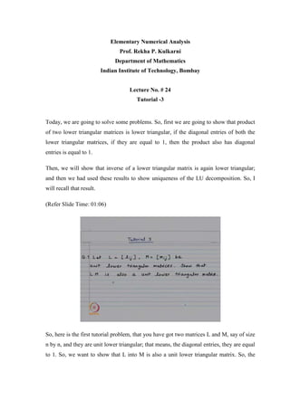
  • 1. Elementary Numerical Analysis Prof. Rekha P. Kulkarni Department of Mathematics Indian Institute of Technology, Bombay Lecture No. # 24 Tutorial -3 Today, we are going to solve some problems. So, first we are going to show that product of two lower triangular matrices is lower triangular, if the diagonal entries of both the lower triangular matrices, if they are equal to 1, then the product also has diagonal entries is equal to 1. Then, we will show that inverse of a lower triangular matrix is again lower triangular; and then we had used these results to show uniqueness of the LU decomposition. So, I will recall that result. (Refer Slide Time: 01:06) So, here is the first tutorial problem, that you have got two matrices L and M, say of size n by n, and they are unit lower triangular; that means, the diagonal entries, they are equal to 1. So, we want to show that L into M is also a unit lower triangular matrix. So, the
  • 2. proof is going to be straight forward, we will just look at the multiplication of these two matrices. (Refer Slide Time: 01:36) The structure of our matrix L is going to be of this form. Along the diagonal, we have got 1, the part which lies below the diagonal it can have non-zero entries or zero entries. But definitely, the elements which are above the diagonal they are going to be 0. So, that means, l ij is equal to 0, if i is less then j, i denotes the row index and j denotes the column index. And l ii is equal to 1 i is equal to 1 2 up to n. Matrix M is going to have similar form and now we look at the product of L into M.
  • 3. (Refer Slide Time: 02:22) So, we have l ij is equal to 0 m ij is equal to 0, if i less then j and l ii is equal to m ii is equal to 1 for i going from 1 2 up to n ijth element of matrix LM. We denote by LM in the bracket i,j. By definition of matrix multiplication, this will be given by summation l ik m kj k goes from 1 to n. So, it is ith row of L multiplied by jth column of m. Now, using the fact that l ij is equal to 0, if i less then j, you are going to have summation k goes from 1 to i, because when k is equal to i plus 1 l ii plus 1 will be 0. So, this is going to be summation k goes from 1 to i l ik m kj. We are interested in the elements of l m, when i is less than j. So, for that case i less than j m kj will be 0 for k going from 1 2 up to i, because for k is equal to 1 2 up to i j will be bigger than k. And m has the property that m ij is 0, if i less than j. And hence this summation… in this summation m kj’s they are going to be 0. So, you get LM i, j is equal to 0. So, as in the case of L and M when you consider the elements LM ij when i less then j they are equal to 0. So, now it remains to show that the diagonal entries they are equal to 1. So, now, we will look at diagonal entry of LM say LM i, i that will be given by ith row of l multiplied by ith column of m.
  • 4. (Refer Slide Time: 04:38) And then we obtain LM i, i to be summation k goes from 1 to n l ik m ki. Now, as before this summation reduces to summation k goes from 1 to i l ik m ki. The only non-zero term in the summation is going to be when k is equal to i. So, you get this to be equal to l ii m ii and this is equal to 1. So, thus product of two lower triangular matrices is going to be a lower triangular matrix and if the diagonal entries of both the matrices they are equal to 1, then the product also has similar property. Now, the next example, which we want to consider is if L is a lower triangular matrix, then its inverse is going to be again a lower triangular. So, you start with a invertible lower triangular matrix and we want to show that its inverse is lower triangular; when we had discussed Gauss elimination method, we had said that finding a inverse using the classical formula is something not advisable, because it is very expensive. So, what one should do is, if one wants to find the inverse of a matrix, then you solve the system Ax is equal to b for right hand side b is equal to e 1, e 2, e n, which are the canonical vectors. And then, when you consider l x is equal to e j, whatever result you get you should write it as a jth column. So, that gives you inverse of A, it is this result we are going to use to show that inverse of a lower triangular matrix is lower triangular
  • 5. (Refer Slide Time: 06:49) The computation of A inverse: A inverse is given by A inverse e 1, A inverse e 2, A inverse e j, A inverse e n . So, the jth column of A inverse is C j, which is equal to A inverse e j equivalently, you get a C j is equal to e jj going from 1 2 up to n. So, thus the column the jth column of A inverse is obtained by solving system of linear equations A C j is equal to e j, where e j is the canonical vector with 1 at jth place and 0 else where. (Refer Slide Time: 07:36) Look at L to be a unit lower triangular matrix, because it is unit lower triangular, determinant of L will be equal to 1. The product of the diagonal entries and hence it will
  • 6. be invertible. Now, we want to show that L inverse is also unit lower triangular. So, you write L inverse as its columns L inverse e 1 L inverse e 2 L inverse e n the jth column C j of L inverse is given by C j is equal to a 1j a 2j a nj, which is equal to L inverse e j. So, that gives you L of c j is equal to e j a, system of equation to solve. (Refer Slide Time: 08:24) Now, our matrix L it has got 1 along the diagonal entries 0 above the diagonal and below diagonal, it is given by this multiplied by say jth column I am denoting the jth column by b 1j b 2j b nj is equal to right hand side, which is ej; So, 1 at jth place and 0 elsewhere. Since the matrix L is lower triangular, we can use forward substitution. So, the first equation has only 1 unknown , but its b 1j and equating you get b 1 j to be 0. Now, second equation will be l 21 b 1j plus b 2j is equal to 0. Now, b 1j is already 0. So, you get the b 2j is equal to 0 and continuing in this fashion, you get b j minus 1 j is equal to 0 when you look at jth equation, the jth equation will be l j1 b 1j l j2 b 2j l jj b jj. Where l jj is going to be 1 and since b 1 j b 2 j b j minus 1 j is equal to 0, you obtain b jj to be equal to 1, if you look at j plus first equation it will have l j plus 1 j b jj plus bj plus 1 j is equal to 0. Now, b jj is equal to 1. So, you are going to get b j plus 1 j is equal to minus l j plus 1 j. So, that is how you can calculate the jth column and in the j th column. The important thing is you get first j minus one entries to be 0, the jth entry to be equal to 1and then remaining entries they may be non-zero or they may be 0.
  • 7. It depends on your matrix l, but definitely in the jth column first j minus 1 entries they are going to be equal to 0 and jth entry is going to be equal to 1. So, that is what will make our inverse to be unit lower triangular. (Refer Slide Time: 10:51) So, when you look at L inverse it is going to have, 1 along the diagonal - star means either it is zero or it is non-zero and above you are getting all 0. So, we get L inverse also to be unit lower triangular. Now, when you look at upper triangular matrices, then whether product of two upper triangular matrices is upper triangular whether inverse of upper triangular matrix is upper triangular. So, the result is true and we can deduce this result for upper triangular matrices by taking the transpose, like we have proved that product of two lower triangular matrices is again a lower triangular. Now, if you are looking at two upper triangular matrices say U 1 and U 2, then when you take transpose, transpose of upper triangular matrix will become lower triangular matrix. So, take the transpose then use the fact that product of two lower triangular matrices is again a lower triangular matrices and then again take the transpose, same idea for showing that inverse of upper triangular matrix is upper triangular. And there we use the fact that the inverse and transpose, these two operations they commute in the sense that a inverse transpose is going to be same as a transpose inverse, whether I take inverse first and then take transpose or take transpose and then take inverse the result is going to be the same.
  • 8. (Refer Slide Time: 12:46) So, let us show this; now, for upper triangular matrices U and V are unit upper triangular take the transpose, then they become unit lower triangular. What we have proved just now is V transpose U transpose that is going to be a unit lower triangular matrix, but V transpose U transpose is nothing but transpose of U into V. So, if U into V transpose is unit lower triangular UV is going to be unit upper triangular. So, U and V unit upper triangular implies their product is also unit upper triangular. For the inverse now, U is unit upper triangular take its transpose it becomes unit lower triangular take its inverse that is going to be unit lower triangular, which we proved just now because the operation of transpose and inverse commute, this will be U inverse transpose. Now, if U inverse transpose is unit lower triangular, then U inverse has to be unit upper triangular.
  • 9. (Refer Slide Time: 13:57) And now using these two results, let us recall the result of uniqueness of LU decomposition. So, if you have A is equal to L 1 U1 is equal to L 2 U 2. Where L 1 and L 2 are unit lower triangular matrices U 1, U 2 are upper triangular matrices and invertible, then from this relation I can deduce that L 2 inverse L 1 is going to be equal to U 2 U 1 inverse I pre-multiply by L 2 inverse and post multiply by U 1 inverse now left hand side is a unit lower triangular matrix right hand side is a upper triangular matrix, if both are equal then both of them they should be diagonal matrix and then because the diagonal entries of L 2 inverse L 1 they are going to be 1, the diagonal matrix is nothing but the identity matrix. So, this is the uniqueness of LU decomposition. So, if a is invertible then A can be written uniquely as L into U, when we proved LU decomposition of the matrix A we had made an additional assumption that look at the principle leadings sub matrix that is formed by first k rows and first k columns of our matrix. So, you take a square matrix, if its determinant is not equal to 0 for k is equal to 1 2 up to n. Then we proved that under this assumption a can be written uniquely as L into U. Now, we want to prove the converse that suppose, A is a invertible matrix and it is given to us that it can be written as L into U. Where L is unit lower triangular, U is upper triangular then we want to show that determinant of a k is not equal to 0. So, thus what we are going to show is if A is invertible you can write a as equal to L into U, if and only if
  • 10. determinant of A k is not equal to 0 for k is equal to 1 2 up to n. Now, in order to prove this result, portioning of this matrix it helps. Let us do one thing, we have got our n by n matrix and we are already considering the leading principles of matrix. So, you have got sub matrix which is formed by first k rows and first k columns. So, look at our remaining sub matrices. (Refer Slide Time: 16:58) So, A is A 11 A 12, A 21 A 22, where A 11 is k by k matrix. So, this A 11 we have been calling it A k; A 12 will be formed by first k rows and next n minus k columns last n minus k columns. So, the size of A 12 is k into k by n minus k matrix A 21 that is formed by n minus k rows and k columns. So, it will be n minus k by k and A 22 will be matrix of size n minus k by n minus k.
  • 11. (Refer Slide Time: 17:44) Next, we look at multiplication of two n by n matrices A and B. So, C is equal to AB then, if you partition matrices AB and C in a similar manner. Then we are going to have C 11 is equal to A 11 B1 plus A 12 B 21, the result is also going to be true for C 12 like C 12 will be given by first row into second column. So, C 12 will be A 11 B 12 plus A 12 B 22 and so, similarly, for C 21 and C 22. So, it is as if we are treating this as 2 by 2 matrix, but for our result we need only the result about C 11. So, let us prove this result. Now, before we proceed notice that C 11is going to be k by k matrix A 11 is k by k B 11 is k by k. So, this is going to be k by k. A 12 is k by n minus k B 21 is n minus k by k. So, when you take their product you again get a k by k matrix. So, in order to prove this result we use the usual formula for matrix multiplication.
  • 12. (Refer Slide Time: 19:28) So, C ij will be given by ith row of a into jth column of b. So, it is summation p goes from 1 to n a ip b p j. This sum I split into two sums p going from 1 to k and p going from k plus 1 to n now you look at. So, our i and j they are going to be lie between one and k. So, 1 less than or equal to i j less than or equal to k then look at a ip. So, i is between 1 and k p is between 1 and k. So, a ip will be nothing but i pth element of A 11 then b pj p is between 1 and k j is between 1 and k. So, b p j will be nothing but B 11 p j plus. Here i is between 1 and k, but p is between k plus 1 to n p means the column. So, that is why this a i p will be i pth element of A 12. So, it is A 12 i p and then b p j. So, b pj will be nothing but p is between k plus 1 to n j is between 1 and k. So, that is B 21 p j. So, this proves C 11 is equal to A 11 B 11 plus A 12 B 21. Now, let us use this fact for lower triangular matrices.
  • 13. (Refer Slide Time: 21:26) So, suppose a is a invertible matrix which is given to us that it can be written as L into U. Let A k denote the principle leadings sub matrix of order k and our claim is that determinant of A k is not equal to 0 for k is equal to 1 2 up to n. (Refer Slide Time: 21:50)
  • 14. So, this is given to us that A is equal to L into U L being a lower triangular matrix with diagonal entries is equal to one determinant of L will be equal to 1. So, determinant of U is equal to determinant of A, which is not equal to 0, because A is given to be invertible matrix. U being an upper triangular matrix determinant of U will be product of the diagonal entries u 11 u 22 u nn and this not equal to 0 implies u ii to be not equal to 0. Now, partition matrix A l and U as before. Because L is lower triangular L 12 is going to be a zero matrix, because U is upper triangular matrix U 21 is going to be a zero matrix. Now, A 11 will be given by L 11 into U 11, because the other L 12 U 21 term both of them they are 0. So, in our notation A k is going to be equal to L k into U k. So, determinant of A k is equal to determinant of U k, because again the diagonal entries of L k is equal to 1 determinant U k is U 11 U 22 U kk which is not equal to 0. (Refer Slide Time: 23:22) And thus we have proved that if A is an invertible matrix, this invertible is important, which can be written as L into U. Then the determinant of the principle leading sub matrix of order k is going to be non-zero for k is equal to 1 2 up to n.
  • 15. (Refer Slide Time: 23:42) Now, as a simple example, let us calculate LU decomposition of this matrix. Now, at this stage I will like to recall that in order to find LU decomposition, what you can do is consider matrix A use Gauss elimination method to reduce it to upper triangular matrix. So, that is going to give you matrix U. And the matrix L will be unit lower triangular - constructed using the multipliers used in the Gauss elimination method. So, we are considering Gauss elimination without partial pivoting when we use gauss elimination with partial pivoting, we get LU decomposition of A. If you are using Gauss elimination with partial pivoting, which involves interchange of rows then LU decomposition is not of the matrix A, but it is the matrix P into A; where P is the permutation matrix obtained by finite number of row interchanges in the identity matrix. So, let us reduce this 3 by 3 matrix to upper triangular form and then find L and U? One can also find directly L and U by multiplying L and U and equating the corresponding entries. But the way I am proving is using Gauss elimination method.
  • 16. (Refer Slide Time: 25:28) So, I want to reduce this to upper triangular form. So, first I want to introduce 0s in the first column, below the diagonal. So, I do second row minus 2 times R 1 and third row minus 3 times R 1. So, our multipliers are 2 and 3. So, they are going to appear in the first column of l. So, the first column of l will consist of 1 here and then these multipliers 2 and 3 when I do these operations these two are 0, then 2 into 2 is 4. So, 5 minus 4 you will get 1 2 into 3 is 6. So, that gives you this entry to be 2 then 8 minus 3 into 2 that will give you 2 and then 14 minus 3 into 3 that will give you 5. So, this is the first stage of Gauss elimination method in the second step you look at the second column and try to make this entry to be 0. So, this can be achieved by R 3 minus 2 times R 2 multiply second row by 2 and subtract from the third row. So, you will get 0 here 2 into 2 is 4; 5 minus 4 this will be 1. Now, the multiplier is 2. So, that is going to occupy this place. So, you will get U to be matrix upper triangular given by here and L to be lower triangular, which is given by this.
  • 17. (Refer Slide Time: 27:03) So, now I want to consider some properties of positive definite matrices; for the positive definite matrix the definition is: it should be a symmetric matrix and x transpose A x should be bigger than 0 for every non-zero vector, now this second property something difficult to verify. For all non-zero vectors we want x transpose A x to be bigger than 0. (Refer Slide Time: 27:42) So, now, we are going to prove a necessary condition that if matrix A is positive definite then its diagonal entries they have to be strictly bigger than 0. So, if you are given a
  • 18. matrix A with one of the diagonal entry to be either a negative real number or 0 then such a matrix cannot be positive definite. Now, for special case of diagonal matrices we are going to show that d is positive definite, if and only if diagonal entries they are bigger than 0 for general matrices it is a necessary condition it is not sufficient that it can happen that diagonal entries are all bigger than 0, but still matrix is not positive definite. But for the diagonal entries they are for the diagonal matrices, it is a necessary and sufficient condition that the entries d ii should be bigger than 0 and proof of both these results they are simple, we are going to use a fact that ei and ej are canonical vectors. So, if I look at e j transpose A e ii get i jth entry of my matrix A. (Refer Slide Time: 29:27) So, the diagonal entries they will be given by e i transpose A e i a is positive definite. So, you look at e i transpose A e i. e i transpose is row vector with one at ith place, A ei is going to be ith column of A. So, it is a 1i a 2i a n i, when i take the multiplications, I get a ii since e i is a non-zero vector and a is positive definite e i transpose a ei is bigger than 0 and hence we get the diagonal entries of a to be bigger than 0. Now, let us look at diagonal matrix.
  • 19. (Refer Slide Time: 30:09) So, suppose D is diagonal matrix with diagonal entries to be d1, d2, d n, we are going to show that this is positive definite if and only if d i is bigger than 0. Now, this way implication that d positive definite implies d i is bigger than 0, this we just now proved for any general matrix. So, it is going to be true for diagonal matrix also. Now, let us look at the converse. So, this is given to us that D is a diagonal matrix d i's are bigger than 0. So, the first thing is d transpose is equal to D and now let us look at x transpose D x, you have got D to be diagonal matrix. So, x transpose D x will be nothing, but summation j goes from 1 to n d j x j square x is a non-zero vector. That means, at least one of the entry is non-zero which will make this sum to be bigger than 0 and that makes diagonal matrix D to be positive definite. I want to consider again Gauss elimination method. So, in the Gauss elimination method, we have proved LU decomposition for example, for positive definite matrices or for diagonally dominant matrices. So, you have got a matrix A, you do the first step of Gauss elimination method and then in the next step you are going to work only on the n minus 1 by n minus 1 sub matrix. So, I start with matrix A to be positive definite, now the next sub matrix, which I am going to work on or after first step of gauss elimination method, whether this property whether it will be preserved.
  • 20. Now, the answer to that is yes, but I am going to prove only the property that if your matrix A is a symmetric matrix, you do first type of the Gauss elimination method and the sub matrix which you are going to work in the next step, it retains the symmetric property. So, it is a important property, because it can help us to reduce our computations by half. (Refer Slide Time: 32:51) So, here is the first type of Gauss elimination method. This is a matrix A and we want to introduce 0s in the first column below the diagonal. So, our multipliers are going to be m i1 is equal to a i1 by a 11and then the operations which we perform are R i becomes R i minus m i1 R 1 multiply the first row R 1 by m i1 and subtract from ith row. When we do this, this is the matrix which we obtain. So, suppose a is symmetric then whether this n minus 1 by n minus 1 sub matrix, which is formed by second, third and nth row and second, third and nth column. So, this matrix is also going to be symmetric this is what we want to show. Now, the modified entries here they are given by a i j modified entry one is equal to a i j minus m i1 a 1j, because this is our operation we are subtracting the first row from the ith row. So, this is what we are doing a ij minus m i one a 1j, a ij will be a entry in the ith row, we consider the corresponding entry in the first row. So, that will be a 1j and multiply by m i1 and subtract.
  • 21. (Refer Slide Time: 34:38) So, our matrix A it becomes a 11 R 1 tilde 0 matrix and A 1, where A 1 is the n minus 1 by m minus 1 sub matrix. (Refer Slide Time: 34:55) This is our question, if A is symmetric then whether A 1 is also symmetric. So, we look at a ij 1 by definitions it is a ij minus m i1 a 1j, what was m i1, it was a i1 by a11. So, I substitute now, I use the fact that A is symmetric; that means, a ij is equal to a ji. So, you get a ji minus a i1 will be same as a 1i, which I am writing here a 1j will be same as a j1, which I am writing here and then a 11.
  • 22. So, you get a ji minus a j1 by a 11 will be nothing but m j1 and then a 1i. Now, this will be nothing but a ji 1. So, thus if your matrix A is symmetric then a1 is also going to be a symmetric matrix. Now, it is also true that if a is positive definite, then a 1 is positive definite if A is diagonally dominant matrix, then A 1 will also be diagonally dominant. So, the matrix is diagonally dominant will mean that we do not have to do row interchanges then then the matrix is positive definite then. In fact, we have seen that we can write its Cholesky decomposition. So, again no row interchanges, we had introduced row interchanges for the sake of stability, when we looked at backward error analysis, we saw that we should not divide by a small number. So, you have to like that is why one considers or it is important that if you do not have to do row interchanges then it is it saves our computational efforts. Now, these two results they are a bit involved. So, I am not going to prove those results, but we are going to consider the effect on the solution if you multiply column of the coefficient matrix by a non-zero number. Look at the system of equations a x is equal to b, in this if I look at a say ith equation and multiply throughout by a non-zero number, then I am not changing the system my solution is going to remain the same. On the other hand, if I multiply column of coefficient matrix by a non-zero number then my solution will be different my system is different, now what we are going to show is that if you multiply jth column of the matrix A by say a number alpha whereas, phi is not equal to 0. The only change in the solution is going to be in the jth component and that jth component gets multiplied by one by alpha our matrix is invertible matrix. If I multiply a column by a non-zero number alpha determinant of the new matrix will get multiplied by alpha. So, if a is invertible my new matrix also will be invertible, because the determinant will be not equal to 0 in doing this, I am changing my system. So, I get a new solution. So, when you compare the new solution with the original solution the only difference will be in the jth component all other components of the original solution and a new solution they are going to be the same. The jth component effect will be what was earlier x j that will become one upon alpha times x j. So, when we consider later on about the scaling of the matrix in order to make it well conditioned, this result is going to be important. Now, the proof of this result is
  • 23. straight forward. What we are going to do is a x is equal to b. So, write xx is our column vector x1,x2, xn this x we can write as x 1 e 1 plus x 2 e 2 plus x n en where e j's are the canonical vector apply a and then see what you get. (Refer Slide Time: 40:49) So, we have a non-singular system; that means, the coefficient matrix A is invertible it is altered by multiplication of its jth column by alpha not equal to 0, then the solution is altered only in the jth component, which is multiplied by 1 by alpha. (Refer Slide Time: 41:13)
  • 24. So, we have got A x is equal to b x is column vector x1, x2, xn this will be equal to x 1e1plus x 2e2 plus xn en. So, when you consider, when you apply A, then Ax will be x1 A e1 plus x2 A e2plus x n A en is equal to b A ej is the jth column, we are going to multiply the jth column by alpha. So, the new system is a tilde which is equal to Ae1 A ej minus 1, these columns they remains as before the jth column becomes alpha times A e j and the j plus first column onwards up to th column they all remain the same. So, now, I can from this relation I can write this as x j by alpha and alpha times A e j. So, I am multiply and divide by alpha. So, I am going to have this is same as equal to b, because in this I am just multiplying and dividing by alpha. So, I will get now this is nothing, but A tilde x tilde is equal to b and what will be x tilde it will be x1 x2 x j minus 1 the jth 1 will be x j by alpha and the last 1 is going to be x n. So, we had original system Ax is equal to b and when you alter it then x tilde which is the new solution it gets altered by only dividing x j by alpha. So, these were some of the problems, which are based on our Gauss elimination method and also on the LU decomposition and in the next tutorial it will be based on norm of a matrix. So, for the gauss elimination method when we want to see the effect of of the perturbation then we need to talk about the norms and the norms come into picture. So, here where some of the problems now about the LU decomposition what you can do is you can try to find LU decomposition directly, you should get the same result and one of the important result which we proved in today’s tutorial is a invertible matrix has LU decomposition if and only if determinant of A k is not equal to 0, where A k is the leading sub matrix, leading principle sub matrix. We had similar result for positive definite matrix; that means, it was the if and only if, result that a is positive definite if and only if you can write a as mm transpose, where M is going to be an invertible matrix. So, thank you.