control systems nptel lecture 48

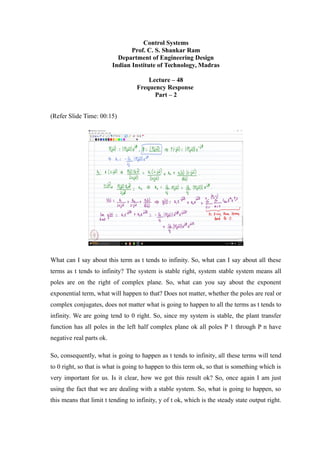
1. Control Systems
Prof. C. S. Shankar Ram
Department of Engineering Design
Indian Institute of Technology, Madras
Lecture – 48
Frequency Response
Part – 2
(Refer Slide Time: 00:15)
What can I say about this term as t tends to infinity. So, what can I say about all these
terms as t tends to infinity? The system is stable right, system stable system means all
poles are on the right of complex plane. So, what can you say about the exponent
exponential term, what will happen to that? Does not matter, whether the poles are real or
complex conjugates, does not matter what is going to happen to all the terms as t tends to
infinity. We are going tend to 0 right. So, since my system is stable, the plant transfer
function has all poles in the left half complex plane ok all poles P 1 through P n have
negative real parts ok.
So, consequently, what is going to happen as t tends to infinity, all these terms will tend
to 0 right, so that is what is going to happen to this term ok, so that is something which is
very important for us. Is it clear, how we got this result ok? So, once again I am just
using the fact that we are dealing with a stable system. So, what is going to happen, so
this means that limit t tending to infinity, y of t ok, which is the steady state output right.

2. So, what is that going to be? It is just going to be a 1 e power minus j omega t plus a 2 e
power j omega t right, because the 3rd set of terms is going to tend to 0 as t tends to
infinity ok. I hope it is clear, how we got this right.
So, now let us substitute for a 1, a 1 is going to be minus U naught divided by 2 j P of j
omega e power j phi, and this multiplied by e power minus j omega t. And plus a 2 is
going to be U naught divided by 2 j the magnitude of P of j omega e power sorry, this is e
power minus j phi, this is going to be e power j phi e power j omega t ok. So, I think I
made another small error here, this should have been e power minus j phi ok sorry,
please go and correct the expression for a 1, that should be minus U naught divided by 2
j magnitude of P of j omega e power minus j phi ok, so that is what we will get right.
(Refer Slide Time: 03:30)
And now, what is e power a times e power b, e power a plus b all right. So, what are we
going to get? So, as a result limit t tending to infinity y of t it is going to be U 0, U
naught is common, magnitude of P of j omega is common. So, what am I left with, I am
left with e power j omega t plus phi minus e power minus j omega t plus phi, the whole
thing divided by 2 j right. So, this implies a limit t tending to infinity y of t is U naught P
of j omega, what is that term in the square bracket? Sin right so, from the Euler’s
relationship right, it is going to be sin of omega t plus phi.
Student: (Refer Time: 04:30).

3. P of minus j omega, P of minus j omega is the magnitude of P of j omega times e power
minus j phi.
Student: (Refer Time: 04:42).
Magnitude, see the magnitude is the same right yeah. So, see because P of minus j omega
will be the magnitude of P of minus j omega e power minus j phi, but the magnitudes
remain the same, it does not matter whether it is P of j omega or P of minus j omega that
is how we got a magnitude of P of j omega to be common, yes, yeah.
Student: as t tends to infinity remain t tends to infinity sin omega t plus while simply
term (Refer Time: 05:09) it oscillates.
Oscillates yeah, so that is what we are finding the limit ok. So, you can converge to a
single value, because it really depends right so what I can say is that this is the function,
to which it oscillates ok. So, as opposed to a unit step response of a stable system in a
unit step response, you will go to a constant value right, for a sinusoidal input, if you
have a stable LTI system, it would be oscillatory ok. It will keep on oscillating that is
what we can that is the frequency response ok, yeah.
Student: So, for a sinusoidal network initially the exponential terms were (Refer Time:
05:46).
Dynamics exactly.
Student: and then
And then, it will ultimately settle down to a sinusoid ok, but there is an important feature
here ok. It will settle down to a sinusoid of the same frequency as that of input ok, we are
just going to look at that here right so let me discuss those points right. So, this is the
expression for the steady state output right so this is the steady state output. Please note
that the steady state output is not a constant value here, but rather it depends on time, but
you it is a what is a sinusoidal pattern right. So, this is the expression for the steady state
output of the system ok.
Now, what is important here? Right so, you look at the frequency, the steady state output
is a sinusoidal what to say a function. But, the frequency of the steady state output is also

4. the same as that of the input ok, so that is an important feature right. So, we immediately
see that the frequency of the steady state output or let me or write it in this way. The
steady state output is a sinusoidal signal of the same frequency as that of the input ok,
but scaled in magnitude by the magnitude of P of j omega, and shifted in phase by phi
ok, which is the phase of P of j omega that is the observation we can make right so from
this derivation right.
Once again, please go through this derivation pretty straightforward. Only thing is that
like instead of numbers, we just worked with general variables, and functions and so on
right, so that is what we did. So, you after the from the derivation, what we can see is
that if you look at the steady state output of this class of systems, the steady state output
is also a sinusoidal signal having the same frequency as the input frequency ok, that is
extremely important ok. However, the steady state output is scaled in magnitude by P of j
omega why, because the magnitude of the steady state output is going to be U naught P
of j, magnitude of P of j omega.
Student: (Refer Time: 09:06)
So, U naught was the magnitude of the input signal right so, P magnitude of P of j omega
is the scaling factor as far as a steady state output magnitude is concerned. And that the
steady state output is shifted in phase by phi right, because phi is the phase of P of j
omega. So, the steady state output is shifted from the input sinusoid by a phase of phi ok,
so that is what we have.
And this is a property of stable linear time in variant systems ok, so that is something
which is very important ok, so that is for stable linear time linear systems. If you give a
sinusoidal input and you wait and measure the steady state output, the steady state output
also will be a sinusoid of the same frequency that is extremely important. And we will
see that we will exploit this fact to discuss methods for the experimental determination of
transfer function ok. And towards the end of this course, we will do a case study right.
So, where I will give you data, and then like you can use these techniques to of
experimentally determine the transfer function ok.
Till now, what the way we have been doing the determination of transfer function is
through analytic means right. So, what did we do, we essentially wrote down equations
of motion governing equations in the form of linear ODEs with constant coefficients.

5. Then we took Laplace transform applied 0 initial conditions, then we calculate at the
transfer function right. So, we will also figure out how to empirically determine that ok
there you will see that the step response and the frequency response are going to play a
vital role ok, when we do that ok, is it clear, what is called as frequency response. So,
this so what is frequency response? Frequency response is nothing but the response of
the system, where to a sinusoidal input that is why it is called frequency response.
And please note that the scaling factor magnitude of P of j omega and the phase shift phi,
which is the phase of P of j omega depend on omega right. Depending on the input
frequencies, these numbers are going to be different ok. So, please remember that ok, so
that is something, which you will address shortly ok yeah. So, this P of j omega is what
is called as a sinusoidal transfer function ok. So, when you when you have P of s, it is a
transfer function right. When you substitute s equals j omega, it essentially becomes a
sinusoidal transfer function ok.
So, how do we get P of j omega, let us say as an example, let us say P of s let us take it as
1 by s plus 1 right, so that is a stable system right. So, then what happens P of j omega
becomes 1 by j omega plus 1, this can be written as 1 minus j omega divided by 1 plus
omega square right by multiplying and dividing by the conjugate right. So, this I can
rewrite as 1 divided by 1 plus omega squared minus j times omega divided by 1 plus
omega square right.
(Refer Slide Time: 12:52)

6. So, consequently what can I have? So, how can I evaluate the magnitude of P of j omega,
I can do square root of real squared plus imaginary squared right. You take the real
component square plus imaginary component square take the add and take the square
root. Alternatively, I can also look at the function ok, if you have a ratio of complex
functions, what is going to be the magnitude? It is going to be the same ratio of the
individual magnitudes right. So, from here, I can immediately rewrite the magnitude of P
of j omega divided to be equal to 1 divided by square root of 1 plus omega square right.
Of course, even if you do real part squared plus imaginary part squared take the square
root, you will get the same answer you can double check ok, so you will get the same
answer. And what is the phase of P of j omega? Once again, you can do tan inverse of
imaginary part by real part or you can just take the what to say algebraic sum of the
individual phases right. So, if the ratio is 1 by j omega plus 1, what will be the phase, the
phase of 1 is 0.
Student: (Refer Time: 14:03).
And then since, what is the phase of j omega plus 1, it is going to be tan inverse of
omega, but that is in the denominator right. So, you have a minus ok so this is going to
be the phase of P of j omega for this example ok, so that is how we calculate the
magnitude and the phase ok. So, once again you know like just as a general what to say
generalization right. So, let us say if P of j omega is going to be n 1 j omega (Refer Time:
14:49) all the way till n m j omega divided by d 1 j omega all the way till d n j omega.
So, what we just did was it like magnitude of P of j omega is essentially going to be just
the same structure, but the individual take the individual magnitudes right, so that is what
we are going to have so it is going to be this. And what about the phase, the phase of P of
j omega is just going to be the algebraic sum, so that is going to be the phase of n 1 j
omega plus all the way till phase of n m j omega minus the phase of d 1 j omega all the
way till the phase of d and j omega ok, so that is what we get right ok, so that is what we
have oops sorry ok, so that is how we calculate the sinusoidal transfer function right.
Now, are there any questions?
Student: (Refer Time: 16:12)

7. Yeah, tan inverse of minus omega, we just write it as minus tan inverse omega right, so
ok, so that is it. Yeah, if you do tan inverse of imaginary by real, you will get tan inverse
of minus omega, you just take it out right. Of course, it is a periodic function right,
depending on how you want rewrite it ok. So, you will see that that is that is exactly my
next point ok. Now, the question is you know like all these equations are fine, so from an
engineering perspective, how are we going to visualize it ok. So that your question leads
to my next topic of discussion, which we are going to continue from tomorrow but I am
going to leave you with one question ok.
So, the questions which I am going to leave you with is the following right. So, how can
one visualize a P of j omega as omega has changed, as omega is varied right. So, because
let us say you know like from a design perspective right, so from an analysis perspective
you know like this fine right. So, we have some expressions, we have some formulae and
so on right. So, I have the plan sinusoidal transfer function as a function of omega and so
on right.
So, now but you see that all these are like as a system order increases, you know like you
are seeing that the sinusoidal transfer function becomes more or more complex in
structure right. So, then you know like how does one interpret right, and use it for design
ok. So, for that prospective from the prospective, you know like it becomes quite
important to figure out, how one can visualize right the sinusoidal transfer functions
variation as omega is vary.
Question is first of all we need to ask ourselves, can we visualize graphically, when this
P of j omega, how P of j omega changes as omega is vary, if so how? And the answer is
yes, we can write and broadly there are three visualizations that typically are used. So,
the first one is what is called as a Bode plot ok, so a Bode plot is one, where there is
something called as a magnitude plot ok. A magnitude plot where the magnitude of P of j
omega is plotted, this is omega ok.
But, of course on a different scale, we will discuss it tomorrow ok. We will use a
logarithmic scale, and a logarithm measure. And we have what is called as a phase plot,
where the phase of P of j omega is plotted against omega ok, so that is the first
visualization ok. Of course, we are going to as I told you we are going to use logarithmic

8. measures and logarithmic scales right. So, we will discuss more about that tomorrow ok.
So, a Bode plot is very commonly used ok.
So, a second visualization is what is called as a Nyquist plot. So, a Nyquist plot is
essentially a plot of the real part of P of j omega, this is the imaginary part of P of j
omega in the complex plane ok. What is called as a P of s plane so right? So, we will see
what this is right, as we go further.
(Refer Slide Time: 20:19)
The 3rd plot is what is called as a Nichols plot ok. So, what is this Nichols plot? I leave it
you as a question ok, just search, and find out and tell me the answer tomorrow ok. So,
by enlarge, we are going to focus on the Bode plot ok. The Bode plot is something,
which you will see that it is very frequently used in engineering applications as far as
studying frequency response is concerned ok, so that is something, which we are going
to concentrate to a great degree.
And we are also going to learn how to use the Bode plot for design purpose ok. So it
does not matter, you know like what is your domain automotive biomedical, you know
like or even other domains right. So, you will see that you know like Bode plot is
something, which is frequently used ok, in the design process.
So, we are going to study Bode plot in detail. A Nyquist plot, and Nichols plot, I will just
explain what it what they are ok, so that will be the extent of essentially discussion that

9. we will do. Because, we want to get into design as using frequency response for which
Bode plot becomes pretty important right. So, we will start with the Bode plot in the next
class and then, we will see how given a transfer function, we can get the Bode plot of
that transfer function ok.
Then you know we will also ask the inverse question, if say through some means I give
you the Bode plot of a system right, which is which can be obtained through experiments
can you figure out the transfer function all right, so that is the inverse question to ask ok.
So given P of s what is a Bode plot that is something, which you will learn and then
given the Bode plot, can you figure out P of s that is a question we will ask ourselves
right, because as an engineer that is pretty important right. So, both problems are both
questions are equally important to us fine right. So, I will stop here, and then like we will
continue from this place tomorrow.