control systems nptel lecture 61

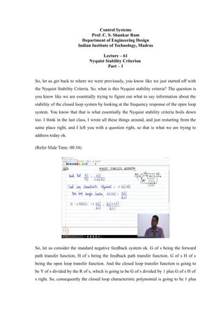
1. Control Systems
Prof. C. S. Shankar Ram
Department of Engineering Design
Indian Institute of Technology, Madras
Lecture – 61
Nyquist Stability Criterion
Part – 1
So, let us get back to where we were previously, you know like we just started off with
the Nyquist Stability Criteria. So, what is this Nyquist stability criteria? The question is
you know like we are essentially trying to figure out what to say information about the
stability of the closed loop system by looking at the frequency response of the open loop
system. You know that that is what essentially the Nyquist stability criteria boils down
too. I think in the last class, I wrote all these things around, and just restarting from the
same place right, and I left you with a question right, so that is what we are trying to
address today ok.
(Refer Slide Time: 00:34)
So, let us consider the standard negative feedback system ok. G of s being the forward
path transfer function, H of s being the feedback path transfer function. G of s H of s
being the open loop transfer function. And the closed loop transfer function is going to
be Y of s divided by the R of s, which is going to be G of s divided by 1 plus G of s H of
s right. So, consequently the closed loop characteristic polynomial is going to be 1 plus

2. G of s H of s. And why is this important, the roots of this closed loop characteristic
polynomial are the closed loop poles right. So, the open loop transfer function G of s H
of s, let us consider it to be represented as n o of s divided by d of s right that is
essentially saying that the open loop transfer function is a ratio of two polynomials in s
right.
So, consequently I can rewrite this a closed loop characteristic polynomial 1 plus G of s
H of s as 1 plus n o of s divided by d o of s, which is d o of s plus n o of s divided by d o
of s ok, so that is what we have. And we are particularly interested in the numerator.
Why, because the roots of the numerator polynomial are the closed loop poles right.
(Refer Slide Time: 02:10)
So, please recall, the zeros of 1 plus G of s H of s are the closed loop poles right, so that
is that is important for us right. So, but the poles of 1 plus G of s H of s are the open loop
poles right. So, why, because if you look at the denominator of the polynomial 1 plus G
of s H of s is d o of s right, d o of s is nothing but the denominator polynomial of the
open loop transfer function. So, consequently you will see that this is going at the poles
of 1 plus G of s H of s are going to be the open loop poles ok, so that is what we have
right, so that is something, which we already identified.
Now, the question that we are asking ourselves the place, where we stopped last class
was it. Can I comment on the location of the closed loop poles, which in turn is a saying

3. that ok. Can I comment on the stability of the closed loop system by plotting the
frequency response of the open loop system ok, or the open loop transfer function right.
So, question is can I plot G of j omega H of j omega has a Nyquist plot right, the Nyquist
plot of that. And then from that comment on the stability of the corresponding closed
loop system ok. That is what that is the question, we have asking ourselves right. So, the
in order to answer that question ok, the first concept we are going to look at is what is
called as a mapping theorem. So, let us look at this theorem ok, so what does this
theorem tell, and how are we going to utilize this theorem for our purpose ok, so that is
something, which we do.
(Refer Slide Time: 03:59)
So, let us go to the handout, you know like which I already shared on the course website
right. So, if you look at this mapping theorem right, so what are we saying. So, let me
essentially read it from here. So, we are saying let F of s be a ratio of two polynomials in
s ok. So, I am discussing this mapping theorem that is what we are discussing right. So,
let F of s be any polynomial a complex valued function right, which is in turn a ratio of
two polynomials in s ok, it has a numerator, and a denominator ok.
Let a closed contour in the s-plane contain is a zeros, and P poles of F of s without
passing over any of the poles and zeros of F of s ok, so that is what we are considering.
So, what I am doing, I am considering a closed contour in a in the s-plane ok, that means

4. that any what to say shape any arbitrary shape that essentially is a contour in the s-plane,
but does not pass over any of the poles or zeros of this function capital F of s.
Then this closed contour in the s-plane is mapped to a corresponding closed contour in
the F of s plane, because see if you have a path in the s-plane of, obviously we are going
to have what to say at each and every point in the contour a particular value of s that
value of s you can substitute in F of s, obviously you will get a corresponding value in
the F of s plane. So, you can map it to the F of s plane right.
So, once we do that what is going to happen, what is going to happen is then we are
going to get a corresponding contour in the F of s plane ok. Then what we do is in the we
count the number of clockwise encirclements of the origin by the contour in the F of s
plane ok. We will see how to close clock on these encircles ok. What is meant by an
encirclement, and how do we count them ok.
So, now, if I count the number of clockwise encirclements of the origin, by the contour in
the F of s plane that is going to be equal to Z minus P ok. What pair is Z and P, Z was the
number of zeros of F of s within the contour in the s plane ok, P was the number of poles
of the function F of s, which was contained within the contour in the s-plane ok. So, Z
minus P would be the total number of clockwise encirclements of the origin in the F of s
plane of the corresponding closed contour right.
(Refer Slide Time: 06:49)

5. So, let me illustrate what this is ok. So, we have read the statement, so let us say we see
what it means right. So, we have a function, so let us say consider a complex valued
function F of s right, so that is what we are essentially doing.
So, what we are saying in the mapping theorem is it. First you give me the s-plane I take
the s-plane ok, and I take any contour let us say any arbitrary contour in the s-plane ok.
This is a closed contour in the s-plane is it not right. So, obviously, the s-plane you need
to mark the number of poles and zeros of F of s right that is what we have been doing till
now right.
So, what this theorem says is that. So, this is going to be mapped into a corresponding
contour in the F of s plane ok. So, let us say you know like some arbitrary contour you
know, let us say for as the sake of argument, let us say F of s as let us say a two poles
here right, and let us say a 0 here ok, so if I take this green contour you know, which
arbitrary drawn right. So, what are the values of Z and P, Z should be the number of
zeros of F of s in the within the contour right, P should be the number of poles of F of s
within the contour. So, in this particular example Z and P are both 0 right.
So, what is going to be the number of encirclements of the origin, it is going to be 0,
because Z minus P right. So, I will have some arbitrary contour in the F of s plane, which
may be like this you know some something like this. I am just drawing an arbitrary
contour ok, so which essentially gets mapped this way ok. This s contour gets mapped to
this F of s plane, and it will be this way ok.
Now, on the other hand, let us say I take a contour you know like which essentially is
like this ok. So, what happens here? So, in this case, Z was 0 and P was 0 rights. In this
case, what happens, what is what are Z and P, Z is 1, P is 2 right within the contour. So,
what is Z minus P minus 1?
So, what does a negative value mean that means that see what was N, N was a number of
clockwise encirclements of the origin, and negative value means you know it is anti-
clockwise or counterclockwise encirclement that is what it is right. So, this black contour
may be mapped to something like this. I am just drawing an arbitrary shape without. So,
you see that if you stand at the origin, it is encircling the origin, ones in the
counterclockwise direction that may be the mapping here ok.

6. So, what this mapping theorem essentially says if you write the mathematical statement,
it essentially says N is equal to Z minus P ok, so that is the equation ok, the mathematical
statement of this mapping theorem ok. It essentially says it look you know like if I have a
closed contour in the s-plane, which does not pass over any of the poles or zeros of F of s
an arbitrary function F of s.
Then that contour in the s-plane gets mapped to a corresponding closed contour in the F
of s plane, and the number of encirclements of that contour in the of s plane in the
clockwise direction N is going to be Z minus P. And what is Z? Z is the number of zeros
of F of s within the closed contour in the s-plane, P is the number of poles within the
closed contour and the s-plane ok, so that is what this mapping theorem is ok. N is equal
to Z minus P ok. So, please remember that yes.
Student: (Refer Time: 11:15) initial contour that you had correction during (Refer Time:
11:19).
Yeah. So, typically you would take a clockwise contour ok. So, yeah it can get mapped to
a clockwise or counterclockwise control like a depending on the function right.
Student: Even that Z (Refer Time: 11:30) that is means that (Refer Time: 11:34).
Z minus P is 0, that means that number of clockwise encirclements or the origin is F of F
of s plane is 0 that is what it is right, so that is what happens right.
Student: (Refer Time: 11:48) circle.
Yeah you can have.
Student: How you (Refer Time: 11:50).
Yeah yeah we we will we are going to look at examples exactly ok. Yes.
Student: What is capital (Refer Time: 11:56)?

7. (Refer Slide Time: 12:30)
Capital N capital N is the let mewrite down the meanings of all these terms ok. So,
capital S is essentially the number of zeros of the function F of s within the closed
contour in the s-plane that is Z ok. What is P? P is the number of poles of F of s that lie
within the closed contour in the s-plane that is P ok. So, N is the number of clockwise
encirclements of the origin in the F of s plane of the origin by the corresponding contour
in the F of s plane right ok.
So, you map a close contour in the s-plane to a corresponding contour in the F of s plane,
and then you get this result ok, so that is a mapping theorem. If the value of N is negative
that means, it is counterclockwise, N is positive means, it is clockwise right. If N is 0,
there is no encirclement ok, so that is what it means ok.
Student: (Refer Time: 13:57) related to the there also Capital N (refer Time: 14:00).
No no no that is the different ok. Good, good point Good point. You know like, so that is
a good observation. So, let me just maybe used use a different N here ok, let me put N c
some N contour right. So, did we used Z and P for something else right. I do not recall
right ok, I hope everyone understood this question you know like, this is not the same
Capital N as we wrote for s power n in type 0, type 1, type 2 system ok, this is different
ok, so that is why I am just putting N c that is why good observation right. Yeah ok.

8. (Refer Slide Time: 14:51)
So, let us look at some examples ok, so that is what I have presented in the handout ok.
In the handout, you know like, essentially what I have done is a following I have just
taken this particular function for F of s oops right. So, essentially one may wonder why
this example has been taken you know, I will explain to you once we discuss ok. So, let
us say you know we take F of s to be this function ok, which has two zeros at minus 1.5
plus or minus 2.4 j right, and two poles at minus 1, and minus 2 right.
(Refer Slide Time: 15:33)

9. Let us look at the function F of s, in that form current t right. Now anyway of course, I
had given the references as ogata ok. So, with this example has been taken from that
book right. So, if you look at the first figure right, so where can you see the two poles,
you know like the two poles all right minus 2 and minus 1 right. So, we already know
that that right.
And the two zeros are at are complex conjugate at these points ok. So, to begin with if
you take a contour A, B, C, D, in the s-plane so happens that if you plot it, I leave it to
you as an exercise ok, to do it in matlab. You take an corresponding contour, this is not a
closed contour by the way ok, we are not analyzing mapping theorem yet right. So, this
is an open contour, if you look at A, B, C, D it is not a closed contour.
You can see that that gets mapped to a contour A prime, B prime, C prime, D prime in
the F of s plane right. So, the corresponding character of the prime is the corresponding
value in the F of s plane right. And we get a different shape altogether right that depends
on the function right. So, similarly if you have the contour D, E, F, A that gets mapped to
a contour D prime, E prime, F prime, A prime ok, so that is how it just turns out right.
(Refer Slide Time: 16:52)
So, now if you take a closed contour A, B, C, D, E, F, A, I hope you do not agrees it that
is a closed contour in the s-plane. Now, you can see that that gets mapped to the contour
A prime, B prime, C prime, D prime, E prime, F prime back to A prime ok, so that is
what happens with this particular contour right. How do you get it, once again you need

10. to plug in and generate the curve ok, and is there a gap between these two curves right
should there be a gap, do you think you know like, when you plot C for example, when
you go from D prime, E prime will it overlap with this part of this B prime. I want you to
figure it as homework ok, so please do it. Then you come back and tell me what your
observations are I hope my question is clear right.
So, you see two for example, arcs, you know like, which seem to have a constant gap in
between right would you have a gap there or would it not be there, if it would not it if it
is not there, what is the reason right. So, I think, you need to figure it ok. Please take this
take an arbitrary contour, and map it right using matlab yes.
Student: How many (Refer Time: 18:12) matlab.
How do we.
Student: Representing something with rectangular (Refer Time: 18:17).
We are just taking a some arbitrary contour ok.
Student: What is contour (Refer Time: 18:21).
Contour, contour is a just a curve right, it is just a domain in the s-plane.
Student: (Refer Time: 18:28) input.
It is not an input per say, it is input to this mapping theorem right, so that is it. So, it will
give you see a what is a set of values of s right put it naught.
Student: What is a (Refer Time: 18:40) a in this case.
A is a point. See A is a point. Let us say you start from 3 s c equals minus 3 is a right that
is it ok. You just draw an arbitrary contour and give some values of.
Student: (Refer Time: 18:53) values.
Yes and then plug into F of s, you know of s already, and then generate that contour in
the F of s plane yes.
Student: How is this (Refer Time: 19:02).

11. We are coming good point. We are going to answer that right. How is this useful, you
know like that is something, which we are going to learn. How are we going to apply to
our subject with this control systems that is a good question, we will come there ok. So,
please bear with me for another five minutes ok, I will explain this.
So, now within this closed contour in the s-plane how many zeros and how many poles
of F of s are present. What are what are the values of Z and P, Z is 0 right, because the
two zeros lie outside right, what is the value of P, two, so what is Z minus P, minus 2.
So, now, you stand at the origin in the F of s plane right, and then start counting the
number of encirclements of the origin as you stand at is the origin in the F of s plane, and
sweep through the entire mapped contour in the F of s plane. So, you look at it you draw
a vector from the origin to A prime, which is your starting point, and then start sweeping.
So, if you come to A prime, B prime, C prime, D prime, you have one encirclement right,
you would have rotated three 360 degrees around the origin in the counterclockwise
direction. Let us not worry about the magnitude, the magnitude changes. But, then the
angle will come to 360 degrees, do you agree?
Now, you go D prime, E prime, F prime, back to A prime, you sweep another 360
degrees right in the counterclockwise directions. So, how many counterclockwise
encirclements do we get? 2 in the F of s plane right. So, what should be the value of N c
minus 2, and that is what you get from the mapping theorem right.
So, the mapping theorem says that N subscript c should be Z minus P. So, Z here in this
example was 0, P is 2. So, Z minus P becomes minus 2, and that is what you can
observed from the diagram in the f of s plane ok. In figure D, if you look at it, the entire
contour has been stretched a little bit, so that you enclose both the zeros within the
contour right. So, now what are the values of Z and P, 2 and 2? So, number of
encirclements should be Z minus P should be 0. So, you look at it, you look at the map
contour in the F of s plane does it encircle the origin, no right. The map contour does not
encircle direction ok, so that is what it is right.

12. (Refer Slide Time: 21:46)
So, there are a few more examples in this case A, B, C, D has only one 0, you can have
contours like this also right, and no poles. So, Z minus P will be 1 here. So, you look at A
prime, B prime, C prime, D prime, it encircles origin once in the clockwise direction,
because N c will be 1 here plus 1 right. So, you can see that A prime, B prime, C prime,
D prime will encircle the origin once in the clockwise direction. If you take E, F, G, H
does not encircle any, it does not contain any of the zeros or poles, it just gets mapped to
E prime, F prime, G prime, H prime ok, so that is what happens right yeah.
Student: (Refer Time: 22:28) if N c equal to Z 3, then instead of just one (Refer Time:
22:36) taking every every s points here in just one.
But, it would have basically encircle the origin three times that is why I am saying please
do it, and convince yourself yeah. So, because we cannot do it by hand right. So, we
need a this particular example you need to use matlab, or any other numerical tool to
generate the contour. So, good point that is why I am saying kindly a program you know,
I am sure you can you guys can do that right. So, just give a sequence of values of s
right, and then take this F of s, calculate F of s plot it in matlab, then you will see how
the contour comes up right.
So, of course, the finer the would say the closer the values of s, the most smoother will
be the profile in the F of s plane right, which you can do numerically, and then like

13. convince yourself right, please do that, you experiment with different contour ok, so that
is a mapping theorem.