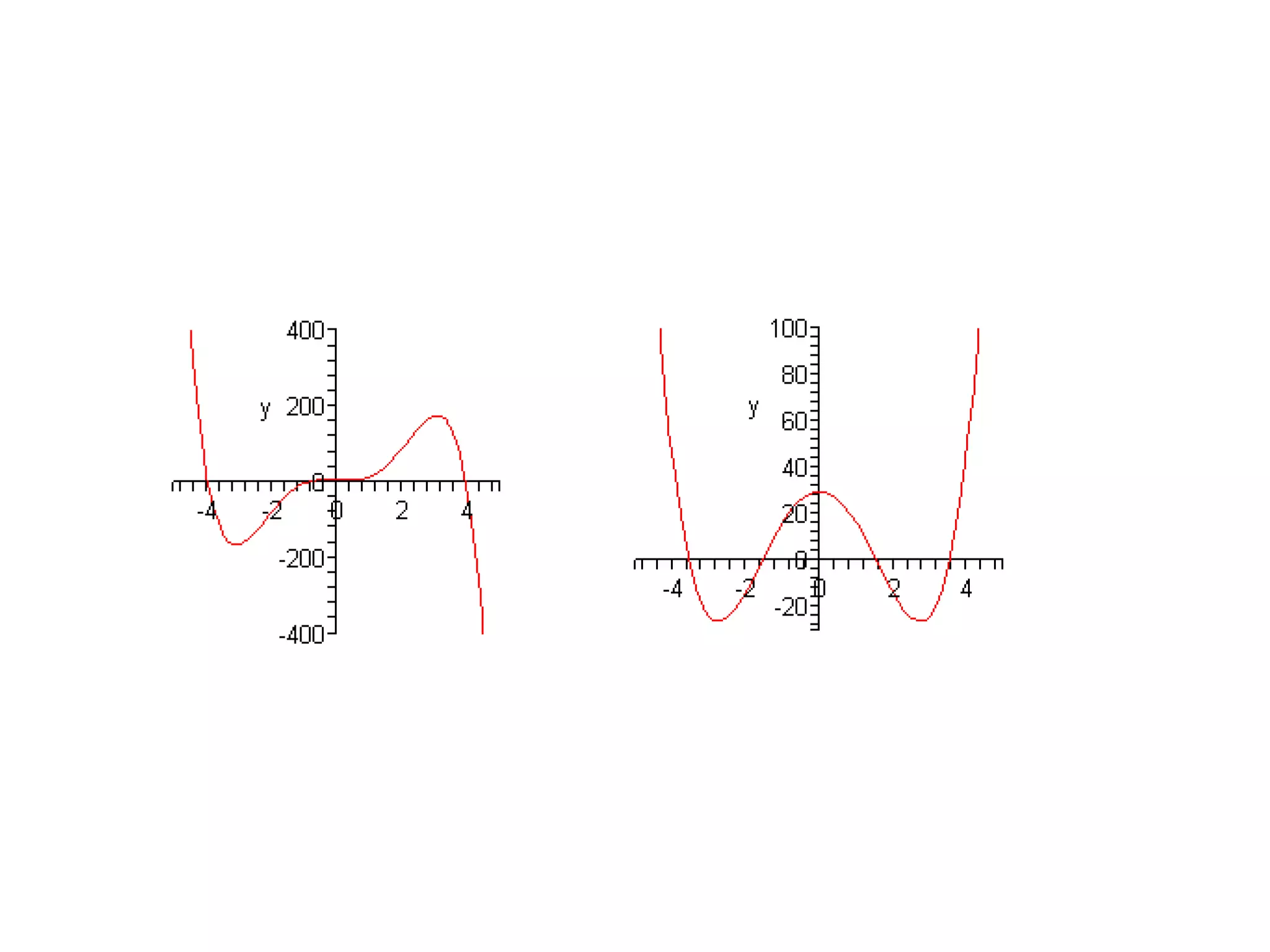
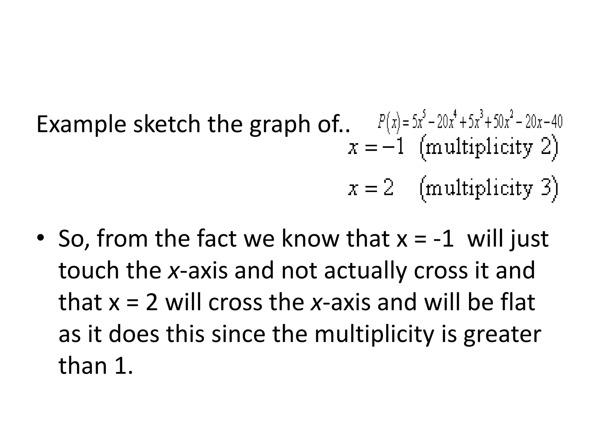
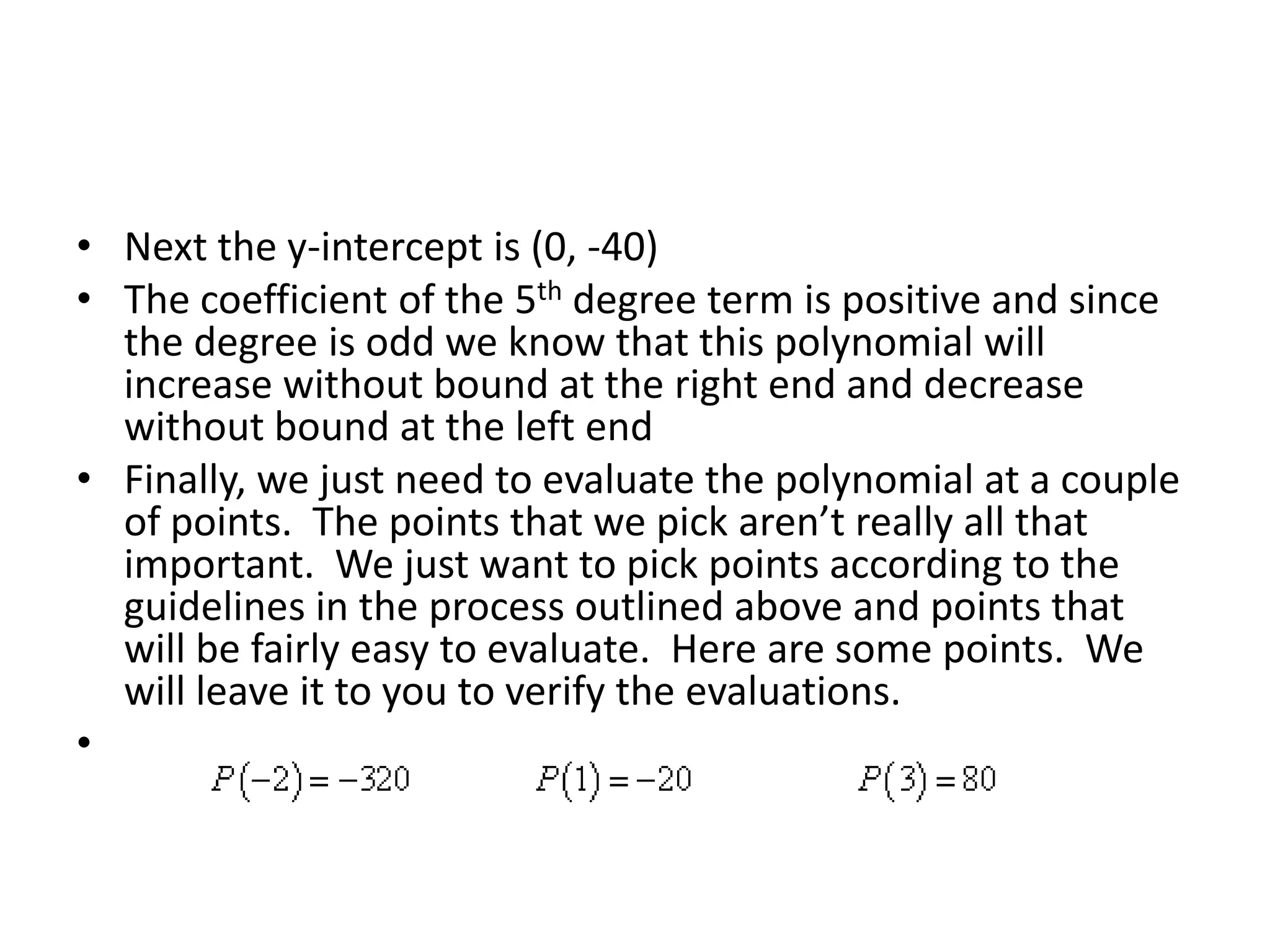
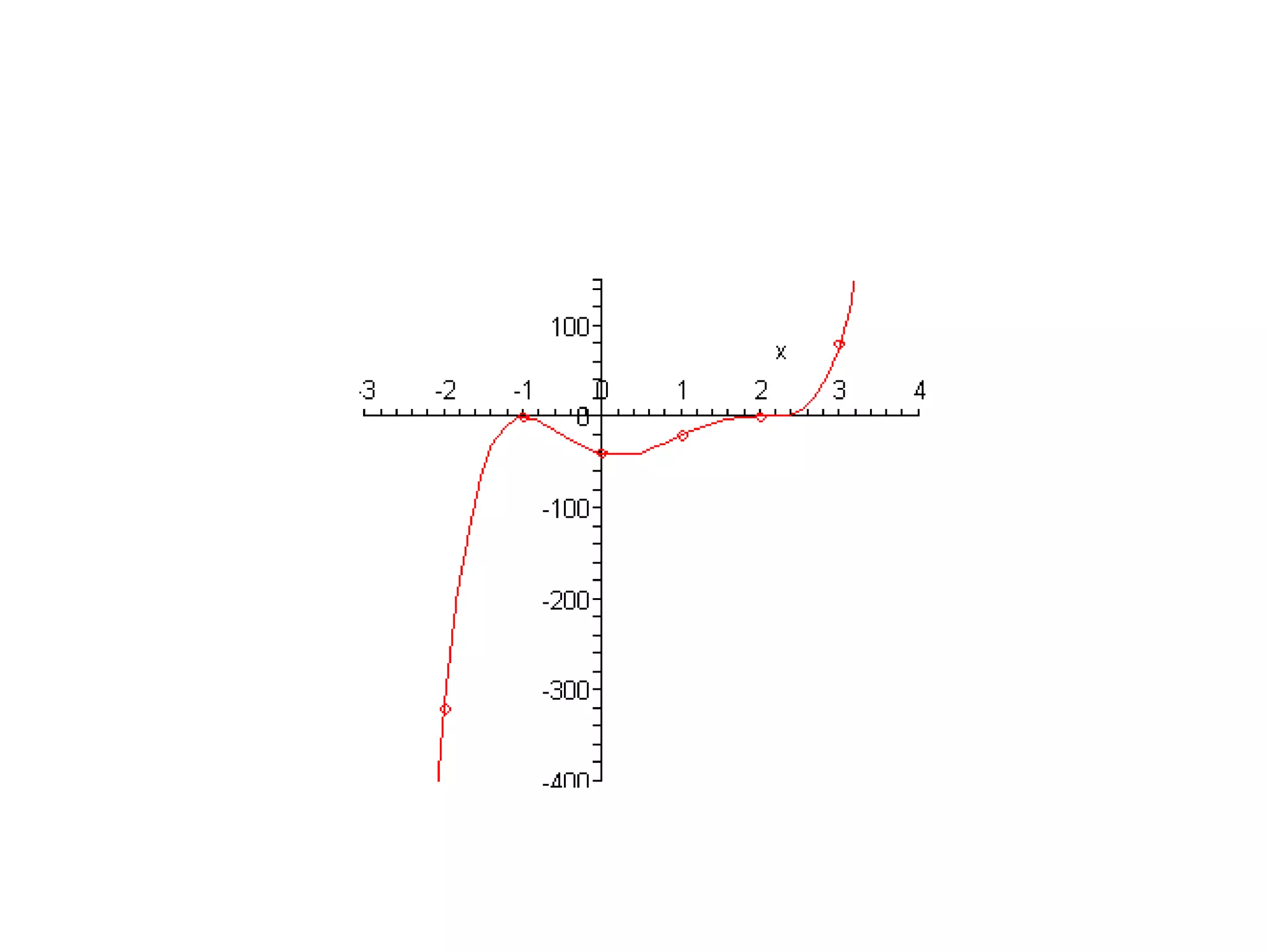
SlideShare a Scribd company logo
1 of 16
Graphing Polynomials	 By MaKenzie Williams
Graphing Polynomials..	 There are  no sharp corners on the graph.. Everything is smooth, it flows through the graph.   The “humps” where the graph changes direction from increasing to decreasing or decreasing to increasing are often called turning points.  If we know that the polynomial has degree n then we will know that there will be at most n - 1 turning points in the graph. 
Next, we need to explore the relationship between the x-intercepts of a graph of a polynomial and the zeroes of the polynomial.  Recall that to find the x-intercepts of a function we need to solve the equation..
Also recall that x = r is a zero of the polynomial P (x), provided P(r) = 0. But this means x = r is also a solution to p (x) = 0. In other words, the zeroes of a polynomial are also the x-intercepts of the graph.  Also, recall that x-intercepts can either cross the x-axis or they can just touch the x-axis without actually crossing the axis.
Notice as well from the graphs above that the x-intercepts can either flatten out as they cross the x-axis or they can go through the x-axis at an angle.
The following fact will relate all of these ideas to the multiplicity of the zero. If x = r is a zero of the polynomial P (x) with multiplicity k then… If k is odd then the x-intercept corresponding to x = r  will cross the x-axis. If k is even then the x-intercept corresponding to x = r will only touch the x-axis and not actually cross it.
Further more if k > 1 then the graph will flatten out at x = r. Finally, notice that as we let x get large in both the positive or negative sense (i.e. at either end of the graph) then the graph will either increase without bound or decrease without bound.  This will always happen with every polynomial and we can use the following test to determine just what will happen at the endpoints of the graph.
Process for Graphing a Polynomial Determine all the zeroes of the polynomial and their multiplicity.  Use the fact above to determine the x-intercept that corresponds to each zero will cross the x-axis or just touch it and if the x-intercept will flatten out or not. Determine the y-intercept,(0 P(0)). Use the leading coefficient test to determine the behavior of the polynomial at the end of the graph. Plot a few more points.  This is left intentionally vague.  The more points that you plot the better the sketch.  At the least you should plot at least one at either end of the graph and at least one point between each pair of zeroe
Example sketch the graph of.. So, from the fact we know that x = -1  will just touch the x-axis and not actually cross it and that x = 2 will cross the x-axis and will be flat as it does this since the multiplicity is greater than 1.
Next the y-intercept is (0, -40) The coefficient of the 5th degree term is positive and since the degree is odd we know that this polynomial will increase without bound at the right end and decrease without bound at the left end Finally, we just need to evaluate the polynomial at a couple of points.  The points that we pick aren’t really all that important.  We just want to pick points according to the guidelines in the process outlined above and points that will be fairly easy to evaluate.  Here are some points.  We will leave it to you to verify the evaluations.  
Now, to actually sketch the graph we’ll start on the left end and work our way across to the right end.  First, we know that on the left end the graph decreases without bound as we make x more and more negative and this agrees with the point that we evaluated at x = -2 .    So, as we move to the right the function will actually be increasing at x = -2 and we will continue to increase until we hit the first x-intercept at  x = 0.  At this point we know that the graph just touches the x-axis without actually crossing it.  This means that at x = 0 the graph must be a turning point.   The graph is now decreasing as we move to the right.  Again, this agrees with the next point that we’ll run across, the y-intercept.  
Now, according to the next point that we’ve got, x = 1, the graph must have another turning point somewhere between x = 0 and x = 1 and  since the graph is higher at x = 1 than at x = 0 .  Just where this turning point will occur is very difficult to determine at this level so we won’t worry about trying to find it.  In fact, determining this point usually requires some Calculus.   So, we are moving to the right and the function is increasing.  The next point that we hit is the x-intercept at x = 2 and this one crosses the x-axis so we know that there won’t be a turning point here as there was at the first x-intercept.  Therefore, the graph will continue to increase through this point until we hit the final point that we evaluated the function at, x = 3.   At this point we’ve hit all the x-intercepts and we know that the graph will increase without bound at the right end and so it looks like all we need to do is sketch in an increasing curve.   Here is a sketch of the polynomial
Note that one of the reasons for plotting points at the ends is to see just how fast the graph is increasing or decreasing.  We can see from the evaluations that the graph is decreasing on the left end much faster than it’s increasing on the right end.
THE END!!! 

More Related Content

What's hot

Calculus
CalculusCalculus
Calculusstudent
 
Lecture 2 ba 2 statistics for business analytics
Lecture 2 ba 2 statistics for business analyticsLecture 2 ba 2 statistics for business analytics
Lecture 2 ba 2 statistics for business analyticsyogesh ingle
 
Graphing inequalities in two variables
Graphing inequalities in two variablesGraphing inequalities in two variables
Graphing inequalities in two variablesJessica Garcia
 
Slope Powerpoint
Slope PowerpointSlope Powerpoint
Slope Powerpointguesta9ee9b
 
Sreb unit2 lesson2
Sreb unit2 lesson2Sreb unit2 lesson2
Sreb unit2 lesson2jpense
 
Question 2
Question 2Question 2
Question 2inner4zn
 
Graphing a line using Slope-Intercept form
Graphing a line using Slope-Intercept formGraphing a line using Slope-Intercept form
Graphing a line using Slope-Intercept formshepieces
 
3.4.08 Limit Intro3
3.4.08   Limit Intro33.4.08   Limit Intro3
3.4.08 Limit Intro3chrismac47
 
All about SAT graphs
All about SAT graphsAll about SAT graphs
All about SAT graphsFabMarks
 
Gauss jordan elimination through pivoting
Gauss jordan elimination through pivotingGauss jordan elimination through pivoting
Gauss jordan elimination through pivotinguis
 

What's hot (20)

Calculus
CalculusCalculus
Calculus
 
Lecture 2 ba 2 statistics for business analytics
Lecture 2 ba 2 statistics for business analyticsLecture 2 ba 2 statistics for business analytics
Lecture 2 ba 2 statistics for business analytics
 
How to
How toHow to
How to
 
Graphing inequalities in two variables
Graphing inequalities in two variablesGraphing inequalities in two variables
Graphing inequalities in two variables
 
Slope Powerpoint
Slope PowerpointSlope Powerpoint
Slope Powerpoint
 
Application of derivatives
Application of derivativesApplication of derivatives
Application of derivatives
 
Unit iii-stability
Unit iii-stabilityUnit iii-stability
Unit iii-stability
 
Sreb unit2 lesson2
Sreb unit2 lesson2Sreb unit2 lesson2
Sreb unit2 lesson2
 
Question 2
Question 2Question 2
Question 2
 
Integers 1
Integers 1Integers 1
Integers 1
 
Graphing a line using Slope-Intercept form
Graphing a line using Slope-Intercept formGraphing a line using Slope-Intercept form
Graphing a line using Slope-Intercept form
 
Solving Linear Equations
Solving Linear EquationsSolving Linear Equations
Solving Linear Equations
 
2.2 slope
2.2 slope2.2 slope
2.2 slope
 
Lec25
Lec25Lec25
Lec25
 
3.4.08 Limit Intro3
3.4.08   Limit Intro33.4.08   Limit Intro3
3.4.08 Limit Intro3
 
All about SAT graphs
All about SAT graphsAll about SAT graphs
All about SAT graphs
 
Presentation 2
Presentation 2Presentation 2
Presentation 2
 
Scatter diagram
Scatter diagramScatter diagram
Scatter diagram
 
Gauss jordan elimination through pivoting
Gauss jordan elimination through pivotingGauss jordan elimination through pivoting
Gauss jordan elimination through pivoting
 
1.2 the normal curve
1.2 the normal curve1.2 the normal curve
1.2 the normal curve
 

Viewers also liked

Media Evaluation Question 3
Media Evaluation Question 3Media Evaluation Question 3
Media Evaluation Question 3zm24
 
Media Evaluation Question 1
Media Evaluation Question 1Media Evaluation Question 1
Media Evaluation Question 1zm24
 
Media Evaluation Question 4
Media Evaluation Question 4Media Evaluation Question 4
Media Evaluation Question 4zm24
 
Media Evaluation Question 2
Media Evaluation Question 2Media Evaluation Question 2
Media Evaluation Question 2zm24
 
Media evaluation intro
Media evaluation introMedia evaluation intro
Media evaluation introzm24
 

Viewers also liked (7)

Media Evaluation Question 3
Media Evaluation Question 3Media Evaluation Question 3
Media Evaluation Question 3
 
Media Evaluation Question 1
Media Evaluation Question 1Media Evaluation Question 1
Media Evaluation Question 1
 
From 0 to 100, TEDx fort wayne and social media
From 0 to 100, TEDx fort wayne and social mediaFrom 0 to 100, TEDx fort wayne and social media
From 0 to 100, TEDx fort wayne and social media
 
Media Evaluation Question 4
Media Evaluation Question 4Media Evaluation Question 4
Media Evaluation Question 4
 
Media Evaluation Question 2
Media Evaluation Question 2Media Evaluation Question 2
Media Evaluation Question 2
 
Media evaluation intro
Media evaluation introMedia evaluation intro
Media evaluation intro
 
Social Media Breakfast Fort Wayne: BIN2011 Wrap up
Social Media Breakfast Fort Wayne: BIN2011 Wrap upSocial Media Breakfast Fort Wayne: BIN2011 Wrap up
Social Media Breakfast Fort Wayne: BIN2011 Wrap up
 

Similar to Graphing polynomials

Graphing rational functions
Graphing rational functionsGraphing rational functions
Graphing rational functionsJessica Garcia
 
Graphing rational functions
Graphing rational functionsGraphing rational functions
Graphing rational functionsJessica Garcia
 
Lecture 13(asymptotes) converted
Lecture 13(asymptotes) convertedLecture 13(asymptotes) converted
Lecture 13(asymptotes) convertedFahadYaqoob5
 
Advanced functions ppt (Chapter 1) part ii
Advanced functions ppt (Chapter 1) part iiAdvanced functions ppt (Chapter 1) part ii
Advanced functions ppt (Chapter 1) part iiTan Yuhang
 
Advanced functions part ii
Advanced functions part iiAdvanced functions part ii
Advanced functions part iiXin Wei
 
14 graphs of factorable rational functions x
14 graphs of factorable rational functions x14 graphs of factorable rational functions x
14 graphs of factorable rational functions xmath260
 
Day 5 examples u5w14
Day 5 examples u5w14Day 5 examples u5w14
Day 5 examples u5w14jchartiersjsd
 
BAS-CAL-LESSON-1-LIMITS-OF-A-FUNCTION.pdf
BAS-CAL-LESSON-1-LIMITS-OF-A-FUNCTION.pdfBAS-CAL-LESSON-1-LIMITS-OF-A-FUNCTION.pdf
BAS-CAL-LESSON-1-LIMITS-OF-A-FUNCTION.pdfostiadess
 
Question 1
Question 1Question 1
Question 1inner4zn
 
Math Lecture 11 (Cartesian Coordinates)
Math Lecture 11 (Cartesian Coordinates)Math Lecture 11 (Cartesian Coordinates)
Math Lecture 11 (Cartesian Coordinates)Osama Zahid
 
1553 linear & quadratic functions
1553 linear & quadratic functions1553 linear & quadratic functions
1553 linear & quadratic functionsDr Fereidoun Dejahang
 
Trigonometry functions of general angles reference angles
Trigonometry functions of general angles reference anglesTrigonometry functions of general angles reference angles
Trigonometry functions of general angles reference anglesJessica Garcia
 

Similar to Graphing polynomials (20)

Graphing rational functions
Graphing rational functionsGraphing rational functions
Graphing rational functions
 
Graphing rational functions
Graphing rational functionsGraphing rational functions
Graphing rational functions
 
M17 t1 notes
M17 t1 notes M17 t1 notes
M17 t1 notes
 
Lecture 13(asymptotes) converted
Lecture 13(asymptotes) convertedLecture 13(asymptotes) converted
Lecture 13(asymptotes) converted
 
Calc 3.5
Calc 3.5Calc 3.5
Calc 3.5
 
1.5 all notes
1.5 all notes1.5 all notes
1.5 all notes
 
Advanced functions ppt (Chapter 1) part ii
Advanced functions ppt (Chapter 1) part iiAdvanced functions ppt (Chapter 1) part ii
Advanced functions ppt (Chapter 1) part ii
 
Advanced functions part ii
Advanced functions part iiAdvanced functions part ii
Advanced functions part ii
 
Calc 3.5
Calc 3.5Calc 3.5
Calc 3.5
 
Calc 3.5
Calc 3.5Calc 3.5
Calc 3.5
 
Calc 1.2a
Calc 1.2aCalc 1.2a
Calc 1.2a
 
14 graphs of factorable rational functions x
14 graphs of factorable rational functions x14 graphs of factorable rational functions x
14 graphs of factorable rational functions x
 
Day 5 examples u5w14
Day 5 examples u5w14Day 5 examples u5w14
Day 5 examples u5w14
 
BAS-CAL-LESSON-1-LIMITS-OF-A-FUNCTION.pdf
BAS-CAL-LESSON-1-LIMITS-OF-A-FUNCTION.pdfBAS-CAL-LESSON-1-LIMITS-OF-A-FUNCTION.pdf
BAS-CAL-LESSON-1-LIMITS-OF-A-FUNCTION.pdf
 
Polynomials lecture
Polynomials lecturePolynomials lecture
Polynomials lecture
 
Question 1
Question 1Question 1
Question 1
 
Math Lecture 11 (Cartesian Coordinates)
Math Lecture 11 (Cartesian Coordinates)Math Lecture 11 (Cartesian Coordinates)
Math Lecture 11 (Cartesian Coordinates)
 
1553 linear & quadratic functions
1553 linear & quadratic functions1553 linear & quadratic functions
1553 linear & quadratic functions
 
Dev project
Dev projectDev project
Dev project
 
Trigonometry functions of general angles reference angles
Trigonometry functions of general angles reference anglesTrigonometry functions of general angles reference angles
Trigonometry functions of general angles reference angles
 

Recently uploaded

Employee wellbeing at the workplace.pptx
Employee wellbeing at the workplace.pptxEmployee wellbeing at the workplace.pptx
Employee wellbeing at the workplace.pptxNirmalaLoungPoorunde1
 
POINT- BIOCHEMISTRY SEM 2 ENZYMES UNIT 5.pptx
POINT- BIOCHEMISTRY SEM 2 ENZYMES UNIT 5.pptxPOINT- BIOCHEMISTRY SEM 2 ENZYMES UNIT 5.pptx
POINT- BIOCHEMISTRY SEM 2 ENZYMES UNIT 5.pptxSayali Powar
 
URLs and Routing in the Odoo 17 Website App
URLs and Routing in the Odoo 17 Website AppURLs and Routing in the Odoo 17 Website App
URLs and Routing in the Odoo 17 Website AppCeline George
 
Concept of Vouching. B.Com(Hons) /B.Compdf
Concept of Vouching. B.Com(Hons) /B.CompdfConcept of Vouching. B.Com(Hons) /B.Compdf
Concept of Vouching. B.Com(Hons) /B.CompdfUmakantAnnand
 
SOCIAL AND HISTORICAL CONTEXT - LFTVD.pptx
SOCIAL AND HISTORICAL CONTEXT - LFTVD.pptxSOCIAL AND HISTORICAL CONTEXT - LFTVD.pptx
SOCIAL AND HISTORICAL CONTEXT - LFTVD.pptxiammrhaywood
 
Organic Name Reactions for the students and aspirants of Chemistry12th.pptx
Organic Name Reactions  for the students and aspirants of Chemistry12th.pptxOrganic Name Reactions  for the students and aspirants of Chemistry12th.pptx
Organic Name Reactions for the students and aspirants of Chemistry12th.pptxVS Mahajan Coaching Centre
 
Paris 2024 Olympic Geographies - an activity
Paris 2024 Olympic Geographies - an activityParis 2024 Olympic Geographies - an activity
Paris 2024 Olympic Geographies - an activityGeoBlogs
 
mini mental status format.docx
mini    mental       status     format.docxmini    mental       status     format.docx
mini mental status format.docxPoojaSen20
 
ECONOMIC CONTEXT - LONG FORM TV DRAMA - PPT
ECONOMIC CONTEXT - LONG FORM TV DRAMA - PPTECONOMIC CONTEXT - LONG FORM TV DRAMA - PPT
ECONOMIC CONTEXT - LONG FORM TV DRAMA - PPTiammrhaywood
 
Crayon Activity Handout For the Crayon A
Crayon Activity Handout For the Crayon ACrayon Activity Handout For the Crayon A
Crayon Activity Handout For the Crayon AUnboundStockton
 
How to Make a Pirate ship Primary Education.pptx
How to Make a Pirate ship Primary Education.pptxHow to Make a Pirate ship Primary Education.pptx
How to Make a Pirate ship Primary Education.pptxmanuelaromero2013
 
The basics of sentences session 2pptx copy.pptx
The basics of sentences session 2pptx copy.pptxThe basics of sentences session 2pptx copy.pptx
The basics of sentences session 2pptx copy.pptxheathfieldcps1
 
Mastering the Unannounced Regulatory Inspection
Mastering the Unannounced Regulatory InspectionMastering the Unannounced Regulatory Inspection
Mastering the Unannounced Regulatory InspectionSafetyChain Software
 
Software Engineering Methodologies (overview)
Software Engineering Methodologies (overview)Software Engineering Methodologies (overview)
Software Engineering Methodologies (overview)eniolaolutunde
 
Introduction to ArtificiaI Intelligence in Higher Education
Introduction to ArtificiaI Intelligence in Higher EducationIntroduction to ArtificiaI Intelligence in Higher Education
Introduction to ArtificiaI Intelligence in Higher Educationpboyjonauth
 
KSHARA STURA .pptx---KSHARA KARMA THERAPY (CAUSTIC THERAPY)————IMP.OF KSHARA ...
KSHARA STURA .pptx---KSHARA KARMA THERAPY (CAUSTIC THERAPY)————IMP.OF KSHARA ...KSHARA STURA .pptx---KSHARA KARMA THERAPY (CAUSTIC THERAPY)————IMP.OF KSHARA ...
KSHARA STURA .pptx---KSHARA KARMA THERAPY (CAUSTIC THERAPY)————IMP.OF KSHARA ...M56BOOKSTORE PRODUCT/SERVICE
 
“Oh GOSH! Reflecting on Hackteria's Collaborative Practices in a Global Do-It...
“Oh GOSH! Reflecting on Hackteria's Collaborative Practices in a Global Do-It...“Oh GOSH! Reflecting on Hackteria's Collaborative Practices in a Global Do-It...
“Oh GOSH! Reflecting on Hackteria's Collaborative Practices in a Global Do-It...Marc Dusseiller Dusjagr
 
Sanyam Choudhary Chemistry practical.pdf
Sanyam Choudhary Chemistry practical.pdfSanyam Choudhary Chemistry practical.pdf
Sanyam Choudhary Chemistry practical.pdfsanyamsingh5019
 
Call Girls in Dwarka Mor Delhi Contact Us 9654467111
Call Girls in Dwarka Mor Delhi Contact Us 9654467111Call Girls in Dwarka Mor Delhi Contact Us 9654467111
Call Girls in Dwarka Mor Delhi Contact Us 9654467111Sapana Sha
 

Recently uploaded (20)

Employee wellbeing at the workplace.pptx
Employee wellbeing at the workplace.pptxEmployee wellbeing at the workplace.pptx
Employee wellbeing at the workplace.pptx
 
POINT- BIOCHEMISTRY SEM 2 ENZYMES UNIT 5.pptx
POINT- BIOCHEMISTRY SEM 2 ENZYMES UNIT 5.pptxPOINT- BIOCHEMISTRY SEM 2 ENZYMES UNIT 5.pptx
POINT- BIOCHEMISTRY SEM 2 ENZYMES UNIT 5.pptx
 
URLs and Routing in the Odoo 17 Website App
URLs and Routing in the Odoo 17 Website AppURLs and Routing in the Odoo 17 Website App
URLs and Routing in the Odoo 17 Website App
 
Concept of Vouching. B.Com(Hons) /B.Compdf
Concept of Vouching. B.Com(Hons) /B.CompdfConcept of Vouching. B.Com(Hons) /B.Compdf
Concept of Vouching. B.Com(Hons) /B.Compdf
 
SOCIAL AND HISTORICAL CONTEXT - LFTVD.pptx
SOCIAL AND HISTORICAL CONTEXT - LFTVD.pptxSOCIAL AND HISTORICAL CONTEXT - LFTVD.pptx
SOCIAL AND HISTORICAL CONTEXT - LFTVD.pptx
 
Organic Name Reactions for the students and aspirants of Chemistry12th.pptx
Organic Name Reactions  for the students and aspirants of Chemistry12th.pptxOrganic Name Reactions  for the students and aspirants of Chemistry12th.pptx
Organic Name Reactions for the students and aspirants of Chemistry12th.pptx
 
Paris 2024 Olympic Geographies - an activity
Paris 2024 Olympic Geographies - an activityParis 2024 Olympic Geographies - an activity
Paris 2024 Olympic Geographies - an activity
 
mini mental status format.docx
mini    mental       status     format.docxmini    mental       status     format.docx
mini mental status format.docx
 
ECONOMIC CONTEXT - LONG FORM TV DRAMA - PPT
ECONOMIC CONTEXT - LONG FORM TV DRAMA - PPTECONOMIC CONTEXT - LONG FORM TV DRAMA - PPT
ECONOMIC CONTEXT - LONG FORM TV DRAMA - PPT
 
Crayon Activity Handout For the Crayon A
Crayon Activity Handout For the Crayon ACrayon Activity Handout For the Crayon A
Crayon Activity Handout For the Crayon A
 
How to Make a Pirate ship Primary Education.pptx
How to Make a Pirate ship Primary Education.pptxHow to Make a Pirate ship Primary Education.pptx
How to Make a Pirate ship Primary Education.pptx
 
The basics of sentences session 2pptx copy.pptx
The basics of sentences session 2pptx copy.pptxThe basics of sentences session 2pptx copy.pptx
The basics of sentences session 2pptx copy.pptx
 
Mastering the Unannounced Regulatory Inspection
Mastering the Unannounced Regulatory InspectionMastering the Unannounced Regulatory Inspection
Mastering the Unannounced Regulatory Inspection
 
Software Engineering Methodologies (overview)
Software Engineering Methodologies (overview)Software Engineering Methodologies (overview)
Software Engineering Methodologies (overview)
 
Introduction to ArtificiaI Intelligence in Higher Education
Introduction to ArtificiaI Intelligence in Higher EducationIntroduction to ArtificiaI Intelligence in Higher Education
Introduction to ArtificiaI Intelligence in Higher Education
 
KSHARA STURA .pptx---KSHARA KARMA THERAPY (CAUSTIC THERAPY)————IMP.OF KSHARA ...
KSHARA STURA .pptx---KSHARA KARMA THERAPY (CAUSTIC THERAPY)————IMP.OF KSHARA ...KSHARA STURA .pptx---KSHARA KARMA THERAPY (CAUSTIC THERAPY)————IMP.OF KSHARA ...
KSHARA STURA .pptx---KSHARA KARMA THERAPY (CAUSTIC THERAPY)————IMP.OF KSHARA ...
 
Model Call Girl in Tilak Nagar Delhi reach out to us at 🔝9953056974🔝
Model Call Girl in Tilak Nagar Delhi reach out to us at 🔝9953056974🔝Model Call Girl in Tilak Nagar Delhi reach out to us at 🔝9953056974🔝
Model Call Girl in Tilak Nagar Delhi reach out to us at 🔝9953056974🔝
 
“Oh GOSH! Reflecting on Hackteria's Collaborative Practices in a Global Do-It...
“Oh GOSH! Reflecting on Hackteria's Collaborative Practices in a Global Do-It...“Oh GOSH! Reflecting on Hackteria's Collaborative Practices in a Global Do-It...
“Oh GOSH! Reflecting on Hackteria's Collaborative Practices in a Global Do-It...
 
Sanyam Choudhary Chemistry practical.pdf
Sanyam Choudhary Chemistry practical.pdfSanyam Choudhary Chemistry practical.pdf
Sanyam Choudhary Chemistry practical.pdf
 
Call Girls in Dwarka Mor Delhi Contact Us 9654467111
Call Girls in Dwarka Mor Delhi Contact Us 9654467111Call Girls in Dwarka Mor Delhi Contact Us 9654467111
Call Girls in Dwarka Mor Delhi Contact Us 9654467111
 

Graphing polynomials

  • 1. Graphing Polynomials By MaKenzie Williams
  • 2. Graphing Polynomials.. There are no sharp corners on the graph.. Everything is smooth, it flows through the graph.   The “humps” where the graph changes direction from increasing to decreasing or decreasing to increasing are often called turning points.  If we know that the polynomial has degree n then we will know that there will be at most n - 1 turning points in the graph. 
  • 3. Next, we need to explore the relationship between the x-intercepts of a graph of a polynomial and the zeroes of the polynomial.  Recall that to find the x-intercepts of a function we need to solve the equation..
  • 4. Also recall that x = r is a zero of the polynomial P (x), provided P(r) = 0. But this means x = r is also a solution to p (x) = 0. In other words, the zeroes of a polynomial are also the x-intercepts of the graph.  Also, recall that x-intercepts can either cross the x-axis or they can just touch the x-axis without actually crossing the axis.
  • 5.
  • 6. Notice as well from the graphs above that the x-intercepts can either flatten out as they cross the x-axis or they can go through the x-axis at an angle.
  • 7. The following fact will relate all of these ideas to the multiplicity of the zero. If x = r is a zero of the polynomial P (x) with multiplicity k then… If k is odd then the x-intercept corresponding to x = r  will cross the x-axis. If k is even then the x-intercept corresponding to x = r will only touch the x-axis and not actually cross it.
  • 8. Further more if k > 1 then the graph will flatten out at x = r. Finally, notice that as we let x get large in both the positive or negative sense (i.e. at either end of the graph) then the graph will either increase without bound or decrease without bound.  This will always happen with every polynomial and we can use the following test to determine just what will happen at the endpoints of the graph.
  • 9. Process for Graphing a Polynomial Determine all the zeroes of the polynomial and their multiplicity.  Use the fact above to determine the x-intercept that corresponds to each zero will cross the x-axis or just touch it and if the x-intercept will flatten out or not. Determine the y-intercept,(0 P(0)). Use the leading coefficient test to determine the behavior of the polynomial at the end of the graph. Plot a few more points.  This is left intentionally vague.  The more points that you plot the better the sketch.  At the least you should plot at least one at either end of the graph and at least one point between each pair of zeroe
  • 10. Example sketch the graph of.. So, from the fact we know that x = -1  will just touch the x-axis and not actually cross it and that x = 2 will cross the x-axis and will be flat as it does this since the multiplicity is greater than 1.
  • 11. Next the y-intercept is (0, -40) The coefficient of the 5th degree term is positive and since the degree is odd we know that this polynomial will increase without bound at the right end and decrease without bound at the left end Finally, we just need to evaluate the polynomial at a couple of points.  The points that we pick aren’t really all that important.  We just want to pick points according to the guidelines in the process outlined above and points that will be fairly easy to evaluate.  Here are some points.  We will leave it to you to verify the evaluations.  
  • 12. Now, to actually sketch the graph we’ll start on the left end and work our way across to the right end.  First, we know that on the left end the graph decreases without bound as we make x more and more negative and this agrees with the point that we evaluated at x = -2 .    So, as we move to the right the function will actually be increasing at x = -2 and we will continue to increase until we hit the first x-intercept at  x = 0.  At this point we know that the graph just touches the x-axis without actually crossing it.  This means that at x = 0 the graph must be a turning point.   The graph is now decreasing as we move to the right.  Again, this agrees with the next point that we’ll run across, the y-intercept.  
  • 13. Now, according to the next point that we’ve got, x = 1, the graph must have another turning point somewhere between x = 0 and x = 1 and  since the graph is higher at x = 1 than at x = 0 .  Just where this turning point will occur is very difficult to determine at this level so we won’t worry about trying to find it.  In fact, determining this point usually requires some Calculus.   So, we are moving to the right and the function is increasing.  The next point that we hit is the x-intercept at x = 2 and this one crosses the x-axis so we know that there won’t be a turning point here as there was at the first x-intercept.  Therefore, the graph will continue to increase through this point until we hit the final point that we evaluated the function at, x = 3.   At this point we’ve hit all the x-intercepts and we know that the graph will increase without bound at the right end and so it looks like all we need to do is sketch in an increasing curve.   Here is a sketch of the polynomial
  • 14.
  • 15. Note that one of the reasons for plotting points at the ends is to see just how fast the graph is increasing or decreasing.  We can see from the evaluations that the graph is decreasing on the left end much faster than it’s increasing on the right end.