Downloaded 59 times

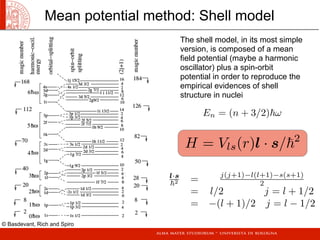
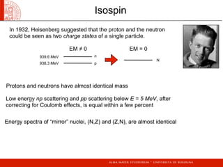
![mN c2
= mAc2
− Zmec2
+
Z
i=1
Bi mAc2
− Zmec2
B = (Zmp + Nmn) c2
− mN c2
[Zmp + Nmn − (mA − Zme)] c2
B =
Zm( 1
H) + Nmn − m( A
X)
c2
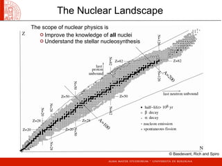
Binding energy
Electrons Mass (~Z)
Atomic Mass Electrons Binding Energies
(negligible)
© Basdevant, Rich and Spiro](https://image.slidesharecdn.com/nucleare2012-161229182603/85/Basics-Nuclear-Physics-concepts-6-320.jpg)
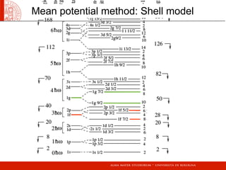
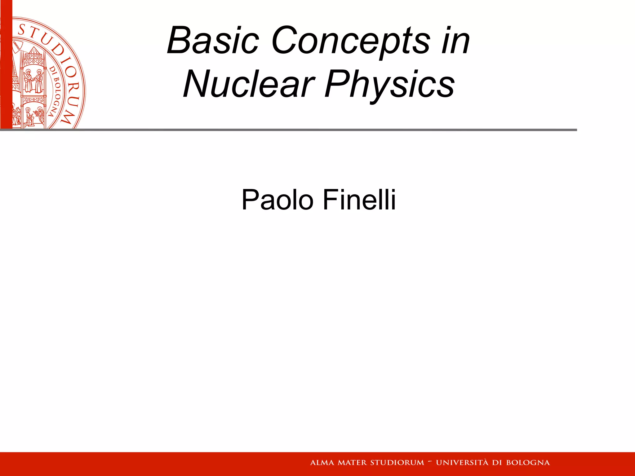
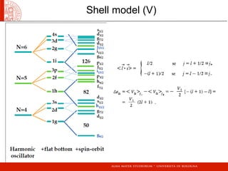
![1F1 (−n, µ + 1, z) =
Γ(n + 1)Γ(µ + 1)
Γ(n + µ + 1)
Lµ
n(z)
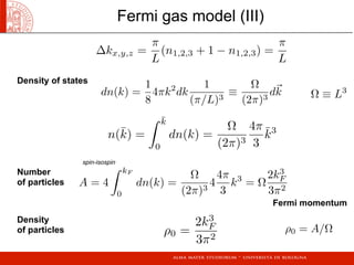
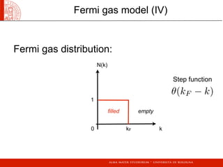
EN =
N +
3
2
ω0 N = 2n + l
d = 2
N
l=0
(2l + 1) = 2
[N/2]
n=0
(2(N − 2n) + 1) =
= 2(2N + 1)
N
2
+ 1
− 8
[N/2]
n=0
d = (N + 1)(N + 2)
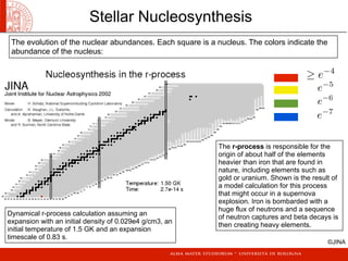
Shell model (II)
Degeneracy](https://image.slidesharecdn.com/nucleare2012-161229182603/85/Basics-Nuclear-Physics-concepts-24-320.jpg)
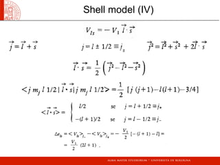
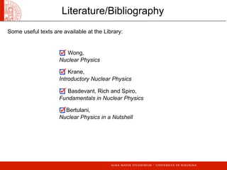
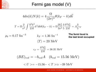
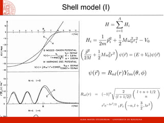
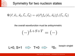
![τ3|π = |π
τ3|ν = −|π
ψN = a|π + b|ν =
a
b
[ti, tj] = iijktk
Pp = 1+τ3
2 =
ˆQ
e
Pn = 1−τ3
2
τ1, τ2, τ3
ti =
1
2
τi
t+|ν = |π
t−|π = |ν
t+|π = 0
t−|ν = 0
t± = t1 ± it2
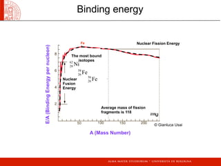
Isospin
eigenstates of the third component of isospin
In general
The isospin generators
Projectors Raising and lowering operators
Pauli matrices
neutron to
proton proton to
neutron
Fundamental representations](https://image.slidesharecdn.com/nucleare2012-161229182603/85/Basics-Nuclear-Physics-concepts-31-320.jpg)
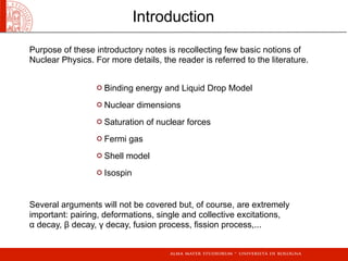
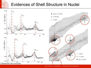
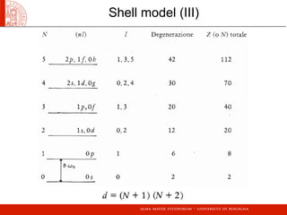
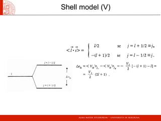
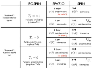
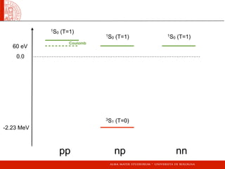
![T = t1 + t2 T = 0, 1
T = 0 η0,0 = 1√
2
(π1ν2 − ν1π2)
T = 1
η1,1 = π1π2
η1,−1 = ν1ν2
η1,0 = 1√
2
(π1ν2 + π2ν1)
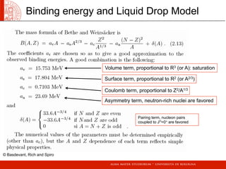
Isospin for 2 nucleons
|T = 1, Tz = 1 = |pp
|T = 1, Tz = −1 = |nn
1
√
2
[|T = 1, Tz = 0 + |T = 0, Tz = 0] = |pn
Proton-proton state
Neutron-neutron state
Proton-neutron state](https://image.slidesharecdn.com/nucleare2012-161229182603/85/Basics-Nuclear-Physics-concepts-32-320.jpg)

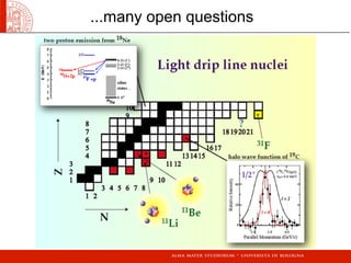
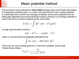

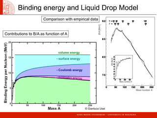
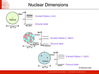
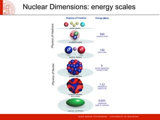
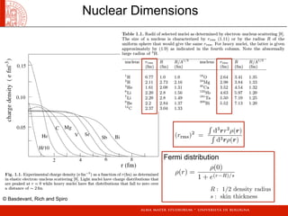
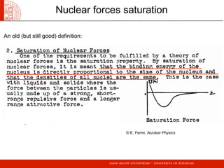
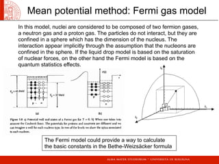
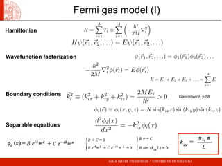
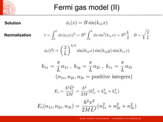
The document provides an introduction to basic concepts in nuclear physics, including: - Binding energy and the liquid drop model, which describes the saturation of nuclear forces. - Nuclear dimensions and the different energy scales involved. - The Fermi gas model, which treats nuclei as two fermion gases and can provide constants for binding energy formulas. - The shell model, which incorporates a mean field potential and spin-orbit potential to reproduce shell structure in nuclei. - Isospin, which treats protons and neutrons as states of a single particle to explain similarities in their behavior.