The document discusses recent advancements in crop classification, focusing on challenges such as limited training data and spatial homogeneity. It presents innovative solutions including semi-supervised learning, spatial classification, and multi-view learning to improve classification accuracy for remote sensing data. Conclusions highlight ongoing work in transfer learning and semantic classification, addressing the complexities of spatiotemporal data.

1. Recent Advances in Crop
Classification
Raju Vatsavai
(vatsavairr@ornl.gov)
Computational Sciences and
Engineering Division
ORNL, Oak Ridge, TN, USA
Collaborators:
B. Bhaduri, V. Chandola, G. Jun, J.
Ghosh, S. Shekhar, T. Burk
Remote Sensing – Beyond Images
Workshop, Mexico
th December, 2013.
City, Mexico, 14
Managed by UT-Battelle
for the Department of Energy

2. Outline
Better spectral and spatial resolution
– Fine-grained (species) classification
– Complex (compound) object recognition
Challenges
– Limited ground-truth: Semi-supervised learning (SSL)
– Spatial homogeneity: SSL + Markov Random Fields
– Spatial heterogeneity: Gaussian Process (GP) learning
– Aggregate vs. Subclasses: Fine-grained classification
– Phenology: Multi-view learning
Conclusions
2
Managed by UT-Battelle
for the Department of Energy

3. Challenge 1: Limited Training Data
Increasing spectral resolution: 4 to 224 Bands
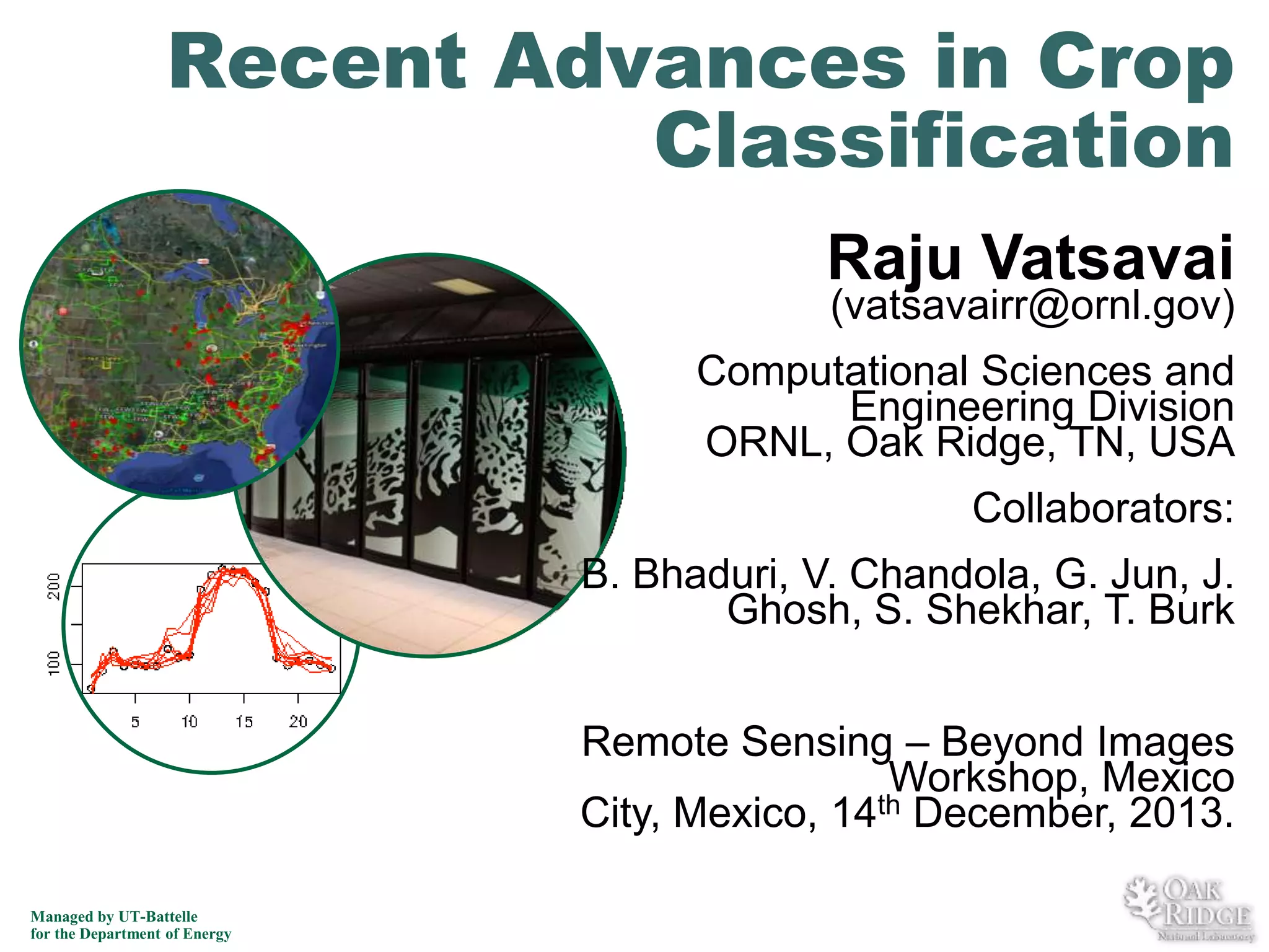
Challenges
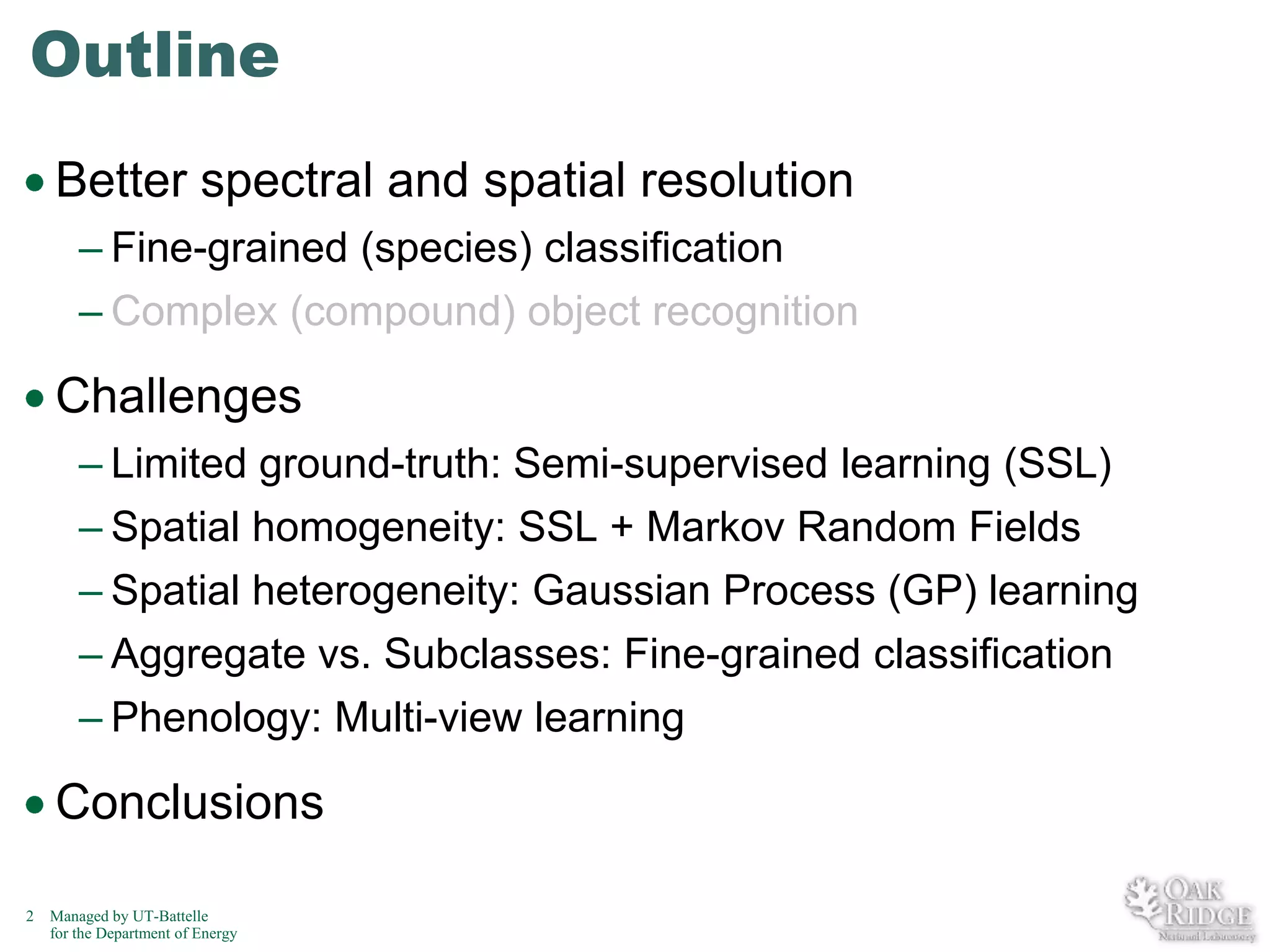
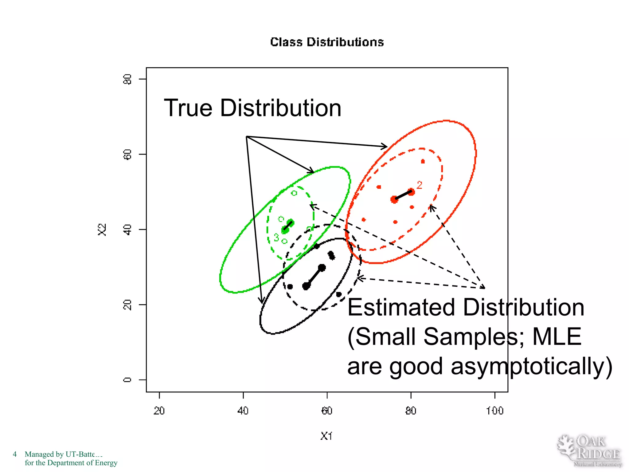
– #of training samples ~ (10 to 30) * (number of dimensions)
– Costly ~ $500-$800 per plot (depends on geographic area)
– Accessibility – Private/Privacy issues (e.g., USFS may average 5%
denied access)
– Real-time – Emergency situations, such as, forest fires, floods
Solutions
– Reduce number of dimensions
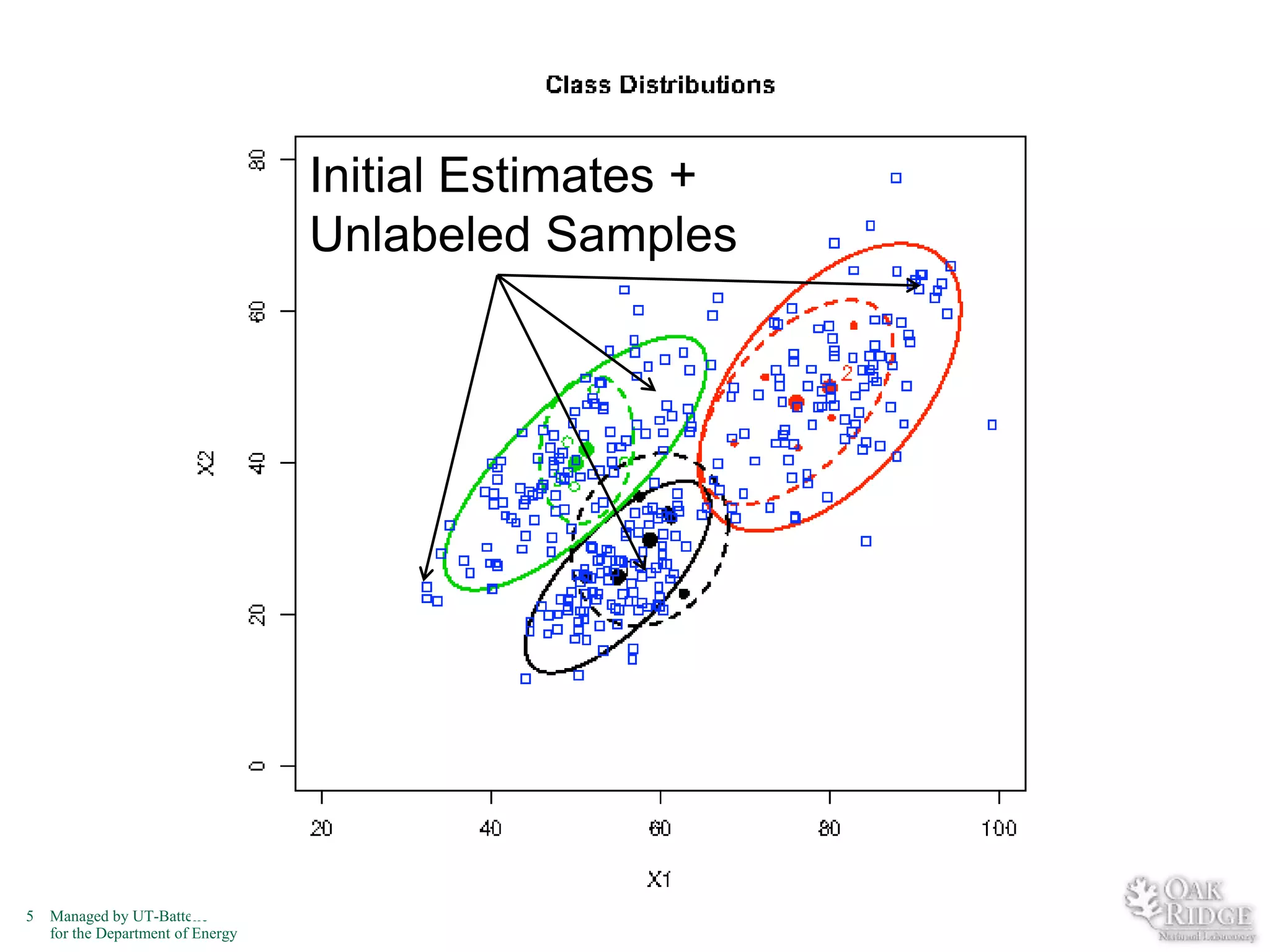
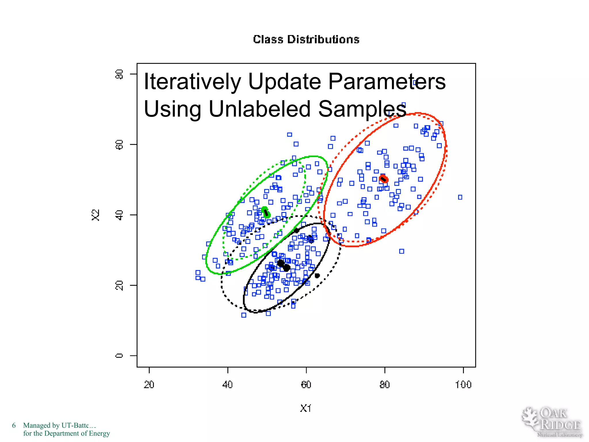
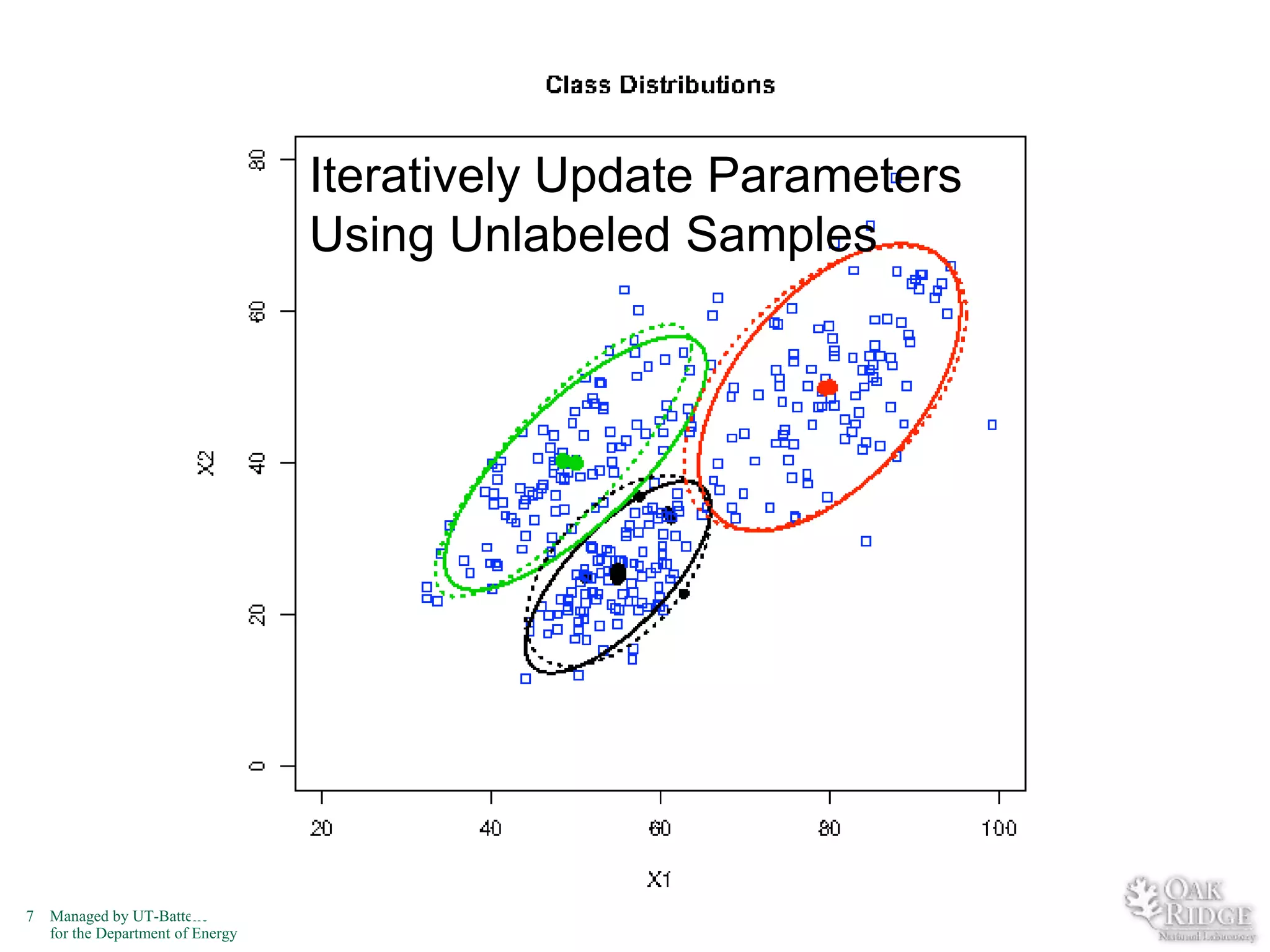
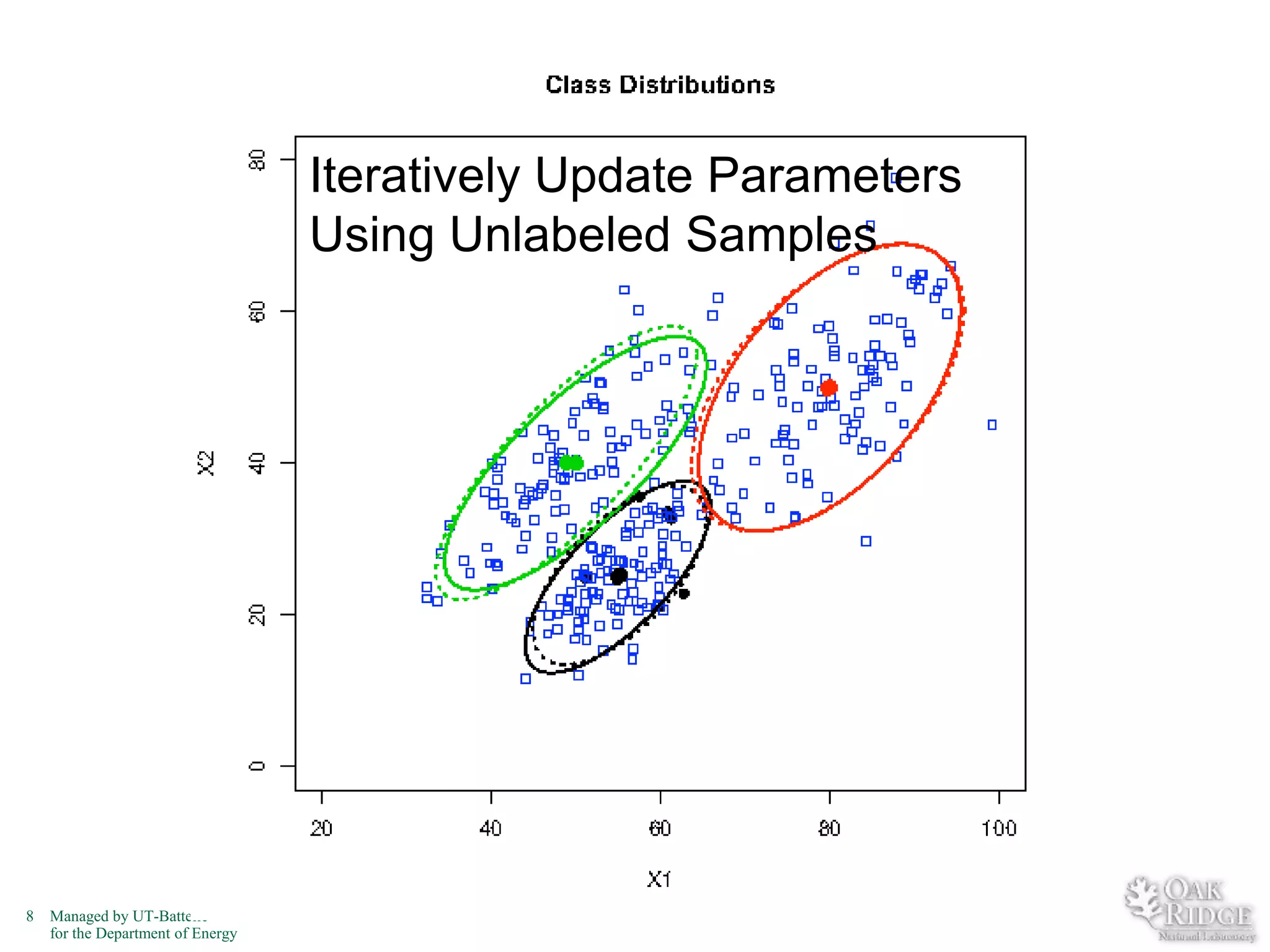
– (Artificially) Increase number of samples
– By incorporating unlabeled samples
Naïve semi-supervised (Nigam et al. [JML-2000])
– Bagging [Breiman, ML-96]
3
Managed by UT-Battelle
for the Department of Energy

4. True Distribution
Estimated Distribution
(Small Samples; MLE
are good asymptotically)
4
Managed by UT-Battelle
for the Department of Energy

5. Initial Estimates +
Unlabeled Samples
5
Managed by UT-Battelle
for the Department of Energy

6. Iteratively Update Parameters
Using Unlabeled Samples
6
Managed by UT-Battelle
for the Department of Energy

7. Iteratively Update Parameters
Using Unlabeled Samples
7
Managed by UT-Battelle
for the Department of Energy

8. Iteratively Update Parameters
Using Unlabeled Samples
8
Managed by UT-Battelle
for the Department of Energy

9. Final parameters
after convergence
9
Managed by UT-Battelle
for the Department of Energy

10. Solution: Semi-supervised Learning
Assume Samples are generated by a
Gaussian Mixture Model (GMM)
• Estimate Parameters with
Expectation Maximization (EM)
E-Step
{
}
T
1
ˆj ˆ j
ˆj
xi - m k ) S-1,k ( xi - m k )
(
2
eij =
-1/2
T
M
1
ˆ
ˆ
ˆ
ˆ
Slk
exp - ( xi - mlk ) S-1,k ( xi - mlk )
ål=1
l
2
ˆ
Skj
-1/2
exp -
{
M-Step
aj
å
=
N
i=1
N
eij
N
ˆj
m k+1
,
i=1 ij i
N
i=1 ij
å
ˆ
Sk+1 = i=1
j
N
and
å ex,
=
å e
ˆj
ˆj
eij ( xi - m k+1 ) ( xi - m k+1 )
å
N
e
i=1 ij
ithdata vector, jth class
10 Managed by UT-Battelle
for the Department of Energy
T
}

11. Results
Small Subset of 20
Training Samples
10 Classes, 100 Training Samples
(10-30) x No of dimensions / class
20 labeled + 80
unlabeled samples
S u p e rvise d (B C ) vs. S e m i-su p e rvise d (B C -E M )
80
Ranga Raju Vatsavai, Shashi Shekhar, Thomas E. Burk: A SemiSupervised Learning Method for Remote Sensing Data Mining.
ICTAI 2005: 207-211
A c c u ra c y
70
60
50
B C - W o rs t
B C - B est
B C (E M ) - B e s t
40
30
0
20
40
60
80
100
F ixe d U n la b e le d (8 5 ) a n d V a ryin g (In c re a s in g ) L a b e le d
11 Managed by UT-Battelle
for the Department of Energy
120

12. Challenge 2: Spatial Homogeneity
Spatial Homogeneity
Bayes Theorem: p(c|x) = p(x|c)p(c)/p(x)
For Markov random field , the conditional
distribution of a point in the field given all other Prior Distribution Model:
points is only dependent on its neighbors.
p{ ( s ) |
Where
(S
s )}
p{ ( s ) |
( s )}
For a first - order neighborhood system
S is an image lattice
S
s denotes a set of points in S excluding s
p( )
1
z
c
t (
e
C
)
e.q.1
c
x
x s x
x
12 Managed by UT-Battelle
for the Department of Energy
x x x
x s x
x x x
x
x x x
x x s x x
x x x
x
t ( ) is the total number of horizantally
and vertially neighboring points of different
value in
in clique c .
e.q.1 is Gibbs distribution and therefore,
an MRF.
is emphirically determined weight.
c
t ( )
1 if
( i, j )
otherwise.
{ 0,
( k ,l )

13. Solution: Spatial Classification
•
•
BC (60%)
BC-EM (68%)
BC-MRF (65%)
BC-EM-MRF (72%)
•
13 Managed by UT-Battelle
for the Department of Energy
Shashi Shekhar, Paul R.
Schrater, Ranga Raju Vatsavai,
Weili Wu, Sanjay Chawla:
Spatial contextual classification
and prediction models for mining
geospatial data. IEEE
Transactions on Multimedia 4(2):
174-188 (2002)
Baris M. Kazar, Shashi Shekhar,
David J. Lilja, Ranga Raju
Vatsavai, R. Kelley Pace:
Comparing Exact and
Approximate Spatial Autoregression Model Solutions for
Spatial Data Analysis. GIScience
2004: 140-161
Ranga Raju Vatsavai, Shashi
Shekhar, Thomas E. Burk: An
efficient spatial semi-supervised
learning algorithm. IJPEDS
22(6): 427-437 (2007)

14. Challenge 3: Spatial Heterogeneity
Going From Local to Global
– Signature continuity is a problem in classifying large
geographic regions
Solutions
– Assume constant variance structure over space, that is, train
one model, use it on other regions – poor performance
– Train separate model for each region – needs lot of data
– Train one model covering samples from all regions – needs
an adaptive model to capture spatial heterogeneity
14 Managed by UT-Battelle
for the Department of Energy

15. Solution: Gaussian Process (GP)
Classification
Change of distribution over space is modeled by
p(x | y) ~ N ( ,
)
p ( x ( s ) | y ) ~ N ( ( s ),
( s ))
Goo Jun, Ranga Raju Vatsavai, Joydeep Ghosh: Spatially Adaptive Classification and Active
Learning of Multispectral Data with Gaussian Processes. SSTDM 2009: 597-603
15 Managed by UT-Battelle
for the Department of Energy

16. Challenge 4: Aggregate Vs. Subclasses
Spectral Classes vs. Thematic Classes
Insufficient Ground-truth
Subjective/domain-dependent
Parametric – assumption violations
16 Managed by UT-Battelle
for the Department of Energy

17. Solution: Sub-class Classification
Coarse-to-fine Resolution Information Extraction
– Characterizing the nature of the change
Fallow to Switch grass, Wheat to Corn, or crop damage
Coarse Classes (MODIS)
Each class is Gaussian
Sub-Classes (AWiFS)
Each class is MoG
Model Selection (BIC,AIC)
How many components?
Parameter Estimation
Semi-supervised Learning
Characterize Changes
17 Managed by UT-Battelle
for the Department of Energy

18. Results: Sub-class
Classification
Dataset:
LandSat ETM+ Data (Cloquet, Carleton,
MN, May 31, 2000)
1.
•6 Bands, 4 Classes, 60 plots
•Independent test data: 205 plots
•Forest (4 Subclasses; 2 subclasses are
combined into 1)
2.
•2 Labeled plots per sub-class
18 Managed by UT-Battelle
for the Department of Energy
Ranga Raju Vatsavai, Shashi Shekhar,
Budhendra L. Bhaduri: A Learning Scheme for
Recognizing Sub-classes from Model Trained on
Aggregate Classes. SSPR/SPR 2008: 967-976
Ranga Raju Vatsavai, Shashi Shekhar,
Budhendra L. Bhaduri: A Semi-supervised
Learning Algorithm for Recognizing Sub-classes.
SSTDM 2008: 458-467

19. Crop (Opium) Classification
Helmand accounts for 75% of the world’s opium
production
GeoEye 4-Band Image, 13th May 2011
19 Managed by UT-Battelle
for the Department of Energy

20. Ground-truth (Aggregate Classes)
Ground-truth collected for 4 classes
1-Other Crops (Yellow), 2-Poppy (Red), 3-Soils
(Cyan), 4-Water (Blue)
20 Managed by UT-Battelle
for the Department of Energy

21. Classified (Aggregate) Image
Maximum Likelihood Classification (Widely used)
Also did lot of other standard classification schemes
– Decision Trees, Random Forest, Neural Nets, …
21 Managed by UT-Battelle
for the Department of Energy

22. Classified (Sub-classes) Image
Sub-class classification – Identifying finer classes from
aggregate class – new scheme
– 1 -> 11,12,13; 2 -> 21,22,23, 3->31,32, 4->41
(Overall Accuracy Improved by ~10%)
22 Managed by UT-Battelle
for the Department of Energy

23. Challenge 5: Phenology
AWiFS (May 3, 2008;
FCC (4,3,2))
23 Managed by UT-Battelle
for the Department of Energy
AWiFS (July 14, 2008;
FCC (4,3,2))
Thematic Classes: C-Corn, S-Soy

24. More Formally
24 Managed by UT-Battelle
for the Department of Energy

25. Solution: Multi-view
Learning
Multi-temporal images are different
views of same phenomena
– Learn single classifier on different views, chose
the best one through empirical evaluation
– Combine different views into a single view, train
classifier on single combined view – stacked
vector approach
– Learn classifier on single view and combine
predictions of individual classifiers – multiple
classifier systems
Bayesian Model Averaging
– Co-training
Learn a classifier independently on each view
Use predictions of each classifier on unlabeled
data instances to augment training dataset for
other classifier
Varun Chandola, Ranga Raju Vatsavai: Multi-temporal remote sensing
image classification - A multi-view approach. CIDU 2010: 258-270
25 Managed by UT-Battelle
for the Department of Energy

26. Conclusions
We developed several innovative solutions that
address big spatiotemporal data challenges
–
–
–
–
Semi-supervised learning
Spatial classification (homogeneity and heterogeneity)
Temporal classification
Sub-class classification
Ongoing
– Transfer learning: Adopt model learned in area to the
other with very little additional ground-truth
– Compound object classification (multiple instance
learning)
– Semantic classification (beyond pixels and objects)
– Scaling
Heterogeneous (OpenMP + MPI + CUDA)
Cloud computing (MapReduce)
26 Managed by UT-Battelle
for the Department of Energy

27. Acknowledgements
Prepared by Oak Ridge National Laboratory,
P.O. Box 2008, Oak Ridge, Tennessee 378316285, managed by UT-Battelle, LLC for the U. S.
Department of Energy under contract no.
DEAC05-00OR22725.
Collaborators and Sponsors
27 Managed by UT-Battelle
for the Department of Energy