SlideShare a Scribd company logo
1 of 84
Download to read offline
263
4.1 Graphing Linear
Inequalities
4.2 Solving Linear
Programming
Problems Graphically
4.3 The Simplex Method:
Solving Standard
Maximization
Problems
4.4 The Simplex Method:
Solving General
Linear Programming
Problems
4.5 The Simplex Method
and Duality
KEY CONCEPTS
REVIEW EXERCISES
CASE STUDY
TECHNOLOGY GUIDES
Linear Programming
4
Web Site
www.FiniteMath.org
At the Web site you will find:
• Section by section tutorials
• A detailed chapter summary
• A true/false quiz
• Additional review exercises
• A linear programming
grapher
• A pivot and Gauss-Jordan
tool
• A simplex method tool
Case Study The Diet Problem
The Galaxy Nutrition health-food mega-store chain provides free online nutritional advice
and support to its customers. As Web site technical consultant, you are planning to con-
struct an interactive Web page to assist customers prepare a diet tailored to their nutri-
tional and budgetary requirements. Ideally, the customer would select foods to consider
and specify nutritional and/or budgetary constraints, and the tool should return the optimal
diet meeting those requirements. You would also like the Web page to allow the customer
to decide whether, for instance, to find the cheapest possible diet meeting the require-
ments, the diet with the lowest number of calories, or the diet with the least total carbohy-
drates. How do you go about constructing such a Web page?
Image
Studios/UpperCut
Images/Getty
Images
Introduction
In this chapter we begin to look at one of the most important types of problems for busi-
ness and the sciences: finding the largest or smallest possible value of some quantity
(such as profit or cost) under certain constraints (such as limited resources). We call such
problems optimization problems because we are trying to find the best, or optimum,
value. The optimization problems we look at in this chapter involve linear functions only
and are known as linear programming (LP) problems. One of the main purposes of cal-
culus, which you may study later, is to solve nonlinear optimization problems.
Linear programming problems involving only two unknowns can usually be solved
by a graphical method that we discuss in Sections 4.1 and 4.2. When there are three or
more unknowns, we must use an algebraic method, as we had to do for systems of linear
equations. The method we use is called the simplex method. Invented in 1947 by
George B. Dantzig✱
(1914–2005), the simplex method is still the most commonly used
technique to solve LP problems in real applications, from finance to the computation of
trajectories for guided missiles.
The simplex method can be used for hand calculations when the numbers are fairly
small and the unknowns are few. Practical problems often involve large numbers and
many unknowns, however. Problems such as routing telephone calls or airplane flights,
or allocating resources in a manufacturing process can involve tens of thousands of un-
knowns. Solving such problems by hand is obviously impractical, and so computers are
regularly used. Although computer programs most often use the simplex method, math-
ematicians are always seeking faster methods. The first radically different method of
solving LP problems was the ellipsoid algorithm published in 1979 by the Soviet math-
ematician Leonid G. Khachiyan2
(1952–2005). In 1984, Narendra Karmarkar (1957–),
a researcher at Bell Labs, created a more efficient method now known as Karmarkar’s
algorithm. Although these methods (and others since developed) can be shown to be
faster than the simplex method in the worst cases, it seems to be true that the simplex
method is still the fastest in the applications that arise in practice.
Calculators and spreadsheets are very useful aids in the simplex method. In prac-
tice, software packages do most of the work, so you can think of what we teach you here
as a peek inside a “black box.” What the software cannot do for you is convert a real sit-
uation into a mathematical problem, so the most important lessons to get out of this
chapter are (1) how to recognize and set up a linear programming problem, and (2) how
to interpret the results.
264 Chapter 4 Linear Programming
Graphing Linear Inequalities
By the end of the next section, we will be solving linear programming (LP) problems
with two unknowns. We use inequalities to describe the constraints in a problem, such as
limitations on resources. Recall the basic notation for inequalities.
4.1
✱ NOTE Dantzig is the real-life
source of the story of the
student who, walking in late
to a math class, copies down
two problems on the board,
thinking they’re homework.
After much hard work he
hands in the solutions, only
to discover that he’s just
solved two famous unsolved
problems. This actually
happened to Dantzig in
graduate school in 1939.1
1
Sources: D. J. Albers and C. Reid, “An Interview of George B. Dantzig: The Father of Linear Programming,”
College Math. Journal, v. 17 (1986), pp. 293–314. Quoted and discussed in the context of the urban legends
it inspired at www.snopes.com/college/homework/unsolvable.asp.
2
Dantzig and Khachiyan died approximately two weeks apart in 2005. The New York Times ran their
obituaries together on May 23, 2005.
Here are the particular kinds of inequalities in which we’re interested:
4.1 Graphing Linear Inequalities 265
Linear Inequalities and Solving Inequalities
An inequality in the unknown x is the statement that one expression involving x
is less than or equal to (or greater than or equal to) another. Similarly, we
can have an inequality in x and y, which involves expressions that contain x and
y; an inequality in x, y, and z; and so on. A linear inequality in one or more
unknowns is an inequality of the form
ax ≤ b (or ax ≥ b), a and b real constants
ax + by ≤ c (or ax + by ≥ c), a, b, and c real constants
ax + by + cz ≤ d, a, b, c, and d real constants
ax + by + cz + dw ≤ e, a, b, c, d, and e real constants
and so on.
Nonstrict Inequalities
a ≤ b means that a is less than or equal to b.
a ≥ b means that a is greater than or equal to b.
Quick Examples
3 ≤ 99, −2 ≤ −2, 0 ≤ 3
3 ≥ 3, 1.78 ≥ 1.76,
1
3
≥
1
4
Rules for Manipulating Inequalities
1. The same quantity can be added to or x ≤ y implies x − 4 ≤ y − 4
subtracted from both sides of an inequality:
If x ≤ y, then x + a ≤ y + a for any real
number a.
2. Both sides of an inequality can be multiplied x ≤ y implies 3x ≤ 3y
or divided by a positive constant:
If x ≤ y and a is positive, then ax ≤ ay.
3. Both sides of an inequality can be multiplied x ≤ y implies −3x ≥ −3y
or divided by a negative constant if the
inequality is reversed:
If x ≤ y and a is negative, then ax ≥ ay.
4. The left and right sides of an inequality can 3x ≥ 5y implies 5y ≤ 3x
be switched if the inequality is reversed:
If x ≤ y, then y ≥ x; if y ≥ x, then x ≤ y.
There are also the inequalities < and >, called strict inequalities because they do not
permit equality. We do not use them in this chapter.
Following are some of the basic rules for manipulating inequalities. Although we
illustrate all of them with the inequality ≤, they apply equally well to inequalities with
≥ and to the strict inequalities < and >.
Quick Examples
Solving Linear Inequalities in Two Variables
Our first goal is to solve linear inequalities in two variables—that is, inequalities of the
form ax + by ≤ c. As an example, let’s solve
2x + 3y ≤ 6.
We already know how to solve the equation 2x + 3y = 6. As we saw in Chapter 1, the
solution of this equation may be pictured as the set of all points (x, y) on the straight-line
graph of the equation. This straight line has x-intercept 3 (obtained by putting y = 0 in
the equation) and y-intercept 2 (obtained by putting x = 0 in the equation) and is shown
in Figure 1.
Notice that, if (x, y) is any point on the line, then x and y not only satisfy the equa-
tion 2x + 3y = 6, but they also satisfy the inequality 2x + 3y ≤ 6, because being equal
to 6 qualifies as being less than or equal to 6.
Do the points on the line give all possible solutions to the inequality?
No. For example, try the origin, (0, 0). Because 2(0) + 3(0) = 0 ≤ 6, the point (0, 0) is
a solution that does not lie on the line. In fact, here is a possibly surprising fact: The so-
lution to any linear inequality in two unknowns is represented by an entire half plane: the
set of all points on one side of the line (including the line itself). Thus, because (0, 0) is
a solution of 2x + 3y ≤ 6 and is not on the line, every point on the same side of the line
as (0, 0) is a solution as well (the colored region below the line in Figure 2 shows which
half plane constitutes the solution set).
To see why the solution set of 2x + 3y ≤ 6 is the entire half plane shown, start with
any point P on the line 2x + 3y = 6. We already know that P is a solution of
2x + 3y ≤ 6. If we choose any point Q directly below P, the x-coordinate of Q will be
the same as that of P, and the y-coordinate will be smaller. So the value of 2x + 3y at Q
will be smaller than the value at P, which is 6. Thus, 2x + 3y < 6 at Q, and so Q is an-
other solution of the inequality. (See Figure 3.) In other words, every point beneath the
line is a solution of 2x + 3y ≤ 6.
On the other hand, any point above the line is directly above a point on the line, and
so 2x + 3y > 6 for such a point. Thus, no point above the line is a solution of
2x + 3y ≤ 6.
266 Chapter 4 Linear Programming
A solution of an inequality in the unknown x is a value for x that makes the inequal-
ity true. For example, 2x + 8 ≥ 89 has a solution x = 50 because 2(50) + 8 ≥ 89.
Of course, it has many other solutions as well. Similarly, a solution of an inequality
in x and y is a pair of values (x, y) making the inequality true. For example, (5, 1) is a
solution of 3x − 2y ≥ 8 because 3(5) − 2(1) ≥ 8. To solve an inequality is to find
the set of all solutions.
Quick Examples
2x + 8 ≥ 89+ Linear inequality in x
2x3
≤ x3
+ y Nonlinear inequality in x and y
3x − 2y ≥ 8 Linear inequality in x and y
x2
+ y2
≤ 19z Nonlinear inequality in x, y, and z
3x − 2y + 4z ≤ 0 Linear inequality in x, y, and z
Figure 1
x
y
2x ⫹ 3y ⫽ 6
Figure 2
x
y
2x ⫹ 3y ⫽ 6
(0, 0)
Solution Set
Figure 3
x
y
2x ⫹ 3y ⫽ 6
2x ⫹ 3y ⬍ 6
Q
P(x, y)
The same kind of argument can be used to show that the solution set of every in-
equality of the form ax + by ≤ c or ax + by ≥ c consists of the half plane above or
below the line ax + by = c. The “test-point” procedure we describe below gives us an
easy method for deciding whether the solution set includes the region above or below
the corresponding line.
Now we are going to do something that will appear backward at first (but makes it
simpler to sketch sets of solutions of systems of linear inequalities). For our standard
drawing of the region of solutions of 2x + 3y ≤ 6, we are going to shade only the part
that we do not want and leave the solution region blank. Think of covering over or
“blocking out” the unwanted points, leaving those that we do want in full view (but re-
member that the points on the boundary line are also points that we want). The result is
Figure 4. The reason we do this should become clear in Example 2.
4.1 Graphing Linear Inequalities 267
Figure 4
x
y
(0, 0)
Solution Set
2x ⫹ 3y ⫽ 6
Sketching the Region Represented by a Linear Inequality
in Two Variables
1. Sketch the straight line obtained by replacing the given inequality with an
equality.
2. Choose a test point not on the line; (0, 0) is a good choice if the line does not
pass through the origin.
3. If the test point satisfies the inequality, then the set of solutions is the entire
region on the same side of the line as the test point. Otherwise, it is the region
on the other side of the line. In either case, shade (block out) the side that does
not contain the solutions, leaving the solution set unshaded.
Quick Example
Here are the three steps used to graph the inequality x + 2y ≥ 5.
x
Solution Set
y
x ⫹ 2y ⫽ 5
x
y
x ⫹ 2y ⫽ 5
Test Point
(0, 0)
x
y
x ⫹ 2y ⫽ 5
1. Sketch the line
x + 2y = 5.
2. Test the point (0, 0)
0 + 2(0)  5
Inequality is not
satisfied.
3. Because the inequality
is not satisfied, shade
the region containing
the test point.
EXAMPLE 1 Graphing Single Inequalities
Sketch the regions determined by each of the following inequalities:
a. 3x − 2y ≤ 6 b. 6x ≤ 12 + 4y c. x ≤ −1 d. y ≥ 0 e. x ≥ 3y
c. The region x ≤ −1 has as boundary the vertical line x = −1. The test point (0, 0) is
not in the solution set, as shown in Figure 6.
d. The region y ≥ 0 has as boundary the horizontal line y = 0 (that is, the x-axis). We
cannot use (0, 0) for the test point because it lies on the boundary line. Instead, we
choose a convenient point not on the line y = 0—say, (0, 1). Because 1 ≥ 0, this
point is in the solution set, giving us the region shown in Figure 7.
e. The line x ≥ 3y has as boundary the line x = 3y or, solving for y,
y =
1
3
x.
This line passes through the origin with slope 1/3, so again we cannot choose the ori-
gin as a test point. Instead, we choose (0, 1). Substituting these coordinates in x ≥ 3y
gives 0 ≥ 3(1), which is false, so (0, 1) is not in the solution set, as shown in Figure 8.
268 Chapter 4 Linear Programming
using Technology
Technology can be used to
graph inequalities. Here is an
outline (see the Technology
Guides at the end of the
chapter for additional details
on using a TI-83/84 Plus or
Excel):
TI-83/84 Plus
Solve the inequality for y and
enter the resulting function of
x; for example,
Y1=-(2/3)*X+2.
Position the cursor on the icon
to the left of Y1 and press
until you see the kind
of shading desired (above or
below the line).
[More details on page 343.]
Excel
Solve the inequality for y and
create a scattergraph using
two points on the line. Then
use the drawing palette to
create a polygon to provide
the shading.
[More details on page 345.]
Web Site
www.FiniteMath.org
 Online Utilities
 Linear Programming
Grapher
Type “graph” and enter one or
more inequalities (each one on
a new line) as shown:
Adjust the graph window set-
tings, and click “Graph.”
ENTER
Solution
a. The boundary line 3x − 2y = 6 has x-intercept 2 and y-intercept −3 (Figure 5).
We use (0, 0) as a test point (because it is not on the line). Because 3(0) − 2(0) ≤ 6,
the inequality is satisfied by the test point (0, 0), and so it lies inside the solution set.
The solution set is shown in Figure 5.
b. The given inequality, 6x ≤ 12 + 4y, can be rewritten in the form ax + by ≤ c by
subtracting 4y from both sides:
6x − 4y ≤ 12.
Dividing both sides by 2 gives the inequality 3x − 2y ≤ 6, which we considered in
part (a). Now, applying the rules for manipulating inequalities does not affect the set
of solutions. Thus, the inequality 6x ≤ 12 + 4y has the same set of solutions as
3x − 2y ≤ 6. (See Figure 5.)
Figure 5
x
y
3x ⫺ 2y ⫽ 6
(0, 0)
Solution Set
Figure 6
x
y
x ⫽ ⫺1
Solution
Set
(0, 0)
Figure 7
x
y
Solution Set
(0, 1)
0
y ⫽ 0
Figure 8
x
y
Solution Set
(0, 1)
1
3
y ⫽ x
4.1 Graphing Linear Inequalities 269
EXAMPLE 2 Graphing Simultaneous Inequalities
Sketch the region of points that satisfy both inequalities:
2x − 5y ≤ 10
x + 2y ≤ 8.
Solution Each inequality has a solution set that is a half plane. If a point is to satisfy
both inequalities, it must lie in both sets of solutions. Put another way, if we cover the
points that are not solutions to 2x − 5y ≤ 10 and then also cover the points that are not
solutions to x + 2y ≤ 8, the points that remain uncovered must be the points we want,
those that are solutions to both inequalities. The result is shown in Figure 9, where the
unshaded region is the set of solutions.✱
As a check, we can look at points in various regions in Figure 9. For example, our
graph shows that (0, 0) should satisfy both inequalities, and it does;
2(0) − 5(0) = 0 ≤ 10
0 + 2(0) = 0 ≤ 8.
On the other hand, (0, 5) should fail to satisfy one of the inequalities.
2(0) − 5(5) = −25 ≤ 10
0 + 2(5) = 10  8
One more: (5, −1) should fail one of the inequalities:
2(5) − 5(−1) = 15  10
5 + 2(−1) = 3 ≤ 8.
Figure 9
Solution
Set
x
y
2x ⫺ 5y ⫽ 10
x ⫹ 2y ⫽ 8
Figure 10
x
y
3x⫺ 2y⫽ 6
x ⫹ y ⫽ ⫺5
y ⫽ 4
A B
C
4
2
⫺5
⫺5
✔
✔
✔
✗
✗
✔
✱ TECHNOLOGY NOTE
Although these graphs are
quite easy to do by hand, the
more lines we have to graph
the more difficult it becomes
to get everything in the right
place, and this is where
graphing technology can
become important. This is
especially true when, for
instance, three or more lines
intersect in points that are
very close together and hard
to distinguish in hand-drawn
graphs.
EXAMPLE 3 Corner Points
Sketch the region of solutions of the following system of inequalities and list the coor-
dinates of all the corner points.
3x − 2y ≤ 6
x + y ≥ −5
y ≤ 4
Solution Shading the regions that we do not want leaves us with the triangle shown in
Figure 10. We label the corner points A, B, and C as shown.
Each of these corner points lies at the intersection of two of the bounding lines. So,
to find the coordinates of each corner point, we need to solve the system of equations
given by the two lines. To do this systematically, we make the following table:
Point Lines through Point Coordinates
A y = 4 (−9, 4)
x + y = −5
B y = 4

14
3
, 4

3x − 2y = 6
C x + y = −5

−
4
5
, −
21
5

3x − 2y = 6
Take another look at the regions of solutions in Examples 2 and 3 (Figure 11).
270 Chapter 4 Linear Programming
✱ TECHNOLOGY NOTE
Using the trace feature makes
it easy to locate corner points
graphically. Remember to
zoom in for additional
accuracy when appropriate.
Of course, you can also use
technology to help solve the
systems of equations, as we
discussed in Chapter 2.
Here, we have solved each system of equations in the middle column to get the point on
the right, using the techniques of Chapter 2. You should do this for practice.✱
As a partial check that we have drawn the correct region, let us choose any point in its
interior—say, (0, 0). We can easily check that (0, 0) satisfies all three given inequalities. It
follows that all of the points in the triangular region containing (0, 0) are also solutions.
Figure 11
Solution
Set
x
y
x
y
Solution Set
(a) Example 2 Solution Set (b) Example 3 Solution Set
Notice that the solution set in Figure 11(a) extends infinitely far to the left, whereas
the one in Figure 11(b) is completely enclosed by a boundary. Sets that are completely
enclosed are called bounded, and sets that extend infinitely in one or more directions
are unbounded. For example, all the solution sets in Example 1 are unbounded.
EXAMPLE 4 Resource Allocation
Socaccio Pistachio Inc. makes two types of pistachio nuts: Dazzling Red and Organic.
Pistachio nuts require food color and salt, and the following table shows the amount of
food color and salt required for a 1-kilogram batch of pistachios, as well as the total
amount of these ingredients available each day.
Use a graph to show the possible numbers of batches of each type of pistachio
Socaccio can produce each day. This region (the solution set of a system of inequalities)
is called the feasible region.
Solution As we did in Chapter 2, we start by identifying the unknowns: Let x be the
number of batches of Dazzling Red manufactured per day and let y be the number of
batches of Organic manufactured each day.
Now, because of our experience with systems of linear equations, we are tempted to
say: For food color 2x + y = 20 and for salt, 10x + 20y = 220. However, no one is say-
ing that Socaccio has to use all available ingredients; the company might choose to use
fewer than the total available amounts if this proves more profitable. Thus, 2x + y can
be anything up to a total of 20. In other words,
2x + y ≤ 20.
Similarly,
10x + 20y ≤ 220.
Dazzling Red Organic Total Available
Food Color (g) 2 1 20
Salt (g) 10 20 220
Before we go on... Every point in the feasible region in Example 4 represents a value
for x and a value for y that do not violate any of the company’s restrictions. For example,
the point (5, 6) lies well inside the region, so the company can produce five batches of
Dazzling Red nuts and six batches of Organic without exceeding the limitations on
ingredients [that is, 2(5) + 6 = 16 ≤ 20 and 10(5) + 20(6) = 170 ≤ 220]. The corner
points A, B, C, and D are significant if the company wishes to realize the greatest profit,
as we will see in Section 4.2. We can find the corners as in the following table:
➡
4.1 Graphing Linear Inequalities 271
There are two more restrictions not explicitly mentioned: Neither x nor y can be nega-
tive. (The company cannot produce a negative number of batches of nuts.) Therefore, we
have the additional restrictions
x ≥ 0 y ≥ 0.
These two inequalities tell us that the feasible region (solution set) is restricted to the
first quadrant, because in the other quadrants, either x or y or both x and y are negative.
So instead of shading out all other quadrants, we can simply restrict our drawing to the
first quadrant.
The (bounded) feasible region shown in Figure 12 is a graphical representation of
the limitations the company faces.
Figure 12
x
y
10x ⫹ 20y ⫽ 220
2x ⫹ y ⫽ 20
A
D
C
B
Feasible Region
20
11
10 22
(We have not listed the lines through the first three corners because their coordi-
nates can be read easily from the graph.) Points on the line segment DB represent use
of all the food color (because the segment lies on the line 2x + y = 20), and points on
the line segment C D represent use of all the salt (because the segment lies on the line
10x + 20y = 220). Note that the point D is the only solution that uses all of both
ingredients. 쮿
Point Lines through Point Coordinates
A (0, 0)
B (10, 0)
C (0, 11)
D 2x + y = 20 (6, 8)
10x + 20y = 220
Recognizing Whether to Use a Linear Inequality or a Linear Equation
How do I know whether to model a situation by a linear inequality like 3x + 2y ≤ 10
or by a linear equation like 3x + 2y = 10?
Here are some key phrases to look for: at most, up to, no more than, at least, or more,
exactly. Suppose, for instance, that nuts cost 3¢, bolts cost 2¢, x is the number of
nuts you can buy, and y is the number of bolts you can buy.
• If you have up to 10¢ to spend, then 3x + 2y ≤ 10.
• If you must spend exactly 10¢, then 3x + 2y = 10.
• If you plan to spend at least 10¢, then 3x + 2y ≥ 10.
The use of inequalities to model a situation is often more realistic than the use of
equations; for instance, one cannot always expect to exactly fill all orders, spend the
exact amount of one’s budget, or keep a plant operating at exactly 100% capacity.
272 Chapter 4 Linear Programming
In Exercises 27–32, we suggest you use technology. Graph
the regions corresponding to the inequalities, and find the
coordinates of all corner points (if any) to two decimal places:
27. 2.1x − 4.3y ≥ 9.7 28. −4.3x + 4.6y ≥ 7.1
29. −0.2x + 0.7y ≥ 3.3
1.1x + 3.4y ≥ 0
30. 0.2x + 0.3y ≥ 7.2
2.5x − 6.7y ≤ 0
31. 4.1x − 4.3y ≤ 4.4
7.5x − 4.4y ≤ 5.7
4.3x + 8.5y ≤ 10
32. 2.3x − 2.4y ≤ 2.5
4.0x − 5.1y ≤ 4.4
6.1x + 6.7y ≤ 9.6
APPLICATIONS
33. Resource Allocation You manage an ice cream factory that
makes two flavors: Creamy Vanilla and Continental Mocha.
Into each quart of Creamy Vanilla go 2 eggs and 3 cups of
cream. Into each quart of Continental Mocha go 1 egg and
3 cups of cream. You have in stock 500 eggs and 900 cups of
cream. Draw the feasible region showing the number of quarts
of vanilla and number of quarts of mocha that can be produced.
Find the corner points of the region. HINT [See Example 4.]
34. Resource Allocation Podunk Institute of Technology’s Math
Department offers two courses: Finite Math and Applied Cal-
culus. Each section of Finite Math has 60 students, and each
section of Applied Calculus has 50. The department is al-
lowed to offer a total of up to 110 sections. Furthermore, no
more than 6,000 students want to take a math course. (No stu-
dent will take more than one math course.) Draw the feasible
region that shows the number of sections of each class that
can be offered. Find the corner points of the region. HINT [See
Example 4.]
35. Nutrition Ruff Inc. makes dog food out of chicken and grain.
Chicken has 10 grams of protein and 5 grams of fat per ounce,
and grain has 2 grams of protein and 2 grams of fat per ounce.
A bag of dog food must contain at least 200 grams of protein
and at least 150 grams of fat. Draw the feasible region that
shows the number of ounces of chicken and number of ounces
of grain Ruff can mix into each bag of dog food. Find the cor-
ner points of the region.
36. Purchasing Enormous State University’s Business School is
buying computers. The school has two models to choose
from: the Pomegranate and the iZac. Each Pomegranate
comes with 400 MB of memory and 80 GB of disk space, and
each iZac has 300 MB of memory and 100 GB of disk space.
For reasons related to its accreditation, the school would like
to be able to say that it has a total of at least 48,000 MB of
memory and at least 12,800 GB of disk space. Draw the fea-
sible region that shows the number of each kind of computer
it can buy. Find the corner points of the region.
왔 more advanced ◆ challenging
indicates exercises that should be solved using technology
In Exercises 1–26, sketch the region that corresponds to the
given inequalities, say whether the region is bounded or
unbounded, and find the coordinates of all corner points (if any).
HINT [See Example 1.]
1. 2x + y ≤ 10 2. 4x − y ≤ 12
3. −x − 2y ≤ 8 4. −x + 2y ≥ 4
5. 3x + 2y ≥ 5 6. 2x − 3y ≤ 7
7. x ≤ 3y 8. y ≥ 3x
9.
3x
4
−
y
4
≤ 1 10.
x
3
+
2y
3
≥ 2
11. x ≥ −5 12. y ≤ −4
13. 4x − y ≤ 8
x + 2y ≤ 2
14. 2x + y ≤ 4
x − 2y ≥ 2
HINT [See Examples 2 and 3.] HINT [See Examples 2 and 3.]
15. 3x + 2y ≥ 6
3x − 2y ≤ 6
x ≥ 0
16. 3x + 2y ≤ 6
3x − 2y ≥ 6
−y ≥ 2
17. x + y ≥ 5
x ≤ 10
y ≤ 8
x ≥ 0, y ≥ 0
18. 2x + 4y ≥ 12
x ≤ 5
y ≤ 3
x ≥ 0, y ≥ 0
19. 20x + 10y ≤ 100
10x + 20y ≤ 100
10x + 10y ≤ 60
x ≥ 0, y ≥ 0
20. 30x + 20y ≤ 600
10x + 40y ≤ 400
20x + 30y ≤ 450
x ≥ 0, y ≥ 0
21. 20x + 10y ≥ 100
10x + 20y ≥ 100
10x + 10y ≥ 80
x ≥ 0, y ≥ 0
22. 30x + 20y ≥ 600
10x + 40y ≥ 400
20x + 30y ≥ 600
x ≥ 0, y ≥ 0
23. −3x + 2y ≤ 5
3x − 2y ≤ 6
x ≤ 2y
x ≥ 0, y ≥ 0
24. −3x + 2y ≤ 5
3x − 2y ≥ 6
y ≤ x/2
x ≥ 0, y ≥ 0
25. 2x − y ≥ 0
x − 3y ≤ 0
x ≥ 0, y ≥ 0
26. −x + y ≥ 0
4x − 3y ≥ 0
x ≥ 0, y ≥ 0
4.1 EXERCISES
37. Nutrition Each serving of Gerber Mixed Cereal for Baby
contains 60 calories and 11 grams of carbohydrates, and each
serving of Gerber Mango Tropical Fruit Dessert contains
80 calories and 21 grams of carbohydrates.3
You want to pro-
vide your child with at least 140 calories and at least 32 grams
of carbohydrates. Draw the feasible region that shows the num-
ber of servings of cereal and number of servings of dessert that
you can give your child. Find the corner points of the region.
38. Nutrition Each serving of Gerber Mixed Cereal for Baby
contains 60 calories, 11 grams of carbohydrates, and no vita-
min C. Each serving of Gerber Apple Banana Juice contains
60 calories, 15 grams of carbohydrates, and 120 percent of
the U.S. Recommended Daily Allowance (RDA) of vitamin C
for infants.4
You want to provide your child with at least
120 calories, at least 26 grams of carbohydrates, and at least
50 percent of the U.S. RDA of vitamin C for infants. Draw the
feasible region that shows the number of servings of cereal
and number of servings of juice that you can give your child.
Find the corner points of the region.
39. Municipal Bond Funds The Pimco New York Municipal
Bond Fund (PNF) and the Fidelity Spartan Mass Fund
(FDMMX) are tax-exempt municipal bond funds. In 2003,
the Pimco fund yielded 6% while the Fidelity fund yielded
5%.5
You would like to invest a total of up to $80,000 and earn
at least $4,200 in interest in the coming year (based on the
given yields). Draw the feasible region that shows how much
money you can invest in each fund. Find the corner points of
the region.
40. Municipal Bond Funds In 2003, the Fidelity Spartan Mass
Fund (FDMMX) yielded 5%, and the Fidelity Spartan Florida
Fund (FFLIX) yielded 7%.6
You would like to invest a total of
up to $60,000 and earn at least $3,500 in interest. Draw the
feasible region that shows how much money you can invest in
each fund (based on the given yields). Find the corner points
of the region.
41. 왔 Investments Your portfolio manager has suggested two
high-yielding stocks: Consolidated Edison (ED) and General
Electric (GE). ED shares cost $40 and yield 6% in dividends.
GE shares cost $16 and yield 7.5% in dividends.7
You have up
to $10,000 to invest, and would like to earn at least $600 in div-
idends. Draw the feasible region that shows how many shares in
each company you can buy. Find the corner points of the re-
gion. (Round each coordinate to the nearest whole number.)
42. 왔 Investments Your friend’s portfolio manager has suggested
two energy stocks: Exxon Mobil (XOM) and British Petroleum
(BP). XOM shares cost $80 and yield 2% in dividends. BP
4.1 Graphing Linear Inequalities 273
shares cost $50 and yield 7% in dividends.8
Your friend has
up to $40,000 to invest, and would like to earn at least $1,400
in dividends. Draw the feasible region that shows how many
shares in each company she can buy. Find the corner points
of the region. (Round each coordinate to the nearest whole
number.)
43. 왔 Advertising You are the marketing director for a company
that manufactures bodybuilding supplements and you are
planning to run ads in Sports Illustrated and GQ Magazine.
Based on readership data, you estimate that each one-page ad
in Sports Illustrated will be read by 650,000 people in your
target group, while each one-page ad in GQ will be read by
150,000.9
You would like your ads to be read by at least three
million people in the target group and, to ensure the broadest
possible audience, you would like to place at least three full-
page ads in each magazine. Draw the feasible region that
shows how many pages you can purchase in each magazine.
Find the corner points of the region. (Round each coordinate
to the nearest whole number.)
44. 왔 Advertising You are the marketing director for a company
that manufactures bodybuilding supplements and you are
planning to run ads in Sports Illustrated and Muscle and Fit-
ness. Based on readership data, you estimate that each one-
page ad in Sports Illustrated will be read by 650,000 people
in your target group, while each one-page ad in Muscle and
Fitness will be read by 250,000 people in your target group.10
You would like your ads to be read by at least four million
people in the target group and, to ensure the broadest possible
audience, you would like to place at least three full-page ads
in each magazine during the year. Draw the feasible region
showing how many pages you can purchase in each magazine.
Find the corner points of the region. (Round each coordinate
to the nearest whole number.)
COMMUNICATION AND REASONING EXERCISES
45. Find a system of inequalities whose solution set is unbounded.
46. Find a system of inequalities whose solution set is empty.
47. How would you use linear inequalities to describe the triangle
with corner points (0, 0), (2, 0), and (0, 1)?
48. Explain the advantage of shading the region of points that do
not satisfy the given inequalities. Illustrate with an example.
49. Describe at least one drawback to the method of finding the
corner points of a feasible region by drawing its graph, when
the feasible region arises from real-life constraints.
3
Source: Nutrition information printed on the jar.
4
Ibid.
5
Yields are rounded. Sources: www.pimcofunds.com, www.fidelity.com.
January 18, 2004.
6
Yields are rounded. Source: www.fidelity.com. January 18, 2004.
7
Share prices and yields are approximate (2008). Source: http://finance
.google.com.
8
Ibid.
9
The readership data for Sports Illustrated is based, in part, on the results
of a readership survey taken in March 2000. The readership data for GQ
is fictitious. Source: Mediamark Research Inc./NewYork Times, May 29,
2000, p. C1.
10
The readership data for both magazines are based on the results of a
readership survey taken in March 2000. Source: Mediamark Research
Inc./NewYork Times, May 29, 2000, p. C1.
50. Draw several bounded regions described by linear inequali-
ties. For each region you draw, find the point that gives the
greatest possible value of x + y. What do you notice?
In Exercises 51–54, you are mixing x grams of ingredient A and
y grams of ingredient B. Choose the equation or inequality that
models the given requirement.
51. There should be at least 3 more grams of ingredient A than
ingredient B.
(A) 3x − y ≤ 0 (B) x − 3y ≥ 0
(C) x − y ≥ 3 (D) 3x − y ≥ 0
52. The mixture should contain at least 25% of ingredient A by
weight.
(A) 4x − y ≤ 0 (B) x − 4y ≥ 0
(C) x − y ≥ 4 (D) 3x − y ≥ 0
53. 왔 There should be at least 3 parts (by weight) of ingredient A
to 2 parts of ingredient B.
(A) 3x − 2y ≥ 0 (B) 2x − 3y ≥ 0
(C) 3x + 2y ≥ 0 (D) 2x + 3y ≥ 0
54. 왔 There should be no more of ingredient A (by weight) than
ingredient B.
(A) x − y = 0 (B) x − y ≤ 0
(C) x − y ≥ 0 (D) x + y ≥ y
274 Chapter 4 Linear Programming
55. 왔 You are setting up a system of inequalities in the unknowns
x and y. The inequalities represent constraints faced by Fly-by-
Night Airlines, where x represents the number of first-class
tickets it should issue for a specific flight and y represents the
number of business-class tickets it should issue for that flight.
You find that the feasible region is empty. How do you inter-
pret this?
56. 왔 In the situation described in the preceding exercise, is it
possible instead for the feasible region to be unbounded?
Explain your answer.
57. 왔 Create an interesting scenario that leads to the following
system of inequalities:
20x + 40y ≤ 1,000
30x + 20y ≤ 1,200
x ≥ 0, y ≥ 0.
58. 왔 Create an interesting scenario that leads to the following
system of inequalities:
20x + 40y ≥ 1,000
30x + 20y ≥ 1,200
x ≥ 0, y ≥ 0.
Solving Linear Programming
Problems Graphically
As we saw in Example 4 in Section 4.1, in some scenarios the possibilities are
restricted by a system of linear inequalities. In that example, it would be natural to ask
which of the various possibilities gives the company the largest profit. This is a kind
of problem known as a linear programming problem (commonly referred to as an
LP problem).
4.2
Linear Programming (LP) Problems
A linear programming problem in two unknowns x and y is one in which we are
to find the maximum or minimum value of a linear expression
ax + by
called the objective function, subject to a number of linear constraints of the
form
cx + dy ≤ e or cx + dy ≥ e.
The largest or smallest value of the objective function is called the optimal value,
and a pair of values of x and y that gives the optimal value constitutes an optimal
solution.
The set of points (x, y) satisfying all the constraints is the feasible region for the
problem. Our methods of solving LP problems rely on the following facts:
4.2 Solving Linear Programming Problems Graphically 275
Quick Example
Maximize p = x + y Objective function
subject to x + 2y ≤ 12
2x + y ≤ 12
x ≥ 0, y ≥ 0.

Constraints
See Example 1 for a method of solving this LP problem (that is, finding an
optimal solution and value).
Fundamental Theorem of Linear Programming
• If an LP problem has optimal solutions, then at least one of these solutions
occurs at a corner point of the feasible region.
• Linear programming problems with bounded, nonempty feasible regions always
have optimal solutions.
Let’s see how we can use this to solve an LP problem, and then we’ll discuss why
it’s true.
EXAMPLE 1 Solving an LP Problem
Maximize p = x + y
subject to x + 2y ≤ 12
2x + y ≤ 12
x ≥ 0, y ≥ 0.
Solution We begin by drawing the feasible region for the problem. We do this using
the techniques of Section 4.1, and we get Figure 13.
Each feasible point (point in the feasible region) gives an x and a y satisfying the
constraints. The question now is, which of these points gives the largest value of the ob-
jective function p = x + y? The Fundamental Theorem of Linear Programming tells us
that the largest value must occur at one (or more) of the corners of the feasible region.
In the following table, we list the coordinates of each corner point and we compute the
value of the objective function at each corner.
Figure 13
x
y
x ⫹ 2y ⫽ 12
2x ⫹ y ⫽ 12
12
6
6 12
A
D
C
B
Feasible Region
Corner Point Lines through Point Coordinates p = x + y
A (0, 0) 0
B (6, 0) 6
C (0, 6) 6
D x + 2y = 12 (4, 4) 8
2x + y = 12
Now we simply pick the one that gives the largest value for p, which is D. Therefore, the
optimal value of p is 8, and an optimal solution is (4, 4).
Now we owe you an explanation of why one of the corner points should be an
optimal solution. The question is, which point in the feasible region gives the largest
possible value of p = x + y?
Consider first an easier question: Which points result in a particular value of p? For
example, which points result in p = 2? These would be the points on the line x + y = 2,
which is the line labeled p = 2 in Figure 14.
Now suppose we want to know which points make p = 4: These would be the
points on the line x + y = 4, which is the line labeled p = 4 in Figure 14. Notice that
this line is parallel to but higher than the line p = 2. (If p represented profit in an appli-
cation, we would call these isoprofit lines, or constant-profit lines.) Imagine moving
this line up or down in the picture. As we move the line down, we see smaller values of
p, and as we move it up, we see larger values. Several more of these lines are drawn in
Figure 14. Look, in particular, at the line labeled p = 10. This line does not meet the
feasible region, meaning that no feasible point makes p as large as 10. Starting with
the line p = 2, as we move the line up, increasing p, there will be a last line that meets
the feasible region. In the figure it is clear that this is the line p = 8, and this meets the
feasible region in only one point, which is the corner point D. Therefore, D gives the
greatest value of p of all feasible points.
If we had been asked to maximize some other objective function, such as
p = x + 3y, then the optimal solution might be different. Figure 15 shows some of
the isoprofit lines for this objective function. This time, the last point that is hit as p
increases is C, not D. This tells us that the optimal solution is (0, 6), giving the optimal
value p = 18.
This discussion should convince you that the optimal value in an LP problem will
always occur at one of the corner points. By the way, it is possible for the optimal value
to occur at two corner points and at all points along an edge connecting them. (Do you
see why?) We will see this in Example 3(b).
Here is a summary of the method we have just been using.
276 Chapter 4 Linear Programming
Figure 14
p ⫽ 10
x
y
A
p ⫽ 8
p ⫽ 6
p ⫽ 4
p ⫽ 2
B
D
C
p ⫽ x ⫹ y
Figure 15
x
y
p ⫽ 18
p ⫽ 12
p ⫽ 6
A
D
C
B
p ⫽ x ⫹ 3y
Graphical Method for Solving Linear Programming
Problems in Two Unknowns (Bounded Feasible Regions)
1. Graph the feasible region and check that it is bounded.
2. Compute the coordinates of the corner points.
3. Substitute the coordinates of the corner points into the objective function to
see which gives the maximum (or minimum) value of the objective function.
4. Any such corner point is an optimal solution.
Note If the feasible region is unbounded, this method will work only if there are
optimal solutions; otherwise, it will not work. We will show you a method for
deciding this on page 280. 쮿
APPLICATIONS
EXAMPLE 2 Resource Allocation
Acme Babyfoods mixes two strengths of apple juice. One quart of Beginner’s juice is
made from 30 fluid ounces of water and 2 fluid ounces of apple juice concentrate. One
quart of Advanced juice is made from 20 fluid ounces of water and 12 fluid ounces of
4.2 Solving Linear Programming Problems Graphically 277
Figure 16
x
y
x ⫹ 6y ⫽ 1,800
A
D
C
B
Feasible Region
3x ⫹ 2y ⫽ 3,000
1,500
1,000 1,800
300
concentrate. Every day Acme has available 30,000 fluid ounces of water and 3,600 fluid
ounces of concentrate. Acme makes a profit of 20¢ on each quart of Beginner’s juice and
30¢ on each quart of Advanced juice. How many quarts of each should Acme make each
day to get the largest profit? How would this change if Acme made a profit of 40¢ on
Beginner’s juice and 20¢ on Advanced juice?
Solution Looking at the question that we are asked, we see that our unknown quanti-
ties are
x = number of quarts of Beginner’s juice made each day
y = number of quarts of Advanced juice made each day.
(In this context, x and y are often called the decision variables, because we must decide
what their values should be in order to get the largest profit.) We can write down the data
given in the form of a table (the numbers in the first two columns are amounts per quart
of juice):
Beginner’s, x Advanced, y Available
Water (ounces) 30 20 30,000
Concentrate (ounces) 2 12 3,600
Profit (¢) 20 30
Because nothing in the problem says that Acme must use up all the water or concentrate,
just that it can use no more than what is available, the first two rows of the table give us
two inequalities:
30x + 20y ≤ 30,000
2x + 12y ≤ 3,600.
Dividing the first inequality by 10 and the second by 2 gives
3x + 2y ≤ 3,000
x + 6y ≤ 1,800.
We also have that x ≥ 0 and y ≥ 0 because Acme can’t make a negative amount of
juice. To finish setting up the problem, we are asked to maximize the profit, which is
p = 20x + 30y. Expressed in ¢
This gives us our LP problem:
Maximize p = 20x + 30y
subject to 3x + 2y ≤ 3,000
x + 6y ≤ 1,800
x ≥ 0, y ≥ 0.
The (bounded) feasible region is shown in Figure 16.
The corners and the values of the objective function are listed in the following table:
Point Lines through Point Coordinates p = 20x + 30y
A (0, 0) 0
B (1,000, 0) 20,000
C (0, 300) 9,000
D 3x + 2y = 3,000 (900, 150) 22,500
x + 6y = 1,800
We can see that, in this case, Acme should make 1,000 quarts of Beginner’s juice and no
Advanced juice, for a largest possible profit of 40,000¢, or $400.
278 Chapter 4 Linear Programming
We are seeking to maximize the objective function p, so we look for corner points that
give the maximum value for p. Because the maximum occurs at the point D, we con-
clude that the (only) optimal solution occurs at D. Thus, the company should make 900
quarts of Beginner’s juice and 150 quarts of Advanced juice, for a largest possible profit
of 22,500¢, or $225.
If, instead, the company made a profit of 40¢ on each quart of Beginner’s juice and
20¢ on each quart of Advanced juice, then we would have p = 40x + 20y. This gives
the following table:
Point Lines through Point Coordinates p = 40x + 20y
A (0, 0) 0
B (1,000, 0) 40,000
C (0, 300) 6,000
D 3x + 2y = 3,000 (900, 150) 39,000
x + 6y = 1,800
Before we go on... Notice that, in the first version of the problem in Example 2, the
company used all the water and juice concentrate:
Water: 30(900) + 20(150) = 30,000
Concentrate: 2(900) + 12(150) = 3,600.
In the second version, it used all the water but not all the concentrate:
Water: 30(100) + 20(0) = 30,000
Concentrate: 2(100) + 12(0) = 200  3,600. 쮿
➡
EXAMPLE 3 Investments
The Solid Trust Savings  Loan Company has set aside $25 million for loans to home
buyers. Its policy is to allocate at least $10 million annually for luxury condominiums.
A government housing development grant it receives requires, however, that at least
one-third of its total loans be allocated to low-income housing.
a. Solid Trust’s return on condominiums is 12% and its return on low-income housing is
10%. How much should the company allocate for each type of housing to maximize
its total return?
b. Redo part (a), assuming that the return is 12% on both condominiums and low-
income housing.
Solution
a. We first identify the unknowns: Let x be the annual amount (in millions of dollars)
allocated to luxury condominiums, and let y be the annual amount allocated to low-
income housing.
We now look at the constraints. The first constraint is mentioned in the first sen-
tence: The total the company can invest is $25 million. Thus,
x + y ≤ 25.
Renaud
Visage/age
fotostock/PhotoLibrary
4.2 Solving Linear Programming Problems Graphically 279
(The company is not required to invest all of the $25 million; rather, it can invest up
to $25 million.) Next, the company has allocated at least $10 million to condos.
Rephrasing this in terms of the unknowns, we get
The amount allocated to condos is at least $10 million.
The phrase “is at least” means ≥. Thus, we obtain a second constraint:
x ≥ 10.
The third constraint is that at least one-third of the total financing must be for low-
income housing. Rephrasing this, we say:
The amount allocated to low-income housing is at least one-third of the total.
Because the total investment will be x + y, we get
y ≥
1
3
(x + y).
We put this in the standard form of a linear inequality as follows:
3y ≥ x + y
−x + 2y ≥ 0.
There are no further constraints.
Now, what about the return on these investments? According to the data, the an-
nual return is given by
p = 0.12x + 0.10y.
We want to make this quantity p as large as possible. In other words, we want to
Maximize p = 0.12x + 0.10y
subject to x + y ≤ 25
x ≥ 10
−x + 2y ≥ 0
x ≥ 0, y ≥ 0.
(Do you see why the inequalities x ≥ 0 and y ≥ 0 are slipped in here?) The feasible
region is shown in Figure 17.
We now make a table that gives the return on investment at each corner point:
Multiply both sides by 3.
Subtract x + y from both sides.
From the table, we see that the values of x and y that maximize the return are
x = 50/3 and y = 25/3, which give a total return of $2.833 million. In other words,
the most profitable course of action is to invest $16.667 million in loans for condo-
miniums and $8.333 million in loans for low-income housing, giving a maximum
annual return of $2.833 million.
Point Lines through Point Coordinates p = 0.12x + 0.10y
A (10, 15) 2.7
B (50/3, 25/3) 2.833
C (10, 5) 1.7
x = 10
x + y = 25
x + y = 25
−x + 2y = 0
x = 10
−x + 2y = 0
Figure 17
x
y
⫺x ⫹ 2y ⫽ 0
x ⫹ y ⫽ 25
B
Feasible
Region
A
C
x ⫽ 10
25
10 25
Looking at the table, we see that a curious thing has happened: We get the same max-
imum annual return at both A and B. Thus, we could choose either option to maximize
the annual return. In fact, any point along the line segment AB will yield an annual
return of $3 million. For example, the point (12, 13) lies on the line segment AB and
also yields an annual revenue of $3 million. This happens because the “isoreturn”
lines are parallel to that edge.
280 Chapter 4 Linear Programming
b. The LP problem is the same as for part (a) except for the objective function:
Maximize p = 0.12x + 0.12y
subject to
x + y ≤ 25
x ≥ 10
−x + 2y ≥ 0
x ≥ 0, y ≥ 0.
Here are the values of p at the three corners:
Point Coordinates p = 0.12x + 0.12y
A (10, 15) 3
B (50/3, 25/3) 3
C (10, 5) 1.8
Before we go on... What breakdowns of investments would lead to the lowest return
for parts (a) and (b)? 쮿
The preceding examples all had bounded feasible regions. If the feasible region is
unbounded, then, provided there are optimal solutions, the fundamental theorem of lin-
ear programming guarantees that the above method will work. The following procedure
determines whether or not optimal solutions exist and finds them when they do.
➡
Solving Linear Programming Problems in Two Unknowns
(Unbounded Feasible Regions)
If the feasible region of an LP problem is unbounded, proceed as follows:
1. Draw a rectangle large enough so that all the corner points are inside the
rectangle (and not on its boundary):
Corner points: A, B, C Corner points inside the rectangle
A
B
C
y
x
Unbounded
Feasible
Region
A
B
C
y
x
In the next two examples, we work with unbounded feasible regions.
4.2 Solving Linear Programming Problems Graphically 281
2. Shade the outside of the rectangle so as to define a new bounded feasible
region, and locate the new corner points:
New corner points: D, E, and F
3. Obtain the optimal solutions using this bounded feasible region.
4. If any optimal solutions occur at one of the original corner points (A, B, and
C in the figure), then the LP problem has that corner point as an optimal
solution. Otherwise, the LP problem has no optimal solutions. When the
latter occurs, we say that the objective function is unbounded, because it
can assume arbitrarily large (positive or negative) values.
A
D E
B
C F
y
x
EXAMPLE 4 Cost
You are the manager of a small store that specializes in hats, sunglasses, and other ac-
cessories. You are considering a sales promotion of a new line of hats and sunglasses.
You will offer the sunglasses only to those who purchase two or more hats, so you will
sell at least twice as many hats as pairs of sunglasses. Moreover, your supplier tells you
that, due to seasonal demand, your order of sunglasses cannot exceed 100 pairs. To en-
sure that the sale items fill out the large display you have set aside, you estimate that you
should order at least 210 items in all.
a. Assume that you will lose $3 on every hat and $2 on every pair of sunglasses sold.
Given the constraints above, how many hats and pairs of sunglasses should you order
to lose the least amount of money in the sales promotion?
b. Suppose instead that you lose $1 on every hat sold but make a profit of $5 on every
pair of sunglasses sold. How many hats and pairs of sunglasses should you order to
make the largest profit in the sales promotion?
c. Now suppose that you make a profit of $1 on every hat sold but lose $5 on every pair
of sunglasses sold. How many hats and pairs of sunglasses should you order to make
the largest profit in the sales promotion?
Solution
a. The unknowns are:
x = number of hats you order
y = number of pairs of sunglasses you order.
The corner point that gives the minimum value of the objective function c is B. Be-
cause B is one of the corner points of the original feasible region, we conclude that
our linear programming problem has an optimal solution at B. Thus, the combination
that gives the smallest loss is 140 hats and 70 pairs of sunglasses.
282 Chapter 4 Linear Programming
The objective is to minimize the total loss:
c = 3x + 2y.
Now for the constraints. The requirement that you will sell at least twice as many
hats as sunglasses can be rephrased as:
The number of hats is at least twice the number of pairs of sunglasses,
or
x ≥ 2y
which, in standard form, is
x − 2y ≥ 0.
Next, your order of sunglasses cannot exceed 100 pairs, so
y ≤ 100.
Finally, you would like to sell at least 210 items in all, giving
x + y ≥ 210.
Thus, the LP problem is the following:
Minimize c = 3x + 2y
subject to x − 2y ≥ 0
y ≤ 100
x + y ≥ 210
x ≥ 0, y ≥ 0.
The feasible region is shown in Figure 18. This region is unbounded, so there is
no guarantee that there are any optimal solutions. Following the procedure described
above, we enclose the corner points in a rectangle as shown in Figure 19. (There are
many infinitely many possible rectangles we could have used. We chose one that gives
convenient coordinates for the new corners.)
We now list all the corners of this bounded region along with the corresponding
values of the objective function c:
Figure 18
x
y
x ⫺ 2y ⫽ 0
x ⫹ y ⫽ 210
y ⫽ 100
100
210
210
A
C
B Feasible
Region
Figure 19
100
210
B
x
y
x ⫺ 2y ⫽ 0
x ⫹ y ⫽ 210
y ⫽ 100
A E
C D
210 300
Point Lines through Point Coordinates c = 3x + 2y ($)
A (210, 0) 630
B (140, 70) 560
C (200, 100) 800
D (300, 100) 1,100
E (300, 0) 900
x + y = 210
x − 2y = 0
x − 2y = 0
y = 100
The corner point that gives the maximum value of the objective function p is C. Be-
cause C is one of the corner points of the original feasible region, we conclude that
our LP problem has an optimal solution at C. Thus, the combination that gives the
largest profit ($300) is 200 hats and 100 pairs of sunglasses.
c. The objective function is now p = x − 5y, which is the negative of the objective
function used in part (b). Thus, the table of values of p is the same as in part (b), ex-
cept that it has opposite signs in the p column. This time we find that the maximum
value of p occurs at E. However, E is not a corner point of the original feasible region,
so the LP problem has no optimal solution. Referring to Figure 18, we can make the
objective p as large as we like by choosing a point far to the right in the unbounded
feasible region. Thus, the objective function is unbounded; that is, it is possible to
make an arbitrarily large profit.
4.2 Solving Linear Programming Problems Graphically 283
b. The LP problem is the following:
Maximize p = −x + 5y
subject to x − 2y ≥ 0
y ≤ 100
x + y ≥ 210
x ≥ 0, y ≥ 0.
Because most of the work is already done for us in part (a), all we need to do is change
the objective function in the table that lists the corner points:
Point Lines through Point Coordinates p = −x + 5y ($)
A (210, 0) −210
B (140, 70) 210
C (200, 100) 300
D (300, 100) 200
E (300, 0) −300
x + y = 210
x − 2y = 0
x − 2y = 0
y = 100
EXAMPLE 5 Resource Allocation
You are composing a very avant-garde ballade for violins and bassoons. In your ballade,
each violinist plays a total of two notes and each bassoonist only one note. To make your
ballade long enough, you decide that it should contain at least 200 instrumental notes.
Furthermore, after playing the requisite two notes, each violinist will sing one soprano
note, while each bassoonist will sing three soprano notes.* To make the ballade suffi-
ciently interesting, you have decided on a minimum of 300 soprano notes. To give your
composition a sense of balance, you wish to have no more than three times as many bas-
soonists as violinists. Violinists charge $200 per performance and bassoonists $400 per
performance. How many of each should your ballade call for in order to minimize
personnel costs?
*Whether or not these musicians are capable of singing decent soprano notes will be left to chance. You
reason that a few bad notes will add character to the ballade.
From the table we see that the minimum cost occurs at B, a corner point of the original
feasible region. The linear programming problem thus has an optimal solution, and the
minimum cost is $44,000 per performance, employing 60 violinists and 80 bassoonists.
(Quite a wasteful ballade, one might say.)
284 Chapter 4 Linear Programming
Solution First, the unknowns are x = number of violinists and y = number of bas-
soonists. The constraint on the number of instrumental notes implies that
2x + y ≥ 200
because the total number is to be at least 200. Similarly, the constraint on the number of
soprano notes is
x + 3y ≥ 300.
The next one is a little tricky. As usual, we reword it in terms of the quantities x and y.
The number of bassoonists should be no more than three times the number of violinists.
Thus, y ≤ 3x
or 3x − y ≥ 0.
Finally, the total cost per performance will be
c = 200x + 400y.
We wish to minimize total cost. So, our linear programming problem is as follows:
Minimize c = 200x + 400y
subject to 2x + y ≥ 200
x + 3y ≥ 300
3x − y ≥ 0
x ≥ 0, y ≥ 0.
We get the feasible region shown in Figure 20.✱
The feasible region is unbounded, and
so we add a convenient rectangle as before (Figure 21).
Figure 20
x
y
x ⫹ 3y ⫽ 300
y ⫽ 3x
2x ⫹ y ⫽ 200
A
C
B
200
100
100 300
Feasible Region
Figure 21
x
y
x ⫹ 3y ⫽ 300
y ⫽ 3x
2x ⫹ y ⫽ 200
A
E
C
D
F
B
200
150
100
100 300 400
Point Lines through Point Coordinates c = 200x + 400y
A (40, 120) 56,000
B (60, 80) 44,000
C (300, 0) 60,000
D (50, 150) 70,000
E (400, 150) 140,000
F (400, 0) 80,000
2x + y = 200
3x − y = 0
2x + y = 200
x + 3y = 300
3x − y = 0
y = 150
✱ NOTE In Figure 20 you can
see how graphing technology
would help in determining the
corner points: Unless you are
very confident in the accuracy
of your sketch, how do you
know that the line y = 3x falls
to the left of the point B? If it
were to fall to the right, then B
would not be a corner point
and the solution would be
different. You could (and
should) check that B satisfies
the inequality 3x − y ≥ 0, so
that the line falls to the left of
B as shown. However, if you
use a graphing calculator or
computer, you can be fairly
confident of the picture
produced without doing
further calculations.
4.2 Solving Linear Programming Problems Graphically 285
Recognizing a Linear Programming Problem, Setting Up Inequalities,
and Dealing with Unbounded Regions
How do I recognize when an application leads to an LP problem as opposed to a
system of linear equations?
Here are some cues that suggest an LP problem:
• Key phrases suggesting inequalities rather than equalities, like at most, up to, no
more than, at least, and or more.
• A quantity that is being maximized or minimized (this will be the objective). Key
phrases are maximum, minimum, most, least, largest, greatest, smallest, as large
as possible, and as small as possible.
How do I deal with tricky phrases like “there should be no more than twice as many
nuts as bolts” or “at least 50% of the total should be bolts”?
The easiest way to deal with phrases like this is to use the technique we discussed in
Chapter 2: reword the phrases using “the number of . . . ”, as in
The number of nuts (x) is no more than twice the number of bolts (y) x ≤ 2y
The number of bolts is at least 50% of the total y ≥ 0.50(x + y)
Do I always have to add a rectangle to deal with unbounded regions?
Under some circumstances, you can tell right away whether optimal solutions exist,
even when the feasible region is unbounded.
Note that the following apply only when we have the constraints x ≥ 0 and y ≥ 0.
1. If you are minimizing c = ax + by with a and b non-negative, then optimal solu-
tions always exist. (Examples 4(a) and 5 are of this type.)
2. If you are maximizing p = ax + by with a and b non-negative (and not both zero),
then there is no optimal solution unless the feasible region is bounded.
Do you see why statements (1) and (2) are true?
Web Site
www.FiniteMath.org
For an online utility that does
everything (solves linear
programming problems with
two unknowns and even draws
the feasible region), go to the
Web site and follow
 Online Utilities
 Linear Programming
Grapher.
3. Minimize c = x + y 4. Minimize c = x + 2y
subject to x + 2y ≥ 6
2x + y ≥ 6
x ≥ 0, y ≥ 0.
subject to x + 3y ≥ 30
2x + y ≥ 30
x ≥ 0, y ≥ 0.
5. Maximize p = 3x + y 6. Maximize p = x − 2y
subject to 3x − 7y ≤ 0
7x − 3y ≥ 0
x + y ≤ 10
x ≥ 0, y ≥ 0.
subject to x + 2y ≤ 8
x − 6y ≤ 0
3x − 2y ≥ 0
x ≥ 0, y ≥ 0.
왔 more advanced ◆ challenging
indicates exercises that should be solved using technology
In Exercises 1–20, solve the LP problems. If no optimal solution
exists, indicate whether the feasible region is empty or the objec-
tive function is unbounded. HINT [See Example 1.]
1. Maximize p = x + y 2. Maximize p = x + 2y
subject to x + 2y ≤ 9
2x + y ≤ 9
x ≥ 0, y ≥ 0.
subject to x + 3y ≤ 24
2x + y ≤ 18
x ≥ 0, y ≥ 0.
4.2 EXERCISES
7. Maximize p = 3x + 2y
subject to 0.2x + 0.1y ≤ 1
0.15x + 0.3y ≤ 1.5
10x + 10y ≤ 60
x ≥ 0, y ≥ 0.
8. Maximize p = x + 2y
subject to 30x + 20y ≤ 600
0.1x + 0.4y ≤ 4
0.2x + 0.3y ≤ 4.5
x ≥ 0, y ≥ 0.
9. Minimize c = 0.2x + 0.3y
subject to 0.2x + 0.1y ≥ 1
0.15x + 0.3y ≥ 1.5
10x + 10y ≥ 80
x ≥ 0, y ≥ 0.
10. Minimize c = 0.4x + 0.1y
subject to 30x + 20y ≥ 600
0.1x + 0.4y ≥ 4
0.2x + 0.3y ≥ 4.5
x ≥ 0, y ≥ 0.
11. Maximize and minimize p = x + 2y
subject to x + y ≥ 2
x + y ≤ 10
x − y ≤ 2
x − y ≥ −2.
12. Maximize and minimize p = 2x − y
subject to x + y ≥ 2
x − y ≤ 2
x − y ≥ −2
x ≤ 10, y ≤ 10.
13. Maximize p = 2x + 3y
subject to 0.1x + 0.2y ≥ 1
2x + y ≥ 10
x ≥ 0, y ≥ 0.
14. Maximize p = 3x + 2y
subject to 0.1x + 0.1y ≥ 0.2
y ≤ 10
x ≥ 0, y ≥ 0.
15. Minimize c = 2x + 4y
subject to 0.1x + 0.1y ≥ 1
x + 2y ≥ 14
x ≥ 0, y ≥ 0.
16. Maximize p = 2x + 3y
subject to −x + y ≥ 10
x + 2y ≤ 12
x ≥ 0, y ≥ 0.
17. 왔 Minimize c = 3x − 3y
subject to
x
4
≤ y
y ≤
2x
3
x + y ≥ 5
x + 2y ≤ 10
x ≥ 0, y ≥ 0.
18. 왔 Minimize c = −x + 2y
subject to y ≤
2x
3
x ≤ 3y
y ≥ 4
x ≥ 6
x + y ≤ 16.
19. 왔 Maximize p = x + y
subject to x + 2y ≥ 10
2x + 2y ≤ 10
2x + y ≥ 10
x ≥ 0, y ≥ 0.
20. 왔 Minimize c = 3x + y
subject to 10x + 20y ≥ 100
0.3x + 0.1y ≥ 1
x ≥ 0, y ≥ 0.
APPLICATIONS
21. Resource Allocation You manage an ice cream factory that
makes two flavors: Creamy Vanilla and Continental Mocha.
Into each quart of Creamy Vanilla go 2 eggs and 3 cups of
cream. Into each quart of Continental Mocha go 1 egg and
3 cups of cream. You have in stock 500 eggs and 900 cups of
cream. You make a profit of $3 on each quart of Creamy
Vanilla and $2 on each quart of Continental Mocha. How
many quarts of each flavor should you make in order to earn
the largest profit? HINT [See Example 2.]
22. Resource Allocation Podunk Institute of Technology’s Math
Department offers two courses: Finite Math and Applied Cal-
culus. Each section of Finite Math has 60 students, and each
section of Applied Calculus has 50. The department is
allowed to offer a total of up to 110 sections. Furthermore, no
more than 6,000 students want to take a math course (no stu-
dent will take more than one math course). Suppose the uni-
versity makes a profit of $100,000 on each section of Finite
Math and $50,000 on each section of Applied Calculus (the
286 Chapter 4 Linear Programming
profit is the difference between what the students are charged
and what the professors are paid). How many sections of
each course should the department offer to make the largest
profit? HINT [See Example 2.]
23. Nutrition Ruff, Inc. makes dog food out of chicken and grain.
Chicken has 10 grams of protein and 5 grams of fat per ounce,
and grain has 2 grams of protein and 2 grams of fat per ounce.
A bag of dog food must contain at least 200 grams of protein
and at least 150 grams of fat. If chicken costs 10¢ per ounce
and grain costs 1¢ per ounce, how many ounces of each
should Ruff use in each bag of dog food in order to minimize
cost? HINT [See Example 4.]
24. Purchasing Enormous State University’s Business School is
buying computers. The school has two models from which to
choose, the Pomegranate and the iZac. Each Pomegranate
comes with 400 MB of memory and 80 GB of disk space;
each iZac has 300 MB of memory and 100 GB of disk space.
For reasons related to its accreditation, the school would like
to be able to say that it has a total of at least 48,000 MB of
memory and at least 12,800 GB of disk space. If the Pome-
granate and the iZac cost $2,000 each, how many of each
should the school buy to keep the cost as low as possible? HINT
[See Example 4.]
25. Nutrition Each serving of Gerber Mixed Cereal for Baby con-
tains 60 calories and 11 grams of carbohydrates. Each serving
of Gerber Mango Tropical Fruit Dessert contains 80 calories
and 21 grams of carbohydrates.11
If the cereal costs 30¢ per
serving and the dessert costs 50¢ per serving, and you want
to provide your child with at least 140 calories and at least
32 grams of carbohydrates, how can you do so at the least
cost? (Fractions of servings are permitted.)
26. Nutrition Each serving of Gerber Mixed Cereal for Baby con-
tains 60 calories, 10 grams of carbohydrates, and no vitamin C.
Each serving of Gerber Apple Banana Juice contains 60 calo-
ries, 15 grams of carbohydrates, and 120 percent of the U.S.
Recommended Daily Allowance (RDA) of vitamin C for
infants. The cereal costs 10¢ per serving and the juice costs
30¢ per serving. If you want to provide your child with at
least 120 calories, at least 25 grams of carbohydrates, and at
least 60 percent of the U.S. RDA of vitamin C for infants,
how can you do so at the least cost? (Fractions of servings are
permitted.)
27. Energy EfficiencyYou are thinking of making your home more
energy efficient by replacing some of the light bulbs with com-
pact fluorescent bulbs, and insulating part or all of your exterior
walls. Each compact fluorescent light bulb costs $4 and saves
you an average of $2 per year in energy costs, and each square
foot of wall insulation costs $1 and saves you an average of
$0.20 per year in energy costs.12
Your home has 60 light fittings
and 1,100 sq. ft. of uninsulated exterior wall. You can spend no
more than $1,200 and would like to save as much per year in en-
ergy costs as possible. How many compact fluorescent light
bulbs and how many square feet of insulation should you
purchase? How much will you save in energy costs per year?
28. Energy Efficiency (Compare with the preceding exercise.)
You are thinking of making your mansion more energy effi-
cient by replacing some of the light bulbs with compact fluo-
rescent bulbs, and insulating part or all of your exterior walls.
Each compact fluorescent light bulb costs $4 and saves you an
average of $2 per year in energy costs, and each square foot of
wall insulation costs $1 and saves you an average of $0.20 per
year in energy costs.13
Your mansion has 200 light fittings and
3,000 sq. ft. of uninsulated exterior wall. To impress your
friends, you would like to spend as much as possible, but save
no more than $800 per year in energy costs (you are proud of
your large utility bills). How many compact fluorescent light
bulbs and how many square feet of insulation should you pur-
chase? How much will you save in energy costs per year?
Creatine Supplements Exercises 29 and 30 are based on the
following data on three bodybuilding supplements. (Figures
shown correspond to a single serving.)14
4.2 Solving Linear Programming Problems Graphically 287
11
Source: Nutrition information printed on the containers.
12
Source: American Council for an Energy-Efficient Economy/NewYork
Times, December 1, 2003, p. C6.
13
Ibid.
14
Source: Nutritional information supplied by the manufacturers
(www.netrition.com). Cost per serving is approximate.
Creatine Carbohydrates Taurine Alpha Lipoic Cost
(g) (g) (g) Acid (mg) ($)
Cell-Tech®
10 75 2 200 2.20
(MuscleTech)
RiboForce HP®
5 15 1 0 1.60
(EAS)
Creatine Transport®
5 35 1 100 0.60
(Kaizen)
29. You are thinking of combining Cell-Tech and RiboForce HP
to obtain a 10-day supply that provides at least 80 grams
of creatine and at least 10 grams of taurine, but no more than
750 grams of carbohydrates and no more than 1,000 mil-
ligrams of alpha lipoic acid. How many servings of each sup-
plement should you combine to meet your specifications at
the least cost?
30. You are thinking of combining Cell-Tech and Creatine Trans-
port to obtain a 10-day supply that provides at least 80 grams
of creatine and at least 10 grams of taurine, but no more than
600 grams of carbohydrates and no more than 2,000 mil-
ligrams of alpha lipoic acid. How many servings of each sup-
plement should you combine to meet your specifications at
the least cost?
31. Resource Allocation Your salami manufacturing plant can
order up to 1,000 pounds of pork and 2,400 pounds of beef
per day for use in manufacturing its two specialties: “Count
Dracula Salami” and “Frankenstein Sausage.” Production of
the Count Dracula variety requires 1 pound of pork and
3 pounds of beef for each salami, while the Frankenstein vari-
ety requires 2 pounds of pork and 2 pounds of beef for every
sausage. In view of your heavy investment in advertising
Count Dracula Salami, you have decided that at least one-
third of the total production should be Count Dracula. On the
other hand, due to the health-conscious consumer climate,
your Frankenstein Sausage (sold as having less beef) is earning
your company a profit of $3 per sausage, while sales of the
Count Dracula variety are down and it is earning your com-
pany only $1 per salami. Given these restrictions, how many
of each kind of sausage should you produce to maximize
profits, and what is the maximum possible profit? HINT [See
Example 3.]
32. Project Design The Megabuck Hospital Corp. is to build a
state-subsidized nursing home catering to homeless patients
as well as high-income patients. State regulations require that
every subsidized nursing home must house a minimum of
1,000 homeless patients and no more than 750 high-income
patients in order to qualify for state subsidies. The overall
capacity of the hospital is to be 2,100 patients. The board of
directors, under pressure from a neighborhood group, insists
that the number of homeless patients should not exceed twice
the number of high-income patients. Due to the state subsidy,
the hospital will make an average profit of $10,000 per month
for every homeless patient it houses, whereas the profit per
high-income patient is estimated at $8,000 per month. How
many of each type of patient should it house in order to maxi-
mize profit? HINT [See Example 3.]
33. Television Advertising In February 2008, each episode of
“American Idol” was typically seen by 28.5 million viewers,
while each episode of “Back toYou” was seen by 12.3 million
viewers.15
Your marketing services firm has been hired to
promote Bald No More’s hair replacement process by buying
at least 30 commercial spots during episodes of “American
Idol” and “Back to You.” The cable company running “Amer-
ican Idol” has quoted a price of $3,000 per spot, while the
cable company showing “Back to You” has quoted a price of
$1,000 per spot. Bald No More’s advertising budget for TV
commercials is $120,000, and it would like no more than 50%
of the total number of spots to appear on “Back to You.” How
many spots should you purchase on each show to reach the
most viewers?
34. Television Advertising In February 2002, each episode of
“Boston Public” was typically seen in 7.0 million homes,
while each episode of “NYPD Blue” was seen in 7.8 million
homes.16
Your marketing services firm has been hired to pro-
mote Gauss Jordan Sneakers by buying at least 30 commer-
cial spots during episodes of “Boston Public” and “NYPD
Blue.” The cable company running “Boston Public” has
quoted a price of $2,000 per spot, while the cable company
showing “NYPD Blue” has quoted a price of $3,000 per spot.
Gauss Jordan Sneakers’ advertising budget for TV commer-
cials is $70,000, and it would like at least 75% of the total
number of spots to appear on “Boston Public.” How many
spots should you purchase on each show to reach the most
homes?
Investing Exercises 35 and 36 are based on the following data
on four stocks.17
288 Chapter 4 Linear Programming
15
Ratings are for February 26, 2008. Source: Nielsen Media Research
(www.tvbythenumbers.com).
16
Ratings are for February 18–24, 2002. Source: Nielsen Media
Research (www.ptd.net) February 28, 2002.
17
Approximate trading price in fourth quarter of 2008 based on 50-day
averages. Earnings per share are rounded. Source: http://finance
.google.com.
18
Share prices and yields are approximate (2008). Source: http://finance
.google.com.
19
Ibid.
Earnings
Price DividendYield per Share
ATRI (Atrion) $90 1% $7.50
BBY (Best Buy) 20 2 3.20
IMCL 70 0 −0.70
(ImClone Systems)
TR (Tootsie Roll) 25 1 0.80
35. 왔 You are planning to invest up to $10,000 in ATRI and BBY
shares.You want your investment to yield at least $120 in div-
idends and you want to maximize the total earnings. How
many shares of each company should you purchase?
36. 왔 You are planning to invest up to $43,000 in IMCL and TR
shares. For tax reasons, you want your investment to yield no
more than $10 in dividends. You want to maximize the total
earnings. How many shares of each company should you
purchase?
37. 왔 Investments Your portfolio manager has suggested two
high-yielding stocks: Consolidated Edison (ED) and General
Electric (GE). ED shares cost $40, yield 6% in dividends, and
have a risk index of 2.0 per share. GE shares cost $16, yield
7.5% in dividends, and have a risk index of 3.0 per share.18
You have up to $10,000 to invest, and would like to earn at
least $600 in dividends. How many shares (to the nearest
tenth of a unit) of each stock should you purchase to meet
your requirements and minimize the total risk index for your
portfolio? What is the minimum total risk index?
38. 왔 Investments Your friend’s portfolio manager has suggested
two energy stocks: Exxon Mobil (XOM) and British Petroleum
(BP). XOM shares cost $80, yield 2% in dividends, and have
a risk index of 2.5. BP shares cost $50, yield 7% in dividends,
and have a risk index of 4.5.19
Your friend has up to $40,000
to invest, and would like to earn at least $1,400 in dividends.
How many shares (to the nearest tenth of a unit) of each stock
should she purchase to meet your requirements and minimize
the total risk index for your portfolio? What is the minimum
total risk index?
39. 왔 Planning My friends: I, the mighty Brutus, have decided to
prepare for retirement by instructing young warriors in the
arts of battle and diplomacy. For each hour spent in battle
instruction, I have decided to charge 50 ducats. For each hour
in diplomacy instruction I shall charge 40 ducats. Due to my
advancing years, I can spend no more than 50 hours per week
instructing the youths, although the great Jove knows that
they are sorely in need of instruction! Due to my fondness for
physical pursuits, I have decided to spend no more than one-
third of the total time in diplomatic instruction. However, the
present border crisis with the Gauls is a sore indication of our
poor abilities as diplomats. As a result, I have decided to
spend at least 10 hours per week instructing in diplomacy.
Finally, to complicate things further, there is the matter of
Scarlet Brew: I have estimated that each hour of battle
instruction will require 10 gallons of Scarlet Brew to quench
my students’ thirst, and that each hour of diplomacy instruc-
tion, being less physically demanding, requires half that
amount. Because my harvest of red berries has far exceeded
my expectations, I estimate that I’ll have to use at least
400 gallons per week in order to avoid storing the fine brew at
great expense. Given all these restrictions, how many hours
per week should I spend in each type of instruction to maxi-
mize my income?
40. 왔 Planning Repeat the preceding exercise with the following
changes: I would like to spend no more than half the total time
in diplomatic instruction, and I must use at least 600 gallons
of Scarlet Brew.
41. 왔 Resource Allocation One day, Gillian the magician sum-
moned the wisest of her women. “Devoted followers,” she
began, “I have a quandary: As you well know, I possess great
expertise in sleep spells and shock spells, but unfortunately,
these are proving to be a drain on my aural energy resources;
each sleep spell costs me 500 pico-shirleys of aural energy,
while each shock spell requires 750 pico-shirleys. Clearly, I
would like to hold my overall expenditure of aural energy to
a minimum, and still meet my commitments in protecting
the Sisterhood from the ever-present threat of trolls. Specif-
ically, I have estimated that each sleep spell keeps us safe for
an average of two minutes, while every shock spell protects
us for about three minutes. We certainly require enough pro-
tection to last 24 hours of each day, and possibly more, just
to be safe. At the same time, I have noticed that each of my
sleep spells can immobilize three trolls at once, while one of
my typical shock spells (having a narrower range) can im-
mobilize only two trolls at once. We are faced, my sisters,
with an onslaught of 1,200 trolls per day! Finally, as you are
no doubt aware, the bylaws dictate that for a Magician of the
Order to remain in good standing, the number of shock
spells must be between one-quarter and one-third the num-
ber of shock and sleep spells combined. What do I do, oh
Wise Ones?”
42. 왔 Risk Management The Grand Vizier of the Kingdom of
Um is being blackmailed by numerous individuals and is
having a very difficult time keeping his blackmailers from
going public. He has been keeping them at bay with two
kinds of payoff: gold bars from the Royal Treasury and po-
litical favors. Through bitter experience, he has learned that
each payoff in gold gives him peace for an average of about
1 month, while each political favor seems to earn him about
a month and a half of reprieve. To maintain his flawless rep-
utation in the Court, he feels he cannot afford any revela-
tions about his tainted past to come to light within the next
year. Thus it is imperative that his blackmailers be kept at
bay for 12 months. Furthermore, he would like to keep the
number of gold payoffs at no more than one-quarter of the
combined number of payoffs because the outward flow of
gold bars might arouse suspicion on the part of the Royal
Treasurer. The Grand Vizier feels that he can do no more
than seven political favors per year without arousing undue
suspicion in the Court. The gold payoffs tend to deplete his
travel budget. (The treasury has been subsidizing his numer-
ous trips to the Himalayas.) He estimates that each gold bar
removed from the treasury will cost him four trips. On the
other hand because the administering of political favors
tends to cost him valuable travel time, he suspects that each
political favor will cost him about two trips. Now, he would
obviously like to keep his blackmailers silenced and lose as
few trips as possible. What is he to do? How many trips will
he lose in the next year?
43. ◆ Management20
You are the service manager for a supplier
of closed-circuit television systems. Your company can pro-
vide up to 160 hours per week of technical service for your
customers, although the demand for technical service far ex-
ceeds this amount. As a result, you have been asked to de-
velop a model to allocate service technicians’ time between
new customers (those still covered by service contracts) and
old customers (whose service contracts have expired). To en-
sure that new customers are satisfied with your company’s
service, the sales department has instituted a policy that at
least 100 hours per week be allocated to servicing new cus-
tomers. At the same time, your superiors have informed you
that the company expects your department to generate at least
$1,200 per week in revenues. Technical service time for new
customers generates an average of $10 per hour (because
much of the service is still under warranty) and for old cus-
tomers generates $30 per hour. How many hours per week
should you allocate to each type of customer to generate the
most revenue?
4.2 Solving Linear Programming Problems Graphically 289
20
Loosely based on a similiar problem in An Introduction to Management
Science (6th Ed.) by D. R. Anderson, D. J. Sweeny and T. A. Williams
(West, 1991).
44. ◆ Scheduling21
The Scottsville Textile Mill produces several
different fabrics on eight dobby looms which operate 24 hours
per day and are scheduled for 30 days in the coming month.
The Scottsville Textile Mill will produce only Fabric 1 and
Fabric 2 during the coming month. Each dobby loom can turn
out 4.63 yards of either fabric per hour. Assume that there is a
monthly demand of 16,000 yards of Fabric 1 and 12,000 yards
of Fabric 2. Profits are calculated as 33¢ per yard for each fab-
ric produced on the dobby looms.
a. Will it be possible to satisfy total demand?
b. In the event that total demand is not satisfied, the
Scottsville Textile Mill will need to purchase the fabrics
from another mill to make up the shortfall. Its profits on
resold fabrics ordered from another mill amount to 20¢
per yard for Fabric 1 and 16¢ per yard for Fabric 2. How
many yards of each fabric should it produce to maximize
profits?
COMMUNICATION AND REASONING EXERCISES
45. If a linear programming problem has a bounded, nonempty
feasible region, then optimal solutions
(A) must exist (B) may or may not exist (C) cannot exist
46. If a linear programming problem has an unbounded, non-
empty feasible region, then optimal solutions
(A) must exist (B) may or may not exist (C) cannot exist
47. What can you say if the optimal value occurs at two adjacent
corner points?
48. Describe at least one drawback to using the graphical method
to solve a linear programming problem arising from a real-life
situation.
49. Create a linear programming problem in two variables that
has no optimal solution.
50. Create a linear programming problem in two variables that
has more than one optimal solution.
51. Create an interesting scenario leading to the following linear
programming problem:
Maximize p = 10x + 10y
subject to 20x + 40y ≤ 1,000
30x + 20y ≤ 1,200
x ≥ 0, y ≥ 0.
52. Create an interesting scenario leading to the following linear
programming problem:
Minimize c = 10x + 10y
subject to 20x + 40y ≥ 1,000
30x + 20y ≥ 1,200
x ≥ 0, y ≥ 0.
53. 왔 Use an example to show why there may be no optimal so-
lution to a linear programming problem if the feasible region
is unbounded.
54. 왔 Use an example to illustrate why, in the event that an opti-
mal solution does occur despite an unbounded feasible re-
gion, that solution corresponds to a corner point of the feasi-
ble region.
55. 왔 You are setting up an LP problem for Fly-by-Night Airlines
with the unknowns x and y, where x represents the number of
first-class tickets it should issue for a specific flight and y rep-
resents the number of business-class tickets it should issue for
that flight, and the problem is to maximize profit.You find that
there are two different corner points that maximize the profit.
How do you interpret this?
56. 왔 In the situation described in the preceding exercise, you
find that there are no optimal solutions. How do you interpret
this?
57. ◆ Consider the following example of a nonlinear program-
ming problem: Maximize p = xy subject to x ≥ 0, y ≥ 0,
x + y ≤ 2. Show that p is zero on every corner point, but is
greater than zero at many noncorner points.
58. ◆ Solve the nonlinear programming problem in Exercise 57.
290 Chapter 4 Linear Programming
The Simplex Method: Solving
Standard Maximization Problems
The method discussed in Section 4.2 works quite well for LP problems in two unknowns,
but what about three or more unknowns? Because we need an axis for each unknown,
wewouldneedtodrawgraphsinthreedimensions(wherewehave x-,y-andz-coordinates)
to deal with problems in three unknowns, and we would have to draw in hyperspace to
answer questions involving four or more unknowns. Given the state of technology as
this book is being written, we can’t easily do this. So we need another method for solving
4.3
21
Adapted from The Calhoun Textile Mill Case by J. D. Camm,
P. M. Dearing, and S. K. Tadisina as presented for case study in An
Introduction to Management Science (6th Ed.) by D. R. Anderson, D. J.
Sweeney, and T. A. Williams (West, 1991). Our exercise uses a subset of
the data given in the cited study.
LP problems that will work for any number of unknowns. One such method, called the
simplex method, has been the method of choice since it was invented by George Dantzig
in 1947. To illustrate it best, we first use it to solve only so-called standard maximization
problems.
4.3 The Simplex Method: Solving Standard Maximization Problems 291
General Linear Programming (LP) Problem
A linear program problem in n unknowns x1, x2, . . . , xn is one in which we are
to find the maximum or minimum value of a linear objective function
a1x1 + a2x2 + · · · + an xn,
where a1, a2, . . . , an are numbers, subject to a number of linear constraints of the
form
b1x1 + b2x2 + · · · + bn xn ≤ c or b1x1 + b2x2 + · · · + bn xn ≥ c,
where b1, b2, . . . , bn, c are numbers.
Standard Maximization Problem
A standard maximization problem is an LP problem in which we are required to
maximize (not minimize) an objective function of the form
p = a1x1 + a2x2 + · · · + an xn
subject to the constraints
x1 ≥ 0, x2 ≥ 0, . . . , xn ≥ 0.
and further constraints of the form
b1x1 + b2x2 + · · · + bn xn ≤ c
with c non-negative. It is important that the inequality here be ≤, not = or ≥.
Note As in the chapter on linear equations, we will almost always use x, y, z, . . .
for the unknowns. Subscripted variables x1, x2, . . . are very useful names when
you start running out of letters of the alphabet, but we should not find ourselves in
that predicament. 쮿
Quick Examples
1. Maximize p = 2x − 3y + 3z
subject to 2x + z ≤ 7
−x + 3y − 6z ≤ 6
x ≥ 0, y ≥ 0, z ≥ 0.
2. Maximize p = 2x1 + x2 − x3 + x4
subject to x1 − 2x2 + x4 ≤ 0
3x1 ≤ 1
x2 + x3 ≤ 2
x1 ≥ 0, x2 ≥ 0, x3 ≥ 0, x4 ≥ 0.
This is a standard maximization
problem.
This is a standard maximization
problem.
The idea behind the simplex method is this: In any linear programming problem,
there is a feasible region. If there are only two unknowns, we can draw the region; if
there are three unknowns, it is a solid region in space; and if there are four or more un-
knowns, it is an abstract higher-dimensional region. But it is a faceted region with cor-
ners (think of a diamond), and it is at one of these corners that we will find the optimal
solution. Geometrically, what the simplex method does is to start at the corner where all
the unknowns are 0 (possible because we are talking of standard maximization prob-
lems) and then walk around the region, from corner to adjacent corner, always increas-
ing the value of the objective function, until the best corner is found. In practice, we will
visit only a small number of the corners before finding the right one. Algebraically, as
we are about to see, this walking around is accomplished by matrix manipulations of the
same sort as those used in the chapter on systems of linear equations.
We describe the method while working through an example.
292 Chapter 4 Linear Programming
3. Maximize p = 2x − 3y + 3z
subject to 2x + z ≥ 7
−x + 3y − 6z ≤ 6
x ≥ 0, y ≥ 0, z ≥ 0.
The inequality 2x + z ≥ 7 cannot be written in the required form. If we reverse
the inequality by multiplying both sides by −1, we get −2x − z ≤ −7, but a
negative value on the right side is not allowed.
This is not a standard maximization problem.
EXAMPLE 1 Meet the Simplex Method
Maximize p = 3x + 2y + z
subject to 2x + 2y + z ≤ 10
x + 2y + 3z ≤ 15
x ≥ 0, y ≥ 0, z ≥ 0.
Solution
Step 1 Convert to a system of linear equations. The inequalities 2x + 2y + z ≤ 10 and
x + 2y + 3z ≤ 15 are less convenient than equations. Look at the first inequality. It says
that the left-hand side, 2x + 2y + z, must have some positive number (or zero) added to
it if it is to equal 10. Because we don’t yet know what x, y, and z are, we are not yet sure
what number to add to the left-hand side. So we invent a new unknown, s ≥ 0, called a
slack variable, to “take up the slack,” so that
2x + 2y + z + s = 10.
Turning to the next inequality, x + 2y + 3z ≤ 15, we now add a slack variable to its
left-hand side, to get it up to the value of the right-hand side. We might have to add
a different number than we did the last time, so we use a new slack variable, t ≥ 0,
and obtain
x + 2y + 3z + t = 15. Use a different slack variable for each constraint.
The labels along the top keep track of which columns belong to which variables.
Now notice a peculiar thing. If we rewrite the matrix using the variables s, t, and p
first, we get the following matrix
s t p x y z

1 0 0 2 2 1 10
0 1 0 1 2 3 15
0 0 1 −3 −2 −1 0

Matrix with s, t, and p columns first
which is already in reduced form. We can therefore read off the general solution (see
Section 2.2) to our system of equations as
s = 10 − 2x − 2y − z
t = 15 − x − 2y − 3z
p = 0 + 3x + 2y + z
x, y, z arbitrary.
Thus, we get a whole family of solutions, one for each choice of x, y, and z. One possi-
ble choice is to set x, y, and z all equal to 0. This gives the particular solution
s = 10, t = 15, p = 0, x = 0, y = 0, z = 0. Set x = y = z = 0 above.
This solution is called the basic solution associated with the tableau. The variables
s and t are called the active variables, and x, y, and z are the inactive variables. (Other
terms used are basic and nonbasic variables.)
We can obtain the basic solution directly from the tableau as follows.
• The active variables correspond to the cleared columns (columns with only one
nonzero entry).
• The values of the active variables are calculated as shown following.
• All other variables are inactive, and set equal to zero.
4.3 The Simplex Method: Solving Standard Maximization Problems 293
Now we write the system of equations we have (including the one that defines the ob-
jective function) in standard form.
2x + 2y + z + s = 10
x + 2y + 3z + t = 15
−3x − 2y − z + p = 0
Note three things: First, all the variables are neatly aligned in columns, as they were in
Chapter 2. Second, in rewriting the objective function p = 3x + 2y + z, we have left
the coefficient of p as +1 and brought the other variables over to the same side of the
equation as p. This will be our standard procedure from now on. Don’t write
3x + 2y + z − p = 0 (even though it means the same thing) because the negative coef-
ficients will be important in later steps. Third, the above system of equations has fewer
equations than unknowns, and hence cannot have a unique solution.
Step 2 Set up the initial tableau. We represent our system of equations by the following
table (which is simply the augmented matrix in disguise), called the initial tableau:
x y z s t p
2 2 1 1 0 0 10
1 2 3 0 1 0 15
−3 −2 −1 0 0 1 0
This basic solution represents our starting position x = y = z = 0 in the feasible
region in xyz space.
We now need to move to another corner point. To do so, we choose a pivot✱
in one
of the first three columns of the tableau and clear its column. Then we will get a differ-
ent basic solution, which corresponds to another corner point. Thus, in order to move
from corner point to corner point, all we have to do is choose suitable pivots and clear
columns in the usual manner.
The next two steps give the procedure for choosing the pivot.
Step 3 Select the pivot column (the column that contains the pivot we are seeking).
294 Chapter 4 Linear Programming
x y z s t p
2 2 1 1 0 0 10
1 2 3 0 1 0 15
–3 –2 –1 0 0 1 0
Inactive Inactive Inactive Active Active Active
x = 0 y = 0 z = 0 s = 10
1 t = 15
1 p = 0
1
As an additional aid to recognizing which variables are active and which are inactive, we
label each row with the name of the corresponding active variable. Thus, the complete
initial tableau looks like this.
x y z s t p
2 2 1 1 0 0 10
1 2 3 0 1 0 15
–3 –2 –1 0 0 1 0
s
t
p
Selecting the Pivot Column
Choose the negative number with the largest magnitude on the left-hand side of the
bottom row (that is, don’t consider the last number in the bottom row). Its column
is the pivot column. (If there are two or more candidates, choose any one.) If all
the numbers on the left-hand side of the bottom row are zero or positive, then we
are done, and the basic solution is the optimal solution.
Simple enough. The most negative number in the bottom row is –3, so we choose the x
column as the pivot column:
x y z s t p
2 2 1 1 0 0 10
1 2 3 0 1 0 15
–3 –2 –1 0 0 1 0
s
t
p
↑
Pivot column
Why choose the pivot column this way?
The variable labeling the pivot column is going to be increased from 0 to something pos-
itive. In the equation p = 3x + 2y + z, the fastest way to increase p is to increase x
✱ NOTE Also see Section 2.2
for a discussion of pivots and
pivoting.
In our example, the test ratio in the first row is 10/2 = 5, and the test ratio in the second
row is 15/1 = 15. Here, 5 is the smallest, so the 2 in the upper left is our pivot.
4.3 The Simplex Method: Solving Standard Maximization Problems 295
because p would increase by 3 units for every 1-unit increase in x. (If we chose to in-
crease y, then p would increase by only 2 units for every 1-unit increase in y, and if we
increased z instead, p would grow even more slowly.) In short, choosing the pivot col-
umn this way makes it likely that we’ll increase p as much as possible.
Step 4 Select the pivot in the pivot column.
Selecting the Pivot
1. The pivot must always be a positive number. (This rules out zeros and nega-
tive numbers, such as the –3 in the bottom row.)
2. For each positive entry b in the pivot column, compute the ratio a/b, where a
is the number in the rightmost column in that row. We call this a test ratio.
3. Of these ratios, choose the smallest one. (If there are two or more candidates,
choose any one.) The corresponding number b is the pivot.
x y z s t p
s 2 1 1 0 0 10
t 1 2 3 0 1 0 15
p –3 –2 –1 0 0 1 0
2
Test Ratios
10/2 = 5
15/1 = 15
Why select the pivot this way?
The rule given above guarantees that, after pivoting, all variables will be non-negative in
the basic solution. In other words, it guarantees that we will remain in the feasible region.
We will explain further after finishing this example.
Step 5 Use the pivot to clear the column in the normal manner and then relabel the
pivot row with the label from the pivot column. It is important to follow the exact
prescription described in Section 2.2 for formulating the row operations:
All entries in the last column should remain non-negative after pivoting. Furthermore,
because the x column (and no longer the s column) will be cleared, x will become an ac-
tive variable. In other words, the s on the left of the pivot will be replaced by x. We call
s the departing, or exiting variable and x the entering variable for this step.
aRc ± bRp. a and b both positive
↑ ↑
Row to change Pivot row
x y z s t p
s 2 1 1 0 0 10
t 1 2 3 0 1 0 15
p –3 –2 –1 0 0 1 0
2
Entering variable
↓
Departing
variable →
2R2 − R1
2R3 + 3R1
This is the second tableau.
Step 6 Go to Step 3. But wait! According to Step 3, we are finished because there are
no negative numbers in the bottom row. Thus, we can read off the answer. Remember,
though, that the solution for x, the first active variable, is not just x = 10, but is
x = 10/2 = 5 because the pivot has not been reduced to a 1. Similarly, t = 20/2 = 10
and p = 30/2 = 15. All the other variables are zero because they are inactive. Thus, the
solution is as follows: p has a maximum value of 15, and this occurs when x = 5, y = 0
and z = 0. (The slack variables then have the values s = 0 and t = 10.)
Why can we stop when there are no negative numbers in the bottom row? Why does
this tableau give an optimal solution?
The bottom row corresponds to the equation 2y + z + 3s + 2p = 30, or
p = 15 − y −
1
2
z −
3
2
s.
Think of this as part of the general solution to our original system of equations, with y, z,
and s as the parameters. Because these variables must be non-negative, the largest
possible value of p in any feasible solution of the system comes when all three of the
parameters are 0. Thus, the current basic solution must be an optimal solution.✱
296 Chapter 4 Linear Programming
This gives
x y z s t p
x 2 2 1 1 0 0 10
t 0 2 5 −1 2 0 20
p 0 2 1 3 0 2 30
✱ NOTE Calculators or
spreadsheets could obviously
be a big help in the
calculations here, just as in
Chapter 2. We’ll say more
about that after the next
couple of examples.
We owe some further explanation for Step 4 of the simplex method. After Step 3,
we knew that x would be the entering variable, and we needed to choose the departing
variable. In the next basic solution, x was to have some positive value and we wanted
this value to be as large as possible (to make p as large as possible) without making any
other variables negative. Look again at the equations written in Step 2:
s = 10 − 2x − 2y − z
t = 15 − x − 2y − 3z.
We needed to make either s or t into an inactive variable and hence zero. Also, y and z
were to remain inactive. If we had made s inactive, then we would have had 0 = 10 − 2x,
so x = 10/2 = 5. This would have made t = 15 − 5 = 10, which would be fine. On the
other hand, if we had made t inactive, then we would have had 0 = 15 − x, so x = 15,
and this would have made s = 10 − 2 · 15 = −20, which would not be fine, because
slack variables must be non-negative. In other words, we had a choice of making
x = 10/2 = 5 or x = 15/1 = 15, but making x larger than 5 would have made another
variable negative. We were thus compelled to choose the smaller ratio, 5, and make s the
departing variable. Of course, we do not have to think it through this way every time. We
just use the rule stated in Step 4. (For a graphical explanation, see Example 3.)
For Step 3, we select the column over the negative number with the largest magnitude in
the bottom row, which is the y column. For Step 4, finding the pivot, we see that the test
ratios are 8/2 and 12/4, the smallest being 12/4 = 3. So we select the pivot in the t row
and clear its column:
4.3 The Simplex Method: Solving Standard Maximization Problems 297
EXAMPLE 2 Simplex Method
Find the maximum value of p = 12x + 15y + 5z, subject to the constraints:
2x + 2y + z ≤ 8
x + 4y − 3z ≤ 12
x ≥ 0, y ≥ 0, z ≥ 0.
Solution Following Step 1, we introduce slack variables and rewrite the constraints
and objective function in standard form:
2x + 2y + z + s = 8
x + 4y − 3z + t = 12
−12x − 15y − 5z + p = 0.
We now follow with Step 2, setting up the initial tableau:
x y z s t p
s 2 2 1 1 0 0 8
t 1 4 –3 0 1 0 12
p –12 –15 –5 0 0 1 0
x y z s t p
s 2 2 1 1 0 0 8
t 1 –3 0 1 0 12
p –12 –15 –5 0 0 1 0
4
2R1 − R2
4R3 + 15R2
The departing variable is t and the entering variable is y. This gives the second tableau.
We now go back to Step 3. Because we still have negative numbers in the bottom
row, we choose the one with the largest magnitude (which is –65), and thus our pivot
column is the z column. Because negative numbers can’t be pivots, the only possible
choice for the pivot is the 5. (We need not compute the test ratios because there would
only be one from which to choose.) We now clear this column, remembering to take care
of the departing and entering variables.
x y z s t p
s 3 0 5 2 –1 0 4
y 1 4 –3 0 1 0 12
p –33 0 –65 0 15 4 180
x y z s t p
s 3 0 2 –1 0 4
y 1 4 –3 0 1 0 12
p –33 0 –65 0 15 4 180
5
5R2 + 3R1
R3 + 13R1
1439049238 272709.Pdf

More Related Content

Similar to 1439049238 272709.Pdf

Quarter 2 Week 1 Math 8 Danao.pptx
Quarter 2 Week 1 Math 8 Danao.pptxQuarter 2 Week 1 Math 8 Danao.pptx
Quarter 2 Week 1 Math 8 Danao.pptxEvangeline Danao
 
Numerical analysis using Scilab: Solving nonlinear equations
Numerical analysis using Scilab: Solving nonlinear equationsNumerical analysis using Scilab: Solving nonlinear equations
Numerical analysis using Scilab: Solving nonlinear equationsScilab
 
Mc0079 computer based optimization methods--phpapp02
Mc0079 computer based optimization methods--phpapp02Mc0079 computer based optimization methods--phpapp02
Mc0079 computer based optimization methods--phpapp02Rabby Bhatt
 
Liner equation two variables
Liner equation two variablesLiner equation two variables
Liner equation two variablesSiddu Lingesh
 
Linear, quardratic equations
Linear, quardratic equationsLinear, quardratic equations
Linear, quardratic equationsRekhaChoudhary24
 
Lesson plan 6 (23 11-2010)
Lesson plan 6 (23 11-2010)Lesson plan 6 (23 11-2010)
Lesson plan 6 (23 11-2010)itachihei
 
Stochastic Processes Homework Help
Stochastic Processes Homework HelpStochastic Processes Homework Help
Stochastic Processes Homework HelpExcel Homework Help
 
Tutorial linear equations and linear inequalities
Tutorial linear equations and linear inequalitiesTutorial linear equations and linear inequalities
Tutorial linear equations and linear inequalitieskhyps13
 
Linear equation in two variables
Linear equation in two variablesLinear equation in two variables
Linear equation in two variablesAbhaya Gupta
 
Setting linear algebra problems
Setting linear algebra problemsSetting linear algebra problems
Setting linear algebra problemsJB Online
 
Linear algebra application in linear programming
Linear algebra application in linear programming Linear algebra application in linear programming
Linear algebra application in linear programming Lahiru Dilshan
 
Pair of linear equations in 2 variables
Pair of linear equations in 2 variablesPair of linear equations in 2 variables
Pair of linear equations in 2 variablesgeet bajaj
 
Linear programming: A Geometric Approach
Linear programming: A Geometric ApproachLinear programming: A Geometric Approach
Linear programming: A Geometric ApproachEFREN ARCHIDE
 
Resolver inecuaciones 2009.pdf
Resolver inecuaciones 2009.pdfResolver inecuaciones 2009.pdf
Resolver inecuaciones 2009.pdfedwinllantoy2
 
How to draw a good graph
How to draw a good graphHow to draw a good graph
How to draw a good graphTarun Gehlot
 

Similar to 1439049238 272709.Pdf (20)

Quarter 2 Week 1 Math 8 Danao.pptx
Quarter 2 Week 1 Math 8 Danao.pptxQuarter 2 Week 1 Math 8 Danao.pptx
Quarter 2 Week 1 Math 8 Danao.pptx
 
Numerical analysis using Scilab: Solving nonlinear equations
Numerical analysis using Scilab: Solving nonlinear equationsNumerical analysis using Scilab: Solving nonlinear equations
Numerical analysis using Scilab: Solving nonlinear equations
 
Quadratic equation
Quadratic equationQuadratic equation
Quadratic equation
 
Mc0079 computer based optimization methods--phpapp02
Mc0079 computer based optimization methods--phpapp02Mc0079 computer based optimization methods--phpapp02
Mc0079 computer based optimization methods--phpapp02
 
Liner equation two variables
Liner equation two variablesLiner equation two variables
Liner equation two variables
 
Linear, quardratic equations
Linear, quardratic equationsLinear, quardratic equations
Linear, quardratic equations
 
Lesson plan 6 (23 11-2010)
Lesson plan 6 (23 11-2010)Lesson plan 6 (23 11-2010)
Lesson plan 6 (23 11-2010)
 
Advance algebra
Advance algebraAdvance algebra
Advance algebra
 
Stochastic Processes Homework Help
Stochastic Processes Homework HelpStochastic Processes Homework Help
Stochastic Processes Homework Help
 
n7-LP-simplex.ppt
n7-LP-simplex.pptn7-LP-simplex.ppt
n7-LP-simplex.ppt
 
Tutorial linear equations and linear inequalities
Tutorial linear equations and linear inequalitiesTutorial linear equations and linear inequalities
Tutorial linear equations and linear inequalities
 
Linear equation in two variables
Linear equation in two variablesLinear equation in two variables
Linear equation in two variables
 
Algebra booklet
Algebra bookletAlgebra booklet
Algebra booklet
 
Setting linear algebra problems
Setting linear algebra problemsSetting linear algebra problems
Setting linear algebra problems
 
Theory of Equation
Theory of EquationTheory of Equation
Theory of Equation
 
Linear algebra application in linear programming
Linear algebra application in linear programming Linear algebra application in linear programming
Linear algebra application in linear programming
 
Pair of linear equations in 2 variables
Pair of linear equations in 2 variablesPair of linear equations in 2 variables
Pair of linear equations in 2 variables
 
Linear programming: A Geometric Approach
Linear programming: A Geometric ApproachLinear programming: A Geometric Approach
Linear programming: A Geometric Approach
 
Resolver inecuaciones 2009.pdf
Resolver inecuaciones 2009.pdfResolver inecuaciones 2009.pdf
Resolver inecuaciones 2009.pdf
 
How to draw a good graph
How to draw a good graphHow to draw a good graph
How to draw a good graph
 

More from Andrew Parish

Short Stories To Write Ideas - Pagspeed. Online assignment writing service.
Short Stories To Write Ideas - Pagspeed. Online assignment writing service.Short Stories To Write Ideas - Pagspeed. Online assignment writing service.
Short Stories To Write Ideas - Pagspeed. Online assignment writing service.Andrew Parish
 
Jacksonville- Michele Norris Communications And The Media Diet
Jacksonville- Michele Norris Communications And The Media DietJacksonville- Michele Norris Communications And The Media Diet
Jacksonville- Michele Norris Communications And The Media DietAndrew Parish
 
020 Rubrics For Essay Example Writing High School English Thatsnotus
020 Rubrics For Essay Example Writing High School English Thatsnotus020 Rubrics For Essay Example Writing High School English Thatsnotus
020 Rubrics For Essay Example Writing High School English ThatsnotusAndrew Parish
 
Case Study Sample Paper. A Sample Of Case Study Ana
Case Study Sample Paper. A Sample Of Case Study AnaCase Study Sample Paper. A Sample Of Case Study Ana
Case Study Sample Paper. A Sample Of Case Study AnaAndrew Parish
 
Need Help To Write Essay. 6 Ways For Writing A Good E
Need Help To Write Essay. 6 Ways For Writing A Good ENeed Help To Write Essay. 6 Ways For Writing A Good E
Need Help To Write Essay. 6 Ways For Writing A Good EAndrew Parish
 
Buy Essay Paper Online Save UPTO 75 On All Essay Types
Buy Essay Paper Online Save UPTO 75 On All Essay TypesBuy Essay Paper Online Save UPTO 75 On All Essay Types
Buy Essay Paper Online Save UPTO 75 On All Essay TypesAndrew Parish
 
Esayy Ruang Ilmu. Online assignment writing service.
Esayy Ruang Ilmu. Online assignment writing service.Esayy Ruang Ilmu. Online assignment writing service.
Esayy Ruang Ilmu. Online assignment writing service.Andrew Parish
 
Is There Websites That Write Research Papers Essays For You - Grade Bees
Is There Websites That Write Research Papers Essays For You - Grade BeesIs There Websites That Write Research Papers Essays For You - Grade Bees
Is There Websites That Write Research Papers Essays For You - Grade BeesAndrew Parish
 
A For And Against Essay About The Internet LearnE
A For And Against Essay About The Internet LearnEA For And Against Essay About The Internet LearnE
A For And Against Essay About The Internet LearnEAndrew Parish
 
How To Write A 300 Word Essay And How Long Is It
How To Write A 300 Word Essay And How Long Is ItHow To Write A 300 Word Essay And How Long Is It
How To Write A 300 Word Essay And How Long Is ItAndrew Parish
 
Writing Paper - Printable Handwriti. Online assignment writing service.
Writing Paper - Printable Handwriti. Online assignment writing service.Writing Paper - Printable Handwriti. Online assignment writing service.
Writing Paper - Printable Handwriti. Online assignment writing service.Andrew Parish
 
008 Cause And Effect Essay Examples For College Outl
008 Cause And Effect Essay Examples For College Outl008 Cause And Effect Essay Examples For College Outl
008 Cause And Effect Essay Examples For College OutlAndrew Parish
 
Simple Essay About Myself. Sample Essay About Me. 2
Simple Essay About Myself. Sample Essay About Me. 2Simple Essay About Myself. Sample Essay About Me. 2
Simple Essay About Myself. Sample Essay About Me. 2Andrew Parish
 
Art Essay Topics. Online assignment writing service.
Art Essay Topics. Online assignment writing service.Art Essay Topics. Online assignment writing service.
Art Essay Topics. Online assignment writing service.Andrew Parish
 
Research Proposal. Online assignment writing service.
Research Proposal. Online assignment writing service.Research Proposal. Online assignment writing service.
Research Proposal. Online assignment writing service.Andrew Parish
 
Writing A CompareContrast Essay. Online assignment writing service.
Writing A CompareContrast Essay. Online assignment writing service.Writing A CompareContrast Essay. Online assignment writing service.
Writing A CompareContrast Essay. Online assignment writing service.Andrew Parish
 
Best Narrative Essay Introduction. Online assignment writing service.
Best Narrative Essay Introduction. Online assignment writing service.Best Narrative Essay Introduction. Online assignment writing service.
Best Narrative Essay Introduction. Online assignment writing service.Andrew Parish
 
Get Best Online College Paper Writing Service From Professiona
Get Best Online College Paper Writing Service From ProfessionaGet Best Online College Paper Writing Service From Professiona
Get Best Online College Paper Writing Service From ProfessionaAndrew Parish
 
How To Write The Best Word Essay Essay Writing Help
How To Write The Best Word Essay  Essay Writing HelpHow To Write The Best Word Essay  Essay Writing Help
How To Write The Best Word Essay Essay Writing HelpAndrew Parish
 
How To Find The Best Essay Writing Services - Check The Science
How To Find The Best Essay Writing Services - Check The ScienceHow To Find The Best Essay Writing Services - Check The Science
How To Find The Best Essay Writing Services - Check The ScienceAndrew Parish
 

More from Andrew Parish (20)

Short Stories To Write Ideas - Pagspeed. Online assignment writing service.
Short Stories To Write Ideas - Pagspeed. Online assignment writing service.Short Stories To Write Ideas - Pagspeed. Online assignment writing service.
Short Stories To Write Ideas - Pagspeed. Online assignment writing service.
 
Jacksonville- Michele Norris Communications And The Media Diet
Jacksonville- Michele Norris Communications And The Media DietJacksonville- Michele Norris Communications And The Media Diet
Jacksonville- Michele Norris Communications And The Media Diet
 
020 Rubrics For Essay Example Writing High School English Thatsnotus
020 Rubrics For Essay Example Writing High School English Thatsnotus020 Rubrics For Essay Example Writing High School English Thatsnotus
020 Rubrics For Essay Example Writing High School English Thatsnotus
 
Case Study Sample Paper. A Sample Of Case Study Ana
Case Study Sample Paper. A Sample Of Case Study AnaCase Study Sample Paper. A Sample Of Case Study Ana
Case Study Sample Paper. A Sample Of Case Study Ana
 
Need Help To Write Essay. 6 Ways For Writing A Good E
Need Help To Write Essay. 6 Ways For Writing A Good ENeed Help To Write Essay. 6 Ways For Writing A Good E
Need Help To Write Essay. 6 Ways For Writing A Good E
 
Buy Essay Paper Online Save UPTO 75 On All Essay Types
Buy Essay Paper Online Save UPTO 75 On All Essay TypesBuy Essay Paper Online Save UPTO 75 On All Essay Types
Buy Essay Paper Online Save UPTO 75 On All Essay Types
 
Esayy Ruang Ilmu. Online assignment writing service.
Esayy Ruang Ilmu. Online assignment writing service.Esayy Ruang Ilmu. Online assignment writing service.
Esayy Ruang Ilmu. Online assignment writing service.
 
Is There Websites That Write Research Papers Essays For You - Grade Bees
Is There Websites That Write Research Papers Essays For You - Grade BeesIs There Websites That Write Research Papers Essays For You - Grade Bees
Is There Websites That Write Research Papers Essays For You - Grade Bees
 
A For And Against Essay About The Internet LearnE
A For And Against Essay About The Internet LearnEA For And Against Essay About The Internet LearnE
A For And Against Essay About The Internet LearnE
 
How To Write A 300 Word Essay And How Long Is It
How To Write A 300 Word Essay And How Long Is ItHow To Write A 300 Word Essay And How Long Is It
How To Write A 300 Word Essay And How Long Is It
 
Writing Paper - Printable Handwriti. Online assignment writing service.
Writing Paper - Printable Handwriti. Online assignment writing service.Writing Paper - Printable Handwriti. Online assignment writing service.
Writing Paper - Printable Handwriti. Online assignment writing service.
 
008 Cause And Effect Essay Examples For College Outl
008 Cause And Effect Essay Examples For College Outl008 Cause And Effect Essay Examples For College Outl
008 Cause And Effect Essay Examples For College Outl
 
Simple Essay About Myself. Sample Essay About Me. 2
Simple Essay About Myself. Sample Essay About Me. 2Simple Essay About Myself. Sample Essay About Me. 2
Simple Essay About Myself. Sample Essay About Me. 2
 
Art Essay Topics. Online assignment writing service.
Art Essay Topics. Online assignment writing service.Art Essay Topics. Online assignment writing service.
Art Essay Topics. Online assignment writing service.
 
Research Proposal. Online assignment writing service.
Research Proposal. Online assignment writing service.Research Proposal. Online assignment writing service.
Research Proposal. Online assignment writing service.
 
Writing A CompareContrast Essay. Online assignment writing service.
Writing A CompareContrast Essay. Online assignment writing service.Writing A CompareContrast Essay. Online assignment writing service.
Writing A CompareContrast Essay. Online assignment writing service.
 
Best Narrative Essay Introduction. Online assignment writing service.
Best Narrative Essay Introduction. Online assignment writing service.Best Narrative Essay Introduction. Online assignment writing service.
Best Narrative Essay Introduction. Online assignment writing service.
 
Get Best Online College Paper Writing Service From Professiona
Get Best Online College Paper Writing Service From ProfessionaGet Best Online College Paper Writing Service From Professiona
Get Best Online College Paper Writing Service From Professiona
 
How To Write The Best Word Essay Essay Writing Help
How To Write The Best Word Essay  Essay Writing HelpHow To Write The Best Word Essay  Essay Writing Help
How To Write The Best Word Essay Essay Writing Help
 
How To Find The Best Essay Writing Services - Check The Science
How To Find The Best Essay Writing Services - Check The ScienceHow To Find The Best Essay Writing Services - Check The Science
How To Find The Best Essay Writing Services - Check The Science
 

Recently uploaded

Introduction to AI in Higher Education_draft.pptx
Introduction to AI in Higher Education_draft.pptxIntroduction to AI in Higher Education_draft.pptx
Introduction to AI in Higher Education_draft.pptxpboyjonauth
 
ECONOMIC CONTEXT - PAPER 1 Q3: NEWSPAPERS.pptx
ECONOMIC CONTEXT - PAPER 1 Q3: NEWSPAPERS.pptxECONOMIC CONTEXT - PAPER 1 Q3: NEWSPAPERS.pptx
ECONOMIC CONTEXT - PAPER 1 Q3: NEWSPAPERS.pptxiammrhaywood
 
EPANDING THE CONTENT OF AN OUTLINE using notes.pptx
EPANDING THE CONTENT OF AN OUTLINE using notes.pptxEPANDING THE CONTENT OF AN OUTLINE using notes.pptx
EPANDING THE CONTENT OF AN OUTLINE using notes.pptxRaymartEstabillo3
 
Quarter 4 Peace-education.pptx Catch Up Friday
Quarter 4 Peace-education.pptx Catch Up FridayQuarter 4 Peace-education.pptx Catch Up Friday
Quarter 4 Peace-education.pptx Catch Up FridayMakMakNepo
 
Like-prefer-love -hate+verb+ing & silent letters & citizenship text.pdf
Like-prefer-love -hate+verb+ing & silent letters & citizenship text.pdfLike-prefer-love -hate+verb+ing & silent letters & citizenship text.pdf
Like-prefer-love -hate+verb+ing & silent letters & citizenship text.pdfMr Bounab Samir
 
Employee wellbeing at the workplace.pptx
Employee wellbeing at the workplace.pptxEmployee wellbeing at the workplace.pptx
Employee wellbeing at the workplace.pptxNirmalaLoungPoorunde1
 
ENGLISH6-Q4-W3.pptxqurter our high choom
ENGLISH6-Q4-W3.pptxqurter our high choomENGLISH6-Q4-W3.pptxqurter our high choom
ENGLISH6-Q4-W3.pptxqurter our high choomnelietumpap1
 
Romantic Opera MUSIC FOR GRADE NINE pptx
Romantic Opera MUSIC FOR GRADE NINE pptxRomantic Opera MUSIC FOR GRADE NINE pptx
Romantic Opera MUSIC FOR GRADE NINE pptxsqpmdrvczh
 
How to Configure Email Server in Odoo 17
How to Configure Email Server in Odoo 17How to Configure Email Server in Odoo 17
How to Configure Email Server in Odoo 17Celine George
 
Influencing policy (training slides from Fast Track Impact)
Influencing policy (training slides from Fast Track Impact)Influencing policy (training slides from Fast Track Impact)
Influencing policy (training slides from Fast Track Impact)Mark Reed
 
Solving Puzzles Benefits Everyone (English).pptx
Solving Puzzles Benefits Everyone (English).pptxSolving Puzzles Benefits Everyone (English).pptx
Solving Puzzles Benefits Everyone (English).pptxOH TEIK BIN
 
ROOT CAUSE ANALYSIS PowerPoint Presentation
ROOT CAUSE ANALYSIS PowerPoint PresentationROOT CAUSE ANALYSIS PowerPoint Presentation
ROOT CAUSE ANALYSIS PowerPoint PresentationAadityaSharma884161
 
DATA STRUCTURE AND ALGORITHM for beginners
DATA STRUCTURE AND ALGORITHM for beginnersDATA STRUCTURE AND ALGORITHM for beginners
DATA STRUCTURE AND ALGORITHM for beginnersSabitha Banu
 
call girls in Kamla Market (DELHI) 🔝 >༒9953330565🔝 genuine Escort Service 🔝✔️✔️
call girls in Kamla Market (DELHI) 🔝 >༒9953330565🔝 genuine Escort Service 🔝✔️✔️call girls in Kamla Market (DELHI) 🔝 >༒9953330565🔝 genuine Escort Service 🔝✔️✔️
call girls in Kamla Market (DELHI) 🔝 >༒9953330565🔝 genuine Escort Service 🔝✔️✔️9953056974 Low Rate Call Girls In Saket, Delhi NCR
 
MULTIDISCIPLINRY NATURE OF THE ENVIRONMENTAL STUDIES.pptx
MULTIDISCIPLINRY NATURE OF THE ENVIRONMENTAL STUDIES.pptxMULTIDISCIPLINRY NATURE OF THE ENVIRONMENTAL STUDIES.pptx
MULTIDISCIPLINRY NATURE OF THE ENVIRONMENTAL STUDIES.pptxAnupkumar Sharma
 
Procuring digital preservation CAN be quick and painless with our new dynamic...
Procuring digital preservation CAN be quick and painless with our new dynamic...Procuring digital preservation CAN be quick and painless with our new dynamic...
Procuring digital preservation CAN be quick and painless with our new dynamic...Jisc
 
ENGLISH 7_Q4_LESSON 2_ Employing a Variety of Strategies for Effective Interp...
ENGLISH 7_Q4_LESSON 2_ Employing a Variety of Strategies for Effective Interp...ENGLISH 7_Q4_LESSON 2_ Employing a Variety of Strategies for Effective Interp...
ENGLISH 7_Q4_LESSON 2_ Employing a Variety of Strategies for Effective Interp...JhezDiaz1
 
HỌC TỐT TIẾNG ANH 11 THEO CHƯƠNG TRÌNH GLOBAL SUCCESS ĐÁP ÁN CHI TIẾT - CẢ NĂ...
HỌC TỐT TIẾNG ANH 11 THEO CHƯƠNG TRÌNH GLOBAL SUCCESS ĐÁP ÁN CHI TIẾT - CẢ NĂ...HỌC TỐT TIẾNG ANH 11 THEO CHƯƠNG TRÌNH GLOBAL SUCCESS ĐÁP ÁN CHI TIẾT - CẢ NĂ...
HỌC TỐT TIẾNG ANH 11 THEO CHƯƠNG TRÌNH GLOBAL SUCCESS ĐÁP ÁN CHI TIẾT - CẢ NĂ...Nguyen Thanh Tu Collection
 
Roles & Responsibilities in Pharmacovigilance
Roles & Responsibilities in PharmacovigilanceRoles & Responsibilities in Pharmacovigilance
Roles & Responsibilities in PharmacovigilanceSamikshaHamane
 

Recently uploaded (20)

Raw materials used in Herbal Cosmetics.pptx
Raw materials used in Herbal Cosmetics.pptxRaw materials used in Herbal Cosmetics.pptx
Raw materials used in Herbal Cosmetics.pptx
 
Introduction to AI in Higher Education_draft.pptx
Introduction to AI in Higher Education_draft.pptxIntroduction to AI in Higher Education_draft.pptx
Introduction to AI in Higher Education_draft.pptx
 
ECONOMIC CONTEXT - PAPER 1 Q3: NEWSPAPERS.pptx
ECONOMIC CONTEXT - PAPER 1 Q3: NEWSPAPERS.pptxECONOMIC CONTEXT - PAPER 1 Q3: NEWSPAPERS.pptx
ECONOMIC CONTEXT - PAPER 1 Q3: NEWSPAPERS.pptx
 
EPANDING THE CONTENT OF AN OUTLINE using notes.pptx
EPANDING THE CONTENT OF AN OUTLINE using notes.pptxEPANDING THE CONTENT OF AN OUTLINE using notes.pptx
EPANDING THE CONTENT OF AN OUTLINE using notes.pptx
 
Quarter 4 Peace-education.pptx Catch Up Friday
Quarter 4 Peace-education.pptx Catch Up FridayQuarter 4 Peace-education.pptx Catch Up Friday
Quarter 4 Peace-education.pptx Catch Up Friday
 
Like-prefer-love -hate+verb+ing & silent letters & citizenship text.pdf
Like-prefer-love -hate+verb+ing & silent letters & citizenship text.pdfLike-prefer-love -hate+verb+ing & silent letters & citizenship text.pdf
Like-prefer-love -hate+verb+ing & silent letters & citizenship text.pdf
 
Employee wellbeing at the workplace.pptx
Employee wellbeing at the workplace.pptxEmployee wellbeing at the workplace.pptx
Employee wellbeing at the workplace.pptx
 
ENGLISH6-Q4-W3.pptxqurter our high choom
ENGLISH6-Q4-W3.pptxqurter our high choomENGLISH6-Q4-W3.pptxqurter our high choom
ENGLISH6-Q4-W3.pptxqurter our high choom
 
Romantic Opera MUSIC FOR GRADE NINE pptx
Romantic Opera MUSIC FOR GRADE NINE pptxRomantic Opera MUSIC FOR GRADE NINE pptx
Romantic Opera MUSIC FOR GRADE NINE pptx
 
How to Configure Email Server in Odoo 17
How to Configure Email Server in Odoo 17How to Configure Email Server in Odoo 17
How to Configure Email Server in Odoo 17
 
Influencing policy (training slides from Fast Track Impact)
Influencing policy (training slides from Fast Track Impact)Influencing policy (training slides from Fast Track Impact)
Influencing policy (training slides from Fast Track Impact)
 
Solving Puzzles Benefits Everyone (English).pptx
Solving Puzzles Benefits Everyone (English).pptxSolving Puzzles Benefits Everyone (English).pptx
Solving Puzzles Benefits Everyone (English).pptx
 
ROOT CAUSE ANALYSIS PowerPoint Presentation
ROOT CAUSE ANALYSIS PowerPoint PresentationROOT CAUSE ANALYSIS PowerPoint Presentation
ROOT CAUSE ANALYSIS PowerPoint Presentation
 
DATA STRUCTURE AND ALGORITHM for beginners
DATA STRUCTURE AND ALGORITHM for beginnersDATA STRUCTURE AND ALGORITHM for beginners
DATA STRUCTURE AND ALGORITHM for beginners
 
call girls in Kamla Market (DELHI) 🔝 >༒9953330565🔝 genuine Escort Service 🔝✔️✔️
call girls in Kamla Market (DELHI) 🔝 >༒9953330565🔝 genuine Escort Service 🔝✔️✔️call girls in Kamla Market (DELHI) 🔝 >༒9953330565🔝 genuine Escort Service 🔝✔️✔️
call girls in Kamla Market (DELHI) 🔝 >༒9953330565🔝 genuine Escort Service 🔝✔️✔️
 
MULTIDISCIPLINRY NATURE OF THE ENVIRONMENTAL STUDIES.pptx
MULTIDISCIPLINRY NATURE OF THE ENVIRONMENTAL STUDIES.pptxMULTIDISCIPLINRY NATURE OF THE ENVIRONMENTAL STUDIES.pptx
MULTIDISCIPLINRY NATURE OF THE ENVIRONMENTAL STUDIES.pptx
 
Procuring digital preservation CAN be quick and painless with our new dynamic...
Procuring digital preservation CAN be quick and painless with our new dynamic...Procuring digital preservation CAN be quick and painless with our new dynamic...
Procuring digital preservation CAN be quick and painless with our new dynamic...
 
ENGLISH 7_Q4_LESSON 2_ Employing a Variety of Strategies for Effective Interp...
ENGLISH 7_Q4_LESSON 2_ Employing a Variety of Strategies for Effective Interp...ENGLISH 7_Q4_LESSON 2_ Employing a Variety of Strategies for Effective Interp...
ENGLISH 7_Q4_LESSON 2_ Employing a Variety of Strategies for Effective Interp...
 
HỌC TỐT TIẾNG ANH 11 THEO CHƯƠNG TRÌNH GLOBAL SUCCESS ĐÁP ÁN CHI TIẾT - CẢ NĂ...
HỌC TỐT TIẾNG ANH 11 THEO CHƯƠNG TRÌNH GLOBAL SUCCESS ĐÁP ÁN CHI TIẾT - CẢ NĂ...HỌC TỐT TIẾNG ANH 11 THEO CHƯƠNG TRÌNH GLOBAL SUCCESS ĐÁP ÁN CHI TIẾT - CẢ NĂ...
HỌC TỐT TIẾNG ANH 11 THEO CHƯƠNG TRÌNH GLOBAL SUCCESS ĐÁP ÁN CHI TIẾT - CẢ NĂ...
 
Roles & Responsibilities in Pharmacovigilance
Roles & Responsibilities in PharmacovigilanceRoles & Responsibilities in Pharmacovigilance
Roles & Responsibilities in Pharmacovigilance
 

1439049238 272709.Pdf

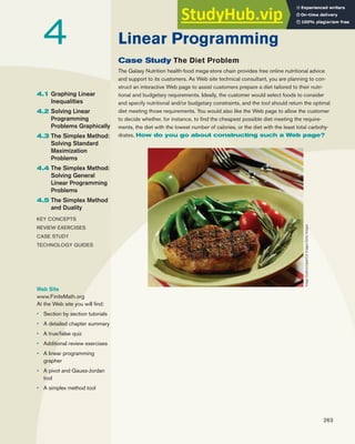
  • 1. 263 4.1 Graphing Linear Inequalities 4.2 Solving Linear Programming Problems Graphically 4.3 The Simplex Method: Solving Standard Maximization Problems 4.4 The Simplex Method: Solving General Linear Programming Problems 4.5 The Simplex Method and Duality KEY CONCEPTS REVIEW EXERCISES CASE STUDY TECHNOLOGY GUIDES Linear Programming 4 Web Site www.FiniteMath.org At the Web site you will find: • Section by section tutorials • A detailed chapter summary • A true/false quiz • Additional review exercises • A linear programming grapher • A pivot and Gauss-Jordan tool • A simplex method tool Case Study The Diet Problem The Galaxy Nutrition health-food mega-store chain provides free online nutritional advice and support to its customers. As Web site technical consultant, you are planning to con- struct an interactive Web page to assist customers prepare a diet tailored to their nutri- tional and budgetary requirements. Ideally, the customer would select foods to consider and specify nutritional and/or budgetary constraints, and the tool should return the optimal diet meeting those requirements. You would also like the Web page to allow the customer to decide whether, for instance, to find the cheapest possible diet meeting the require- ments, the diet with the lowest number of calories, or the diet with the least total carbohy- drates. How do you go about constructing such a Web page? Image Studios/UpperCut Images/Getty Images
  • 2. Introduction In this chapter we begin to look at one of the most important types of problems for busi- ness and the sciences: finding the largest or smallest possible value of some quantity (such as profit or cost) under certain constraints (such as limited resources). We call such problems optimization problems because we are trying to find the best, or optimum, value. The optimization problems we look at in this chapter involve linear functions only and are known as linear programming (LP) problems. One of the main purposes of cal- culus, which you may study later, is to solve nonlinear optimization problems. Linear programming problems involving only two unknowns can usually be solved by a graphical method that we discuss in Sections 4.1 and 4.2. When there are three or more unknowns, we must use an algebraic method, as we had to do for systems of linear equations. The method we use is called the simplex method. Invented in 1947 by George B. Dantzig✱ (1914–2005), the simplex method is still the most commonly used technique to solve LP problems in real applications, from finance to the computation of trajectories for guided missiles. The simplex method can be used for hand calculations when the numbers are fairly small and the unknowns are few. Practical problems often involve large numbers and many unknowns, however. Problems such as routing telephone calls or airplane flights, or allocating resources in a manufacturing process can involve tens of thousands of un- knowns. Solving such problems by hand is obviously impractical, and so computers are regularly used. Although computer programs most often use the simplex method, math- ematicians are always seeking faster methods. The first radically different method of solving LP problems was the ellipsoid algorithm published in 1979 by the Soviet math- ematician Leonid G. Khachiyan2 (1952–2005). In 1984, Narendra Karmarkar (1957–), a researcher at Bell Labs, created a more efficient method now known as Karmarkar’s algorithm. Although these methods (and others since developed) can be shown to be faster than the simplex method in the worst cases, it seems to be true that the simplex method is still the fastest in the applications that arise in practice. Calculators and spreadsheets are very useful aids in the simplex method. In prac- tice, software packages do most of the work, so you can think of what we teach you here as a peek inside a “black box.” What the software cannot do for you is convert a real sit- uation into a mathematical problem, so the most important lessons to get out of this chapter are (1) how to recognize and set up a linear programming problem, and (2) how to interpret the results. 264 Chapter 4 Linear Programming Graphing Linear Inequalities By the end of the next section, we will be solving linear programming (LP) problems with two unknowns. We use inequalities to describe the constraints in a problem, such as limitations on resources. Recall the basic notation for inequalities. 4.1 ✱ NOTE Dantzig is the real-life source of the story of the student who, walking in late to a math class, copies down two problems on the board, thinking they’re homework. After much hard work he hands in the solutions, only to discover that he’s just solved two famous unsolved problems. This actually happened to Dantzig in graduate school in 1939.1 1 Sources: D. J. Albers and C. Reid, “An Interview of George B. Dantzig: The Father of Linear Programming,” College Math. Journal, v. 17 (1986), pp. 293–314. Quoted and discussed in the context of the urban legends it inspired at www.snopes.com/college/homework/unsolvable.asp. 2 Dantzig and Khachiyan died approximately two weeks apart in 2005. The New York Times ran their obituaries together on May 23, 2005.
  • 3. Here are the particular kinds of inequalities in which we’re interested: 4.1 Graphing Linear Inequalities 265 Linear Inequalities and Solving Inequalities An inequality in the unknown x is the statement that one expression involving x is less than or equal to (or greater than or equal to) another. Similarly, we can have an inequality in x and y, which involves expressions that contain x and y; an inequality in x, y, and z; and so on. A linear inequality in one or more unknowns is an inequality of the form ax ≤ b (or ax ≥ b), a and b real constants ax + by ≤ c (or ax + by ≥ c), a, b, and c real constants ax + by + cz ≤ d, a, b, c, and d real constants ax + by + cz + dw ≤ e, a, b, c, d, and e real constants and so on. Nonstrict Inequalities a ≤ b means that a is less than or equal to b. a ≥ b means that a is greater than or equal to b. Quick Examples 3 ≤ 99, −2 ≤ −2, 0 ≤ 3 3 ≥ 3, 1.78 ≥ 1.76, 1 3 ≥ 1 4 Rules for Manipulating Inequalities 1. The same quantity can be added to or x ≤ y implies x − 4 ≤ y − 4 subtracted from both sides of an inequality: If x ≤ y, then x + a ≤ y + a for any real number a. 2. Both sides of an inequality can be multiplied x ≤ y implies 3x ≤ 3y or divided by a positive constant: If x ≤ y and a is positive, then ax ≤ ay. 3. Both sides of an inequality can be multiplied x ≤ y implies −3x ≥ −3y or divided by a negative constant if the inequality is reversed: If x ≤ y and a is negative, then ax ≥ ay. 4. The left and right sides of an inequality can 3x ≥ 5y implies 5y ≤ 3x be switched if the inequality is reversed: If x ≤ y, then y ≥ x; if y ≥ x, then x ≤ y. There are also the inequalities < and >, called strict inequalities because they do not permit equality. We do not use them in this chapter. Following are some of the basic rules for manipulating inequalities. Although we illustrate all of them with the inequality ≤, they apply equally well to inequalities with ≥ and to the strict inequalities < and >. Quick Examples
  • 4. Solving Linear Inequalities in Two Variables Our first goal is to solve linear inequalities in two variables—that is, inequalities of the form ax + by ≤ c. As an example, let’s solve 2x + 3y ≤ 6. We already know how to solve the equation 2x + 3y = 6. As we saw in Chapter 1, the solution of this equation may be pictured as the set of all points (x, y) on the straight-line graph of the equation. This straight line has x-intercept 3 (obtained by putting y = 0 in the equation) and y-intercept 2 (obtained by putting x = 0 in the equation) and is shown in Figure 1. Notice that, if (x, y) is any point on the line, then x and y not only satisfy the equa- tion 2x + 3y = 6, but they also satisfy the inequality 2x + 3y ≤ 6, because being equal to 6 qualifies as being less than or equal to 6. Do the points on the line give all possible solutions to the inequality? No. For example, try the origin, (0, 0). Because 2(0) + 3(0) = 0 ≤ 6, the point (0, 0) is a solution that does not lie on the line. In fact, here is a possibly surprising fact: The so- lution to any linear inequality in two unknowns is represented by an entire half plane: the set of all points on one side of the line (including the line itself). Thus, because (0, 0) is a solution of 2x + 3y ≤ 6 and is not on the line, every point on the same side of the line as (0, 0) is a solution as well (the colored region below the line in Figure 2 shows which half plane constitutes the solution set). To see why the solution set of 2x + 3y ≤ 6 is the entire half plane shown, start with any point P on the line 2x + 3y = 6. We already know that P is a solution of 2x + 3y ≤ 6. If we choose any point Q directly below P, the x-coordinate of Q will be the same as that of P, and the y-coordinate will be smaller. So the value of 2x + 3y at Q will be smaller than the value at P, which is 6. Thus, 2x + 3y < 6 at Q, and so Q is an- other solution of the inequality. (See Figure 3.) In other words, every point beneath the line is a solution of 2x + 3y ≤ 6. On the other hand, any point above the line is directly above a point on the line, and so 2x + 3y > 6 for such a point. Thus, no point above the line is a solution of 2x + 3y ≤ 6. 266 Chapter 4 Linear Programming A solution of an inequality in the unknown x is a value for x that makes the inequal- ity true. For example, 2x + 8 ≥ 89 has a solution x = 50 because 2(50) + 8 ≥ 89. Of course, it has many other solutions as well. Similarly, a solution of an inequality in x and y is a pair of values (x, y) making the inequality true. For example, (5, 1) is a solution of 3x − 2y ≥ 8 because 3(5) − 2(1) ≥ 8. To solve an inequality is to find the set of all solutions. Quick Examples 2x + 8 ≥ 89+ Linear inequality in x 2x3 ≤ x3 + y Nonlinear inequality in x and y 3x − 2y ≥ 8 Linear inequality in x and y x2 + y2 ≤ 19z Nonlinear inequality in x, y, and z 3x − 2y + 4z ≤ 0 Linear inequality in x, y, and z Figure 1 x y 2x ⫹ 3y ⫽ 6 Figure 2 x y 2x ⫹ 3y ⫽ 6 (0, 0) Solution Set Figure 3 x y 2x ⫹ 3y ⫽ 6 2x ⫹ 3y ⬍ 6 Q P(x, y)
  • 5. The same kind of argument can be used to show that the solution set of every in- equality of the form ax + by ≤ c or ax + by ≥ c consists of the half plane above or below the line ax + by = c. The “test-point” procedure we describe below gives us an easy method for deciding whether the solution set includes the region above or below the corresponding line. Now we are going to do something that will appear backward at first (but makes it simpler to sketch sets of solutions of systems of linear inequalities). For our standard drawing of the region of solutions of 2x + 3y ≤ 6, we are going to shade only the part that we do not want and leave the solution region blank. Think of covering over or “blocking out” the unwanted points, leaving those that we do want in full view (but re- member that the points on the boundary line are also points that we want). The result is Figure 4. The reason we do this should become clear in Example 2. 4.1 Graphing Linear Inequalities 267 Figure 4 x y (0, 0) Solution Set 2x ⫹ 3y ⫽ 6 Sketching the Region Represented by a Linear Inequality in Two Variables 1. Sketch the straight line obtained by replacing the given inequality with an equality. 2. Choose a test point not on the line; (0, 0) is a good choice if the line does not pass through the origin. 3. If the test point satisfies the inequality, then the set of solutions is the entire region on the same side of the line as the test point. Otherwise, it is the region on the other side of the line. In either case, shade (block out) the side that does not contain the solutions, leaving the solution set unshaded. Quick Example Here are the three steps used to graph the inequality x + 2y ≥ 5. x Solution Set y x ⫹ 2y ⫽ 5 x y x ⫹ 2y ⫽ 5 Test Point (0, 0) x y x ⫹ 2y ⫽ 5 1. Sketch the line x + 2y = 5. 2. Test the point (0, 0) 0 + 2(0) 5 Inequality is not satisfied. 3. Because the inequality is not satisfied, shade the region containing the test point. EXAMPLE 1 Graphing Single Inequalities Sketch the regions determined by each of the following inequalities: a. 3x − 2y ≤ 6 b. 6x ≤ 12 + 4y c. x ≤ −1 d. y ≥ 0 e. x ≥ 3y
  • 6. c. The region x ≤ −1 has as boundary the vertical line x = −1. The test point (0, 0) is not in the solution set, as shown in Figure 6. d. The region y ≥ 0 has as boundary the horizontal line y = 0 (that is, the x-axis). We cannot use (0, 0) for the test point because it lies on the boundary line. Instead, we choose a convenient point not on the line y = 0—say, (0, 1). Because 1 ≥ 0, this point is in the solution set, giving us the region shown in Figure 7. e. The line x ≥ 3y has as boundary the line x = 3y or, solving for y, y = 1 3 x. This line passes through the origin with slope 1/3, so again we cannot choose the ori- gin as a test point. Instead, we choose (0, 1). Substituting these coordinates in x ≥ 3y gives 0 ≥ 3(1), which is false, so (0, 1) is not in the solution set, as shown in Figure 8. 268 Chapter 4 Linear Programming using Technology Technology can be used to graph inequalities. Here is an outline (see the Technology Guides at the end of the chapter for additional details on using a TI-83/84 Plus or Excel): TI-83/84 Plus Solve the inequality for y and enter the resulting function of x; for example, Y1=-(2/3)*X+2. Position the cursor on the icon to the left of Y1 and press until you see the kind of shading desired (above or below the line). [More details on page 343.] Excel Solve the inequality for y and create a scattergraph using two points on the line. Then use the drawing palette to create a polygon to provide the shading. [More details on page 345.] Web Site www.FiniteMath.org Online Utilities Linear Programming Grapher Type “graph” and enter one or more inequalities (each one on a new line) as shown: Adjust the graph window set- tings, and click “Graph.” ENTER Solution a. The boundary line 3x − 2y = 6 has x-intercept 2 and y-intercept −3 (Figure 5). We use (0, 0) as a test point (because it is not on the line). Because 3(0) − 2(0) ≤ 6, the inequality is satisfied by the test point (0, 0), and so it lies inside the solution set. The solution set is shown in Figure 5. b. The given inequality, 6x ≤ 12 + 4y, can be rewritten in the form ax + by ≤ c by subtracting 4y from both sides: 6x − 4y ≤ 12. Dividing both sides by 2 gives the inequality 3x − 2y ≤ 6, which we considered in part (a). Now, applying the rules for manipulating inequalities does not affect the set of solutions. Thus, the inequality 6x ≤ 12 + 4y has the same set of solutions as 3x − 2y ≤ 6. (See Figure 5.) Figure 5 x y 3x ⫺ 2y ⫽ 6 (0, 0) Solution Set Figure 6 x y x ⫽ ⫺1 Solution Set (0, 0) Figure 7 x y Solution Set (0, 1) 0 y ⫽ 0 Figure 8 x y Solution Set (0, 1) 1 3 y ⫽ x
  • 7. 4.1 Graphing Linear Inequalities 269 EXAMPLE 2 Graphing Simultaneous Inequalities Sketch the region of points that satisfy both inequalities: 2x − 5y ≤ 10 x + 2y ≤ 8. Solution Each inequality has a solution set that is a half plane. If a point is to satisfy both inequalities, it must lie in both sets of solutions. Put another way, if we cover the points that are not solutions to 2x − 5y ≤ 10 and then also cover the points that are not solutions to x + 2y ≤ 8, the points that remain uncovered must be the points we want, those that are solutions to both inequalities. The result is shown in Figure 9, where the unshaded region is the set of solutions.✱ As a check, we can look at points in various regions in Figure 9. For example, our graph shows that (0, 0) should satisfy both inequalities, and it does; 2(0) − 5(0) = 0 ≤ 10 0 + 2(0) = 0 ≤ 8. On the other hand, (0, 5) should fail to satisfy one of the inequalities. 2(0) − 5(5) = −25 ≤ 10 0 + 2(5) = 10 8 One more: (5, −1) should fail one of the inequalities: 2(5) − 5(−1) = 15 10 5 + 2(−1) = 3 ≤ 8. Figure 9 Solution Set x y 2x ⫺ 5y ⫽ 10 x ⫹ 2y ⫽ 8 Figure 10 x y 3x⫺ 2y⫽ 6 x ⫹ y ⫽ ⫺5 y ⫽ 4 A B C 4 2 ⫺5 ⫺5 ✔ ✔ ✔ ✗ ✗ ✔ ✱ TECHNOLOGY NOTE Although these graphs are quite easy to do by hand, the more lines we have to graph the more difficult it becomes to get everything in the right place, and this is where graphing technology can become important. This is especially true when, for instance, three or more lines intersect in points that are very close together and hard to distinguish in hand-drawn graphs. EXAMPLE 3 Corner Points Sketch the region of solutions of the following system of inequalities and list the coor- dinates of all the corner points. 3x − 2y ≤ 6 x + y ≥ −5 y ≤ 4 Solution Shading the regions that we do not want leaves us with the triangle shown in Figure 10. We label the corner points A, B, and C as shown. Each of these corner points lies at the intersection of two of the bounding lines. So, to find the coordinates of each corner point, we need to solve the system of equations given by the two lines. To do this systematically, we make the following table: Point Lines through Point Coordinates A y = 4 (−9, 4) x + y = −5 B y = 4 14 3 , 4 3x − 2y = 6 C x + y = −5 − 4 5 , − 21 5 3x − 2y = 6
  • 8. Take another look at the regions of solutions in Examples 2 and 3 (Figure 11). 270 Chapter 4 Linear Programming ✱ TECHNOLOGY NOTE Using the trace feature makes it easy to locate corner points graphically. Remember to zoom in for additional accuracy when appropriate. Of course, you can also use technology to help solve the systems of equations, as we discussed in Chapter 2. Here, we have solved each system of equations in the middle column to get the point on the right, using the techniques of Chapter 2. You should do this for practice.✱ As a partial check that we have drawn the correct region, let us choose any point in its interior—say, (0, 0). We can easily check that (0, 0) satisfies all three given inequalities. It follows that all of the points in the triangular region containing (0, 0) are also solutions. Figure 11 Solution Set x y x y Solution Set (a) Example 2 Solution Set (b) Example 3 Solution Set Notice that the solution set in Figure 11(a) extends infinitely far to the left, whereas the one in Figure 11(b) is completely enclosed by a boundary. Sets that are completely enclosed are called bounded, and sets that extend infinitely in one or more directions are unbounded. For example, all the solution sets in Example 1 are unbounded. EXAMPLE 4 Resource Allocation Socaccio Pistachio Inc. makes two types of pistachio nuts: Dazzling Red and Organic. Pistachio nuts require food color and salt, and the following table shows the amount of food color and salt required for a 1-kilogram batch of pistachios, as well as the total amount of these ingredients available each day. Use a graph to show the possible numbers of batches of each type of pistachio Socaccio can produce each day. This region (the solution set of a system of inequalities) is called the feasible region. Solution As we did in Chapter 2, we start by identifying the unknowns: Let x be the number of batches of Dazzling Red manufactured per day and let y be the number of batches of Organic manufactured each day. Now, because of our experience with systems of linear equations, we are tempted to say: For food color 2x + y = 20 and for salt, 10x + 20y = 220. However, no one is say- ing that Socaccio has to use all available ingredients; the company might choose to use fewer than the total available amounts if this proves more profitable. Thus, 2x + y can be anything up to a total of 20. In other words, 2x + y ≤ 20. Similarly, 10x + 20y ≤ 220. Dazzling Red Organic Total Available Food Color (g) 2 1 20 Salt (g) 10 20 220
  • 9. Before we go on... Every point in the feasible region in Example 4 represents a value for x and a value for y that do not violate any of the company’s restrictions. For example, the point (5, 6) lies well inside the region, so the company can produce five batches of Dazzling Red nuts and six batches of Organic without exceeding the limitations on ingredients [that is, 2(5) + 6 = 16 ≤ 20 and 10(5) + 20(6) = 170 ≤ 220]. The corner points A, B, C, and D are significant if the company wishes to realize the greatest profit, as we will see in Section 4.2. We can find the corners as in the following table: ➡ 4.1 Graphing Linear Inequalities 271 There are two more restrictions not explicitly mentioned: Neither x nor y can be nega- tive. (The company cannot produce a negative number of batches of nuts.) Therefore, we have the additional restrictions x ≥ 0 y ≥ 0. These two inequalities tell us that the feasible region (solution set) is restricted to the first quadrant, because in the other quadrants, either x or y or both x and y are negative. So instead of shading out all other quadrants, we can simply restrict our drawing to the first quadrant. The (bounded) feasible region shown in Figure 12 is a graphical representation of the limitations the company faces. Figure 12 x y 10x ⫹ 20y ⫽ 220 2x ⫹ y ⫽ 20 A D C B Feasible Region 20 11 10 22 (We have not listed the lines through the first three corners because their coordi- nates can be read easily from the graph.) Points on the line segment DB represent use of all the food color (because the segment lies on the line 2x + y = 20), and points on the line segment C D represent use of all the salt (because the segment lies on the line 10x + 20y = 220). Note that the point D is the only solution that uses all of both ingredients. 쮿 Point Lines through Point Coordinates A (0, 0) B (10, 0) C (0, 11) D 2x + y = 20 (6, 8) 10x + 20y = 220 Recognizing Whether to Use a Linear Inequality or a Linear Equation How do I know whether to model a situation by a linear inequality like 3x + 2y ≤ 10 or by a linear equation like 3x + 2y = 10? Here are some key phrases to look for: at most, up to, no more than, at least, or more, exactly. Suppose, for instance, that nuts cost 3¢, bolts cost 2¢, x is the number of nuts you can buy, and y is the number of bolts you can buy. • If you have up to 10¢ to spend, then 3x + 2y ≤ 10. • If you must spend exactly 10¢, then 3x + 2y = 10. • If you plan to spend at least 10¢, then 3x + 2y ≥ 10. The use of inequalities to model a situation is often more realistic than the use of equations; for instance, one cannot always expect to exactly fill all orders, spend the exact amount of one’s budget, or keep a plant operating at exactly 100% capacity.
  • 10. 272 Chapter 4 Linear Programming In Exercises 27–32, we suggest you use technology. Graph the regions corresponding to the inequalities, and find the coordinates of all corner points (if any) to two decimal places: 27. 2.1x − 4.3y ≥ 9.7 28. −4.3x + 4.6y ≥ 7.1 29. −0.2x + 0.7y ≥ 3.3 1.1x + 3.4y ≥ 0 30. 0.2x + 0.3y ≥ 7.2 2.5x − 6.7y ≤ 0 31. 4.1x − 4.3y ≤ 4.4 7.5x − 4.4y ≤ 5.7 4.3x + 8.5y ≤ 10 32. 2.3x − 2.4y ≤ 2.5 4.0x − 5.1y ≤ 4.4 6.1x + 6.7y ≤ 9.6 APPLICATIONS 33. Resource Allocation You manage an ice cream factory that makes two flavors: Creamy Vanilla and Continental Mocha. Into each quart of Creamy Vanilla go 2 eggs and 3 cups of cream. Into each quart of Continental Mocha go 1 egg and 3 cups of cream. You have in stock 500 eggs and 900 cups of cream. Draw the feasible region showing the number of quarts of vanilla and number of quarts of mocha that can be produced. Find the corner points of the region. HINT [See Example 4.] 34. Resource Allocation Podunk Institute of Technology’s Math Department offers two courses: Finite Math and Applied Cal- culus. Each section of Finite Math has 60 students, and each section of Applied Calculus has 50. The department is al- lowed to offer a total of up to 110 sections. Furthermore, no more than 6,000 students want to take a math course. (No stu- dent will take more than one math course.) Draw the feasible region that shows the number of sections of each class that can be offered. Find the corner points of the region. HINT [See Example 4.] 35. Nutrition Ruff Inc. makes dog food out of chicken and grain. Chicken has 10 grams of protein and 5 grams of fat per ounce, and grain has 2 grams of protein and 2 grams of fat per ounce. A bag of dog food must contain at least 200 grams of protein and at least 150 grams of fat. Draw the feasible region that shows the number of ounces of chicken and number of ounces of grain Ruff can mix into each bag of dog food. Find the cor- ner points of the region. 36. Purchasing Enormous State University’s Business School is buying computers. The school has two models to choose from: the Pomegranate and the iZac. Each Pomegranate comes with 400 MB of memory and 80 GB of disk space, and each iZac has 300 MB of memory and 100 GB of disk space. For reasons related to its accreditation, the school would like to be able to say that it has a total of at least 48,000 MB of memory and at least 12,800 GB of disk space. Draw the fea- sible region that shows the number of each kind of computer it can buy. Find the corner points of the region. 왔 more advanced ◆ challenging indicates exercises that should be solved using technology In Exercises 1–26, sketch the region that corresponds to the given inequalities, say whether the region is bounded or unbounded, and find the coordinates of all corner points (if any). HINT [See Example 1.] 1. 2x + y ≤ 10 2. 4x − y ≤ 12 3. −x − 2y ≤ 8 4. −x + 2y ≥ 4 5. 3x + 2y ≥ 5 6. 2x − 3y ≤ 7 7. x ≤ 3y 8. y ≥ 3x 9. 3x 4 − y 4 ≤ 1 10. x 3 + 2y 3 ≥ 2 11. x ≥ −5 12. y ≤ −4 13. 4x − y ≤ 8 x + 2y ≤ 2 14. 2x + y ≤ 4 x − 2y ≥ 2 HINT [See Examples 2 and 3.] HINT [See Examples 2 and 3.] 15. 3x + 2y ≥ 6 3x − 2y ≤ 6 x ≥ 0 16. 3x + 2y ≤ 6 3x − 2y ≥ 6 −y ≥ 2 17. x + y ≥ 5 x ≤ 10 y ≤ 8 x ≥ 0, y ≥ 0 18. 2x + 4y ≥ 12 x ≤ 5 y ≤ 3 x ≥ 0, y ≥ 0 19. 20x + 10y ≤ 100 10x + 20y ≤ 100 10x + 10y ≤ 60 x ≥ 0, y ≥ 0 20. 30x + 20y ≤ 600 10x + 40y ≤ 400 20x + 30y ≤ 450 x ≥ 0, y ≥ 0 21. 20x + 10y ≥ 100 10x + 20y ≥ 100 10x + 10y ≥ 80 x ≥ 0, y ≥ 0 22. 30x + 20y ≥ 600 10x + 40y ≥ 400 20x + 30y ≥ 600 x ≥ 0, y ≥ 0 23. −3x + 2y ≤ 5 3x − 2y ≤ 6 x ≤ 2y x ≥ 0, y ≥ 0 24. −3x + 2y ≤ 5 3x − 2y ≥ 6 y ≤ x/2 x ≥ 0, y ≥ 0 25. 2x − y ≥ 0 x − 3y ≤ 0 x ≥ 0, y ≥ 0 26. −x + y ≥ 0 4x − 3y ≥ 0 x ≥ 0, y ≥ 0 4.1 EXERCISES
  • 11. 37. Nutrition Each serving of Gerber Mixed Cereal for Baby contains 60 calories and 11 grams of carbohydrates, and each serving of Gerber Mango Tropical Fruit Dessert contains 80 calories and 21 grams of carbohydrates.3 You want to pro- vide your child with at least 140 calories and at least 32 grams of carbohydrates. Draw the feasible region that shows the num- ber of servings of cereal and number of servings of dessert that you can give your child. Find the corner points of the region. 38. Nutrition Each serving of Gerber Mixed Cereal for Baby contains 60 calories, 11 grams of carbohydrates, and no vita- min C. Each serving of Gerber Apple Banana Juice contains 60 calories, 15 grams of carbohydrates, and 120 percent of the U.S. Recommended Daily Allowance (RDA) of vitamin C for infants.4 You want to provide your child with at least 120 calories, at least 26 grams of carbohydrates, and at least 50 percent of the U.S. RDA of vitamin C for infants. Draw the feasible region that shows the number of servings of cereal and number of servings of juice that you can give your child. Find the corner points of the region. 39. Municipal Bond Funds The Pimco New York Municipal Bond Fund (PNF) and the Fidelity Spartan Mass Fund (FDMMX) are tax-exempt municipal bond funds. In 2003, the Pimco fund yielded 6% while the Fidelity fund yielded 5%.5 You would like to invest a total of up to $80,000 and earn at least $4,200 in interest in the coming year (based on the given yields). Draw the feasible region that shows how much money you can invest in each fund. Find the corner points of the region. 40. Municipal Bond Funds In 2003, the Fidelity Spartan Mass Fund (FDMMX) yielded 5%, and the Fidelity Spartan Florida Fund (FFLIX) yielded 7%.6 You would like to invest a total of up to $60,000 and earn at least $3,500 in interest. Draw the feasible region that shows how much money you can invest in each fund (based on the given yields). Find the corner points of the region. 41. 왔 Investments Your portfolio manager has suggested two high-yielding stocks: Consolidated Edison (ED) and General Electric (GE). ED shares cost $40 and yield 6% in dividends. GE shares cost $16 and yield 7.5% in dividends.7 You have up to $10,000 to invest, and would like to earn at least $600 in div- idends. Draw the feasible region that shows how many shares in each company you can buy. Find the corner points of the re- gion. (Round each coordinate to the nearest whole number.) 42. 왔 Investments Your friend’s portfolio manager has suggested two energy stocks: Exxon Mobil (XOM) and British Petroleum (BP). XOM shares cost $80 and yield 2% in dividends. BP 4.1 Graphing Linear Inequalities 273 shares cost $50 and yield 7% in dividends.8 Your friend has up to $40,000 to invest, and would like to earn at least $1,400 in dividends. Draw the feasible region that shows how many shares in each company she can buy. Find the corner points of the region. (Round each coordinate to the nearest whole number.) 43. 왔 Advertising You are the marketing director for a company that manufactures bodybuilding supplements and you are planning to run ads in Sports Illustrated and GQ Magazine. Based on readership data, you estimate that each one-page ad in Sports Illustrated will be read by 650,000 people in your target group, while each one-page ad in GQ will be read by 150,000.9 You would like your ads to be read by at least three million people in the target group and, to ensure the broadest possible audience, you would like to place at least three full- page ads in each magazine. Draw the feasible region that shows how many pages you can purchase in each magazine. Find the corner points of the region. (Round each coordinate to the nearest whole number.) 44. 왔 Advertising You are the marketing director for a company that manufactures bodybuilding supplements and you are planning to run ads in Sports Illustrated and Muscle and Fit- ness. Based on readership data, you estimate that each one- page ad in Sports Illustrated will be read by 650,000 people in your target group, while each one-page ad in Muscle and Fitness will be read by 250,000 people in your target group.10 You would like your ads to be read by at least four million people in the target group and, to ensure the broadest possible audience, you would like to place at least three full-page ads in each magazine during the year. Draw the feasible region showing how many pages you can purchase in each magazine. Find the corner points of the region. (Round each coordinate to the nearest whole number.) COMMUNICATION AND REASONING EXERCISES 45. Find a system of inequalities whose solution set is unbounded. 46. Find a system of inequalities whose solution set is empty. 47. How would you use linear inequalities to describe the triangle with corner points (0, 0), (2, 0), and (0, 1)? 48. Explain the advantage of shading the region of points that do not satisfy the given inequalities. Illustrate with an example. 49. Describe at least one drawback to the method of finding the corner points of a feasible region by drawing its graph, when the feasible region arises from real-life constraints. 3 Source: Nutrition information printed on the jar. 4 Ibid. 5 Yields are rounded. Sources: www.pimcofunds.com, www.fidelity.com. January 18, 2004. 6 Yields are rounded. Source: www.fidelity.com. January 18, 2004. 7 Share prices and yields are approximate (2008). Source: http://finance .google.com. 8 Ibid. 9 The readership data for Sports Illustrated is based, in part, on the results of a readership survey taken in March 2000. The readership data for GQ is fictitious. Source: Mediamark Research Inc./NewYork Times, May 29, 2000, p. C1. 10 The readership data for both magazines are based on the results of a readership survey taken in March 2000. Source: Mediamark Research Inc./NewYork Times, May 29, 2000, p. C1.
  • 12. 50. Draw several bounded regions described by linear inequali- ties. For each region you draw, find the point that gives the greatest possible value of x + y. What do you notice? In Exercises 51–54, you are mixing x grams of ingredient A and y grams of ingredient B. Choose the equation or inequality that models the given requirement. 51. There should be at least 3 more grams of ingredient A than ingredient B. (A) 3x − y ≤ 0 (B) x − 3y ≥ 0 (C) x − y ≥ 3 (D) 3x − y ≥ 0 52. The mixture should contain at least 25% of ingredient A by weight. (A) 4x − y ≤ 0 (B) x − 4y ≥ 0 (C) x − y ≥ 4 (D) 3x − y ≥ 0 53. 왔 There should be at least 3 parts (by weight) of ingredient A to 2 parts of ingredient B. (A) 3x − 2y ≥ 0 (B) 2x − 3y ≥ 0 (C) 3x + 2y ≥ 0 (D) 2x + 3y ≥ 0 54. 왔 There should be no more of ingredient A (by weight) than ingredient B. (A) x − y = 0 (B) x − y ≤ 0 (C) x − y ≥ 0 (D) x + y ≥ y 274 Chapter 4 Linear Programming 55. 왔 You are setting up a system of inequalities in the unknowns x and y. The inequalities represent constraints faced by Fly-by- Night Airlines, where x represents the number of first-class tickets it should issue for a specific flight and y represents the number of business-class tickets it should issue for that flight. You find that the feasible region is empty. How do you inter- pret this? 56. 왔 In the situation described in the preceding exercise, is it possible instead for the feasible region to be unbounded? Explain your answer. 57. 왔 Create an interesting scenario that leads to the following system of inequalities: 20x + 40y ≤ 1,000 30x + 20y ≤ 1,200 x ≥ 0, y ≥ 0. 58. 왔 Create an interesting scenario that leads to the following system of inequalities: 20x + 40y ≥ 1,000 30x + 20y ≥ 1,200 x ≥ 0, y ≥ 0. Solving Linear Programming Problems Graphically As we saw in Example 4 in Section 4.1, in some scenarios the possibilities are restricted by a system of linear inequalities. In that example, it would be natural to ask which of the various possibilities gives the company the largest profit. This is a kind of problem known as a linear programming problem (commonly referred to as an LP problem). 4.2 Linear Programming (LP) Problems A linear programming problem in two unknowns x and y is one in which we are to find the maximum or minimum value of a linear expression ax + by called the objective function, subject to a number of linear constraints of the form cx + dy ≤ e or cx + dy ≥ e. The largest or smallest value of the objective function is called the optimal value, and a pair of values of x and y that gives the optimal value constitutes an optimal solution.
  • 13. The set of points (x, y) satisfying all the constraints is the feasible region for the problem. Our methods of solving LP problems rely on the following facts: 4.2 Solving Linear Programming Problems Graphically 275 Quick Example Maximize p = x + y Objective function subject to x + 2y ≤ 12 2x + y ≤ 12 x ≥ 0, y ≥ 0. Constraints See Example 1 for a method of solving this LP problem (that is, finding an optimal solution and value). Fundamental Theorem of Linear Programming • If an LP problem has optimal solutions, then at least one of these solutions occurs at a corner point of the feasible region. • Linear programming problems with bounded, nonempty feasible regions always have optimal solutions. Let’s see how we can use this to solve an LP problem, and then we’ll discuss why it’s true. EXAMPLE 1 Solving an LP Problem Maximize p = x + y subject to x + 2y ≤ 12 2x + y ≤ 12 x ≥ 0, y ≥ 0. Solution We begin by drawing the feasible region for the problem. We do this using the techniques of Section 4.1, and we get Figure 13. Each feasible point (point in the feasible region) gives an x and a y satisfying the constraints. The question now is, which of these points gives the largest value of the ob- jective function p = x + y? The Fundamental Theorem of Linear Programming tells us that the largest value must occur at one (or more) of the corners of the feasible region. In the following table, we list the coordinates of each corner point and we compute the value of the objective function at each corner. Figure 13 x y x ⫹ 2y ⫽ 12 2x ⫹ y ⫽ 12 12 6 6 12 A D C B Feasible Region Corner Point Lines through Point Coordinates p = x + y A (0, 0) 0 B (6, 0) 6 C (0, 6) 6 D x + 2y = 12 (4, 4) 8 2x + y = 12 Now we simply pick the one that gives the largest value for p, which is D. Therefore, the optimal value of p is 8, and an optimal solution is (4, 4).
  • 14. Now we owe you an explanation of why one of the corner points should be an optimal solution. The question is, which point in the feasible region gives the largest possible value of p = x + y? Consider first an easier question: Which points result in a particular value of p? For example, which points result in p = 2? These would be the points on the line x + y = 2, which is the line labeled p = 2 in Figure 14. Now suppose we want to know which points make p = 4: These would be the points on the line x + y = 4, which is the line labeled p = 4 in Figure 14. Notice that this line is parallel to but higher than the line p = 2. (If p represented profit in an appli- cation, we would call these isoprofit lines, or constant-profit lines.) Imagine moving this line up or down in the picture. As we move the line down, we see smaller values of p, and as we move it up, we see larger values. Several more of these lines are drawn in Figure 14. Look, in particular, at the line labeled p = 10. This line does not meet the feasible region, meaning that no feasible point makes p as large as 10. Starting with the line p = 2, as we move the line up, increasing p, there will be a last line that meets the feasible region. In the figure it is clear that this is the line p = 8, and this meets the feasible region in only one point, which is the corner point D. Therefore, D gives the greatest value of p of all feasible points. If we had been asked to maximize some other objective function, such as p = x + 3y, then the optimal solution might be different. Figure 15 shows some of the isoprofit lines for this objective function. This time, the last point that is hit as p increases is C, not D. This tells us that the optimal solution is (0, 6), giving the optimal value p = 18. This discussion should convince you that the optimal value in an LP problem will always occur at one of the corner points. By the way, it is possible for the optimal value to occur at two corner points and at all points along an edge connecting them. (Do you see why?) We will see this in Example 3(b). Here is a summary of the method we have just been using. 276 Chapter 4 Linear Programming Figure 14 p ⫽ 10 x y A p ⫽ 8 p ⫽ 6 p ⫽ 4 p ⫽ 2 B D C p ⫽ x ⫹ y Figure 15 x y p ⫽ 18 p ⫽ 12 p ⫽ 6 A D C B p ⫽ x ⫹ 3y Graphical Method for Solving Linear Programming Problems in Two Unknowns (Bounded Feasible Regions) 1. Graph the feasible region and check that it is bounded. 2. Compute the coordinates of the corner points. 3. Substitute the coordinates of the corner points into the objective function to see which gives the maximum (or minimum) value of the objective function. 4. Any such corner point is an optimal solution. Note If the feasible region is unbounded, this method will work only if there are optimal solutions; otherwise, it will not work. We will show you a method for deciding this on page 280. 쮿 APPLICATIONS EXAMPLE 2 Resource Allocation Acme Babyfoods mixes two strengths of apple juice. One quart of Beginner’s juice is made from 30 fluid ounces of water and 2 fluid ounces of apple juice concentrate. One quart of Advanced juice is made from 20 fluid ounces of water and 12 fluid ounces of
  • 15. 4.2 Solving Linear Programming Problems Graphically 277 Figure 16 x y x ⫹ 6y ⫽ 1,800 A D C B Feasible Region 3x ⫹ 2y ⫽ 3,000 1,500 1,000 1,800 300 concentrate. Every day Acme has available 30,000 fluid ounces of water and 3,600 fluid ounces of concentrate. Acme makes a profit of 20¢ on each quart of Beginner’s juice and 30¢ on each quart of Advanced juice. How many quarts of each should Acme make each day to get the largest profit? How would this change if Acme made a profit of 40¢ on Beginner’s juice and 20¢ on Advanced juice? Solution Looking at the question that we are asked, we see that our unknown quanti- ties are x = number of quarts of Beginner’s juice made each day y = number of quarts of Advanced juice made each day. (In this context, x and y are often called the decision variables, because we must decide what their values should be in order to get the largest profit.) We can write down the data given in the form of a table (the numbers in the first two columns are amounts per quart of juice): Beginner’s, x Advanced, y Available Water (ounces) 30 20 30,000 Concentrate (ounces) 2 12 3,600 Profit (¢) 20 30 Because nothing in the problem says that Acme must use up all the water or concentrate, just that it can use no more than what is available, the first two rows of the table give us two inequalities: 30x + 20y ≤ 30,000 2x + 12y ≤ 3,600. Dividing the first inequality by 10 and the second by 2 gives 3x + 2y ≤ 3,000 x + 6y ≤ 1,800. We also have that x ≥ 0 and y ≥ 0 because Acme can’t make a negative amount of juice. To finish setting up the problem, we are asked to maximize the profit, which is p = 20x + 30y. Expressed in ¢ This gives us our LP problem: Maximize p = 20x + 30y subject to 3x + 2y ≤ 3,000 x + 6y ≤ 1,800 x ≥ 0, y ≥ 0. The (bounded) feasible region is shown in Figure 16. The corners and the values of the objective function are listed in the following table: Point Lines through Point Coordinates p = 20x + 30y A (0, 0) 0 B (1,000, 0) 20,000 C (0, 300) 9,000 D 3x + 2y = 3,000 (900, 150) 22,500 x + 6y = 1,800
  • 16. We can see that, in this case, Acme should make 1,000 quarts of Beginner’s juice and no Advanced juice, for a largest possible profit of 40,000¢, or $400. 278 Chapter 4 Linear Programming We are seeking to maximize the objective function p, so we look for corner points that give the maximum value for p. Because the maximum occurs at the point D, we con- clude that the (only) optimal solution occurs at D. Thus, the company should make 900 quarts of Beginner’s juice and 150 quarts of Advanced juice, for a largest possible profit of 22,500¢, or $225. If, instead, the company made a profit of 40¢ on each quart of Beginner’s juice and 20¢ on each quart of Advanced juice, then we would have p = 40x + 20y. This gives the following table: Point Lines through Point Coordinates p = 40x + 20y A (0, 0) 0 B (1,000, 0) 40,000 C (0, 300) 6,000 D 3x + 2y = 3,000 (900, 150) 39,000 x + 6y = 1,800 Before we go on... Notice that, in the first version of the problem in Example 2, the company used all the water and juice concentrate: Water: 30(900) + 20(150) = 30,000 Concentrate: 2(900) + 12(150) = 3,600. In the second version, it used all the water but not all the concentrate: Water: 30(100) + 20(0) = 30,000 Concentrate: 2(100) + 12(0) = 200 3,600. 쮿 ➡ EXAMPLE 3 Investments The Solid Trust Savings Loan Company has set aside $25 million for loans to home buyers. Its policy is to allocate at least $10 million annually for luxury condominiums. A government housing development grant it receives requires, however, that at least one-third of its total loans be allocated to low-income housing. a. Solid Trust’s return on condominiums is 12% and its return on low-income housing is 10%. How much should the company allocate for each type of housing to maximize its total return? b. Redo part (a), assuming that the return is 12% on both condominiums and low- income housing. Solution a. We first identify the unknowns: Let x be the annual amount (in millions of dollars) allocated to luxury condominiums, and let y be the annual amount allocated to low- income housing. We now look at the constraints. The first constraint is mentioned in the first sen- tence: The total the company can invest is $25 million. Thus, x + y ≤ 25. Renaud Visage/age fotostock/PhotoLibrary
  • 17. 4.2 Solving Linear Programming Problems Graphically 279 (The company is not required to invest all of the $25 million; rather, it can invest up to $25 million.) Next, the company has allocated at least $10 million to condos. Rephrasing this in terms of the unknowns, we get The amount allocated to condos is at least $10 million. The phrase “is at least” means ≥. Thus, we obtain a second constraint: x ≥ 10. The third constraint is that at least one-third of the total financing must be for low- income housing. Rephrasing this, we say: The amount allocated to low-income housing is at least one-third of the total. Because the total investment will be x + y, we get y ≥ 1 3 (x + y). We put this in the standard form of a linear inequality as follows: 3y ≥ x + y −x + 2y ≥ 0. There are no further constraints. Now, what about the return on these investments? According to the data, the an- nual return is given by p = 0.12x + 0.10y. We want to make this quantity p as large as possible. In other words, we want to Maximize p = 0.12x + 0.10y subject to x + y ≤ 25 x ≥ 10 −x + 2y ≥ 0 x ≥ 0, y ≥ 0. (Do you see why the inequalities x ≥ 0 and y ≥ 0 are slipped in here?) The feasible region is shown in Figure 17. We now make a table that gives the return on investment at each corner point: Multiply both sides by 3. Subtract x + y from both sides. From the table, we see that the values of x and y that maximize the return are x = 50/3 and y = 25/3, which give a total return of $2.833 million. In other words, the most profitable course of action is to invest $16.667 million in loans for condo- miniums and $8.333 million in loans for low-income housing, giving a maximum annual return of $2.833 million. Point Lines through Point Coordinates p = 0.12x + 0.10y A (10, 15) 2.7 B (50/3, 25/3) 2.833 C (10, 5) 1.7 x = 10 x + y = 25 x + y = 25 −x + 2y = 0 x = 10 −x + 2y = 0 Figure 17 x y ⫺x ⫹ 2y ⫽ 0 x ⫹ y ⫽ 25 B Feasible Region A C x ⫽ 10 25 10 25
  • 18. Looking at the table, we see that a curious thing has happened: We get the same max- imum annual return at both A and B. Thus, we could choose either option to maximize the annual return. In fact, any point along the line segment AB will yield an annual return of $3 million. For example, the point (12, 13) lies on the line segment AB and also yields an annual revenue of $3 million. This happens because the “isoreturn” lines are parallel to that edge. 280 Chapter 4 Linear Programming b. The LP problem is the same as for part (a) except for the objective function: Maximize p = 0.12x + 0.12y subject to x + y ≤ 25 x ≥ 10 −x + 2y ≥ 0 x ≥ 0, y ≥ 0. Here are the values of p at the three corners: Point Coordinates p = 0.12x + 0.12y A (10, 15) 3 B (50/3, 25/3) 3 C (10, 5) 1.8 Before we go on... What breakdowns of investments would lead to the lowest return for parts (a) and (b)? 쮿 The preceding examples all had bounded feasible regions. If the feasible region is unbounded, then, provided there are optimal solutions, the fundamental theorem of lin- ear programming guarantees that the above method will work. The following procedure determines whether or not optimal solutions exist and finds them when they do. ➡ Solving Linear Programming Problems in Two Unknowns (Unbounded Feasible Regions) If the feasible region of an LP problem is unbounded, proceed as follows: 1. Draw a rectangle large enough so that all the corner points are inside the rectangle (and not on its boundary): Corner points: A, B, C Corner points inside the rectangle A B C y x Unbounded Feasible Region A B C y x
  • 19. In the next two examples, we work with unbounded feasible regions. 4.2 Solving Linear Programming Problems Graphically 281 2. Shade the outside of the rectangle so as to define a new bounded feasible region, and locate the new corner points: New corner points: D, E, and F 3. Obtain the optimal solutions using this bounded feasible region. 4. If any optimal solutions occur at one of the original corner points (A, B, and C in the figure), then the LP problem has that corner point as an optimal solution. Otherwise, the LP problem has no optimal solutions. When the latter occurs, we say that the objective function is unbounded, because it can assume arbitrarily large (positive or negative) values. A D E B C F y x EXAMPLE 4 Cost You are the manager of a small store that specializes in hats, sunglasses, and other ac- cessories. You are considering a sales promotion of a new line of hats and sunglasses. You will offer the sunglasses only to those who purchase two or more hats, so you will sell at least twice as many hats as pairs of sunglasses. Moreover, your supplier tells you that, due to seasonal demand, your order of sunglasses cannot exceed 100 pairs. To en- sure that the sale items fill out the large display you have set aside, you estimate that you should order at least 210 items in all. a. Assume that you will lose $3 on every hat and $2 on every pair of sunglasses sold. Given the constraints above, how many hats and pairs of sunglasses should you order to lose the least amount of money in the sales promotion? b. Suppose instead that you lose $1 on every hat sold but make a profit of $5 on every pair of sunglasses sold. How many hats and pairs of sunglasses should you order to make the largest profit in the sales promotion? c. Now suppose that you make a profit of $1 on every hat sold but lose $5 on every pair of sunglasses sold. How many hats and pairs of sunglasses should you order to make the largest profit in the sales promotion? Solution a. The unknowns are: x = number of hats you order y = number of pairs of sunglasses you order.
  • 20. The corner point that gives the minimum value of the objective function c is B. Be- cause B is one of the corner points of the original feasible region, we conclude that our linear programming problem has an optimal solution at B. Thus, the combination that gives the smallest loss is 140 hats and 70 pairs of sunglasses. 282 Chapter 4 Linear Programming The objective is to minimize the total loss: c = 3x + 2y. Now for the constraints. The requirement that you will sell at least twice as many hats as sunglasses can be rephrased as: The number of hats is at least twice the number of pairs of sunglasses, or x ≥ 2y which, in standard form, is x − 2y ≥ 0. Next, your order of sunglasses cannot exceed 100 pairs, so y ≤ 100. Finally, you would like to sell at least 210 items in all, giving x + y ≥ 210. Thus, the LP problem is the following: Minimize c = 3x + 2y subject to x − 2y ≥ 0 y ≤ 100 x + y ≥ 210 x ≥ 0, y ≥ 0. The feasible region is shown in Figure 18. This region is unbounded, so there is no guarantee that there are any optimal solutions. Following the procedure described above, we enclose the corner points in a rectangle as shown in Figure 19. (There are many infinitely many possible rectangles we could have used. We chose one that gives convenient coordinates for the new corners.) We now list all the corners of this bounded region along with the corresponding values of the objective function c: Figure 18 x y x ⫺ 2y ⫽ 0 x ⫹ y ⫽ 210 y ⫽ 100 100 210 210 A C B Feasible Region Figure 19 100 210 B x y x ⫺ 2y ⫽ 0 x ⫹ y ⫽ 210 y ⫽ 100 A E C D 210 300 Point Lines through Point Coordinates c = 3x + 2y ($) A (210, 0) 630 B (140, 70) 560 C (200, 100) 800 D (300, 100) 1,100 E (300, 0) 900 x + y = 210 x − 2y = 0 x − 2y = 0 y = 100
  • 21. The corner point that gives the maximum value of the objective function p is C. Be- cause C is one of the corner points of the original feasible region, we conclude that our LP problem has an optimal solution at C. Thus, the combination that gives the largest profit ($300) is 200 hats and 100 pairs of sunglasses. c. The objective function is now p = x − 5y, which is the negative of the objective function used in part (b). Thus, the table of values of p is the same as in part (b), ex- cept that it has opposite signs in the p column. This time we find that the maximum value of p occurs at E. However, E is not a corner point of the original feasible region, so the LP problem has no optimal solution. Referring to Figure 18, we can make the objective p as large as we like by choosing a point far to the right in the unbounded feasible region. Thus, the objective function is unbounded; that is, it is possible to make an arbitrarily large profit. 4.2 Solving Linear Programming Problems Graphically 283 b. The LP problem is the following: Maximize p = −x + 5y subject to x − 2y ≥ 0 y ≤ 100 x + y ≥ 210 x ≥ 0, y ≥ 0. Because most of the work is already done for us in part (a), all we need to do is change the objective function in the table that lists the corner points: Point Lines through Point Coordinates p = −x + 5y ($) A (210, 0) −210 B (140, 70) 210 C (200, 100) 300 D (300, 100) 200 E (300, 0) −300 x + y = 210 x − 2y = 0 x − 2y = 0 y = 100 EXAMPLE 5 Resource Allocation You are composing a very avant-garde ballade for violins and bassoons. In your ballade, each violinist plays a total of two notes and each bassoonist only one note. To make your ballade long enough, you decide that it should contain at least 200 instrumental notes. Furthermore, after playing the requisite two notes, each violinist will sing one soprano note, while each bassoonist will sing three soprano notes.* To make the ballade suffi- ciently interesting, you have decided on a minimum of 300 soprano notes. To give your composition a sense of balance, you wish to have no more than three times as many bas- soonists as violinists. Violinists charge $200 per performance and bassoonists $400 per performance. How many of each should your ballade call for in order to minimize personnel costs? *Whether or not these musicians are capable of singing decent soprano notes will be left to chance. You reason that a few bad notes will add character to the ballade.
  • 22. From the table we see that the minimum cost occurs at B, a corner point of the original feasible region. The linear programming problem thus has an optimal solution, and the minimum cost is $44,000 per performance, employing 60 violinists and 80 bassoonists. (Quite a wasteful ballade, one might say.) 284 Chapter 4 Linear Programming Solution First, the unknowns are x = number of violinists and y = number of bas- soonists. The constraint on the number of instrumental notes implies that 2x + y ≥ 200 because the total number is to be at least 200. Similarly, the constraint on the number of soprano notes is x + 3y ≥ 300. The next one is a little tricky. As usual, we reword it in terms of the quantities x and y. The number of bassoonists should be no more than three times the number of violinists. Thus, y ≤ 3x or 3x − y ≥ 0. Finally, the total cost per performance will be c = 200x + 400y. We wish to minimize total cost. So, our linear programming problem is as follows: Minimize c = 200x + 400y subject to 2x + y ≥ 200 x + 3y ≥ 300 3x − y ≥ 0 x ≥ 0, y ≥ 0. We get the feasible region shown in Figure 20.✱ The feasible region is unbounded, and so we add a convenient rectangle as before (Figure 21). Figure 20 x y x ⫹ 3y ⫽ 300 y ⫽ 3x 2x ⫹ y ⫽ 200 A C B 200 100 100 300 Feasible Region Figure 21 x y x ⫹ 3y ⫽ 300 y ⫽ 3x 2x ⫹ y ⫽ 200 A E C D F B 200 150 100 100 300 400 Point Lines through Point Coordinates c = 200x + 400y A (40, 120) 56,000 B (60, 80) 44,000 C (300, 0) 60,000 D (50, 150) 70,000 E (400, 150) 140,000 F (400, 0) 80,000 2x + y = 200 3x − y = 0 2x + y = 200 x + 3y = 300 3x − y = 0 y = 150 ✱ NOTE In Figure 20 you can see how graphing technology would help in determining the corner points: Unless you are very confident in the accuracy of your sketch, how do you know that the line y = 3x falls to the left of the point B? If it were to fall to the right, then B would not be a corner point and the solution would be different. You could (and should) check that B satisfies the inequality 3x − y ≥ 0, so that the line falls to the left of B as shown. However, if you use a graphing calculator or computer, you can be fairly confident of the picture produced without doing further calculations.
  • 23. 4.2 Solving Linear Programming Problems Graphically 285 Recognizing a Linear Programming Problem, Setting Up Inequalities, and Dealing with Unbounded Regions How do I recognize when an application leads to an LP problem as opposed to a system of linear equations? Here are some cues that suggest an LP problem: • Key phrases suggesting inequalities rather than equalities, like at most, up to, no more than, at least, and or more. • A quantity that is being maximized or minimized (this will be the objective). Key phrases are maximum, minimum, most, least, largest, greatest, smallest, as large as possible, and as small as possible. How do I deal with tricky phrases like “there should be no more than twice as many nuts as bolts” or “at least 50% of the total should be bolts”? The easiest way to deal with phrases like this is to use the technique we discussed in Chapter 2: reword the phrases using “the number of . . . ”, as in The number of nuts (x) is no more than twice the number of bolts (y) x ≤ 2y The number of bolts is at least 50% of the total y ≥ 0.50(x + y) Do I always have to add a rectangle to deal with unbounded regions? Under some circumstances, you can tell right away whether optimal solutions exist, even when the feasible region is unbounded. Note that the following apply only when we have the constraints x ≥ 0 and y ≥ 0. 1. If you are minimizing c = ax + by with a and b non-negative, then optimal solu- tions always exist. (Examples 4(a) and 5 are of this type.) 2. If you are maximizing p = ax + by with a and b non-negative (and not both zero), then there is no optimal solution unless the feasible region is bounded. Do you see why statements (1) and (2) are true? Web Site www.FiniteMath.org For an online utility that does everything (solves linear programming problems with two unknowns and even draws the feasible region), go to the Web site and follow Online Utilities Linear Programming Grapher. 3. Minimize c = x + y 4. Minimize c = x + 2y subject to x + 2y ≥ 6 2x + y ≥ 6 x ≥ 0, y ≥ 0. subject to x + 3y ≥ 30 2x + y ≥ 30 x ≥ 0, y ≥ 0. 5. Maximize p = 3x + y 6. Maximize p = x − 2y subject to 3x − 7y ≤ 0 7x − 3y ≥ 0 x + y ≤ 10 x ≥ 0, y ≥ 0. subject to x + 2y ≤ 8 x − 6y ≤ 0 3x − 2y ≥ 0 x ≥ 0, y ≥ 0. 왔 more advanced ◆ challenging indicates exercises that should be solved using technology In Exercises 1–20, solve the LP problems. If no optimal solution exists, indicate whether the feasible region is empty or the objec- tive function is unbounded. HINT [See Example 1.] 1. Maximize p = x + y 2. Maximize p = x + 2y subject to x + 2y ≤ 9 2x + y ≤ 9 x ≥ 0, y ≥ 0. subject to x + 3y ≤ 24 2x + y ≤ 18 x ≥ 0, y ≥ 0. 4.2 EXERCISES
  • 24. 7. Maximize p = 3x + 2y subject to 0.2x + 0.1y ≤ 1 0.15x + 0.3y ≤ 1.5 10x + 10y ≤ 60 x ≥ 0, y ≥ 0. 8. Maximize p = x + 2y subject to 30x + 20y ≤ 600 0.1x + 0.4y ≤ 4 0.2x + 0.3y ≤ 4.5 x ≥ 0, y ≥ 0. 9. Minimize c = 0.2x + 0.3y subject to 0.2x + 0.1y ≥ 1 0.15x + 0.3y ≥ 1.5 10x + 10y ≥ 80 x ≥ 0, y ≥ 0. 10. Minimize c = 0.4x + 0.1y subject to 30x + 20y ≥ 600 0.1x + 0.4y ≥ 4 0.2x + 0.3y ≥ 4.5 x ≥ 0, y ≥ 0. 11. Maximize and minimize p = x + 2y subject to x + y ≥ 2 x + y ≤ 10 x − y ≤ 2 x − y ≥ −2. 12. Maximize and minimize p = 2x − y subject to x + y ≥ 2 x − y ≤ 2 x − y ≥ −2 x ≤ 10, y ≤ 10. 13. Maximize p = 2x + 3y subject to 0.1x + 0.2y ≥ 1 2x + y ≥ 10 x ≥ 0, y ≥ 0. 14. Maximize p = 3x + 2y subject to 0.1x + 0.1y ≥ 0.2 y ≤ 10 x ≥ 0, y ≥ 0. 15. Minimize c = 2x + 4y subject to 0.1x + 0.1y ≥ 1 x + 2y ≥ 14 x ≥ 0, y ≥ 0. 16. Maximize p = 2x + 3y subject to −x + y ≥ 10 x + 2y ≤ 12 x ≥ 0, y ≥ 0. 17. 왔 Minimize c = 3x − 3y subject to x 4 ≤ y y ≤ 2x 3 x + y ≥ 5 x + 2y ≤ 10 x ≥ 0, y ≥ 0. 18. 왔 Minimize c = −x + 2y subject to y ≤ 2x 3 x ≤ 3y y ≥ 4 x ≥ 6 x + y ≤ 16. 19. 왔 Maximize p = x + y subject to x + 2y ≥ 10 2x + 2y ≤ 10 2x + y ≥ 10 x ≥ 0, y ≥ 0. 20. 왔 Minimize c = 3x + y subject to 10x + 20y ≥ 100 0.3x + 0.1y ≥ 1 x ≥ 0, y ≥ 0. APPLICATIONS 21. Resource Allocation You manage an ice cream factory that makes two flavors: Creamy Vanilla and Continental Mocha. Into each quart of Creamy Vanilla go 2 eggs and 3 cups of cream. Into each quart of Continental Mocha go 1 egg and 3 cups of cream. You have in stock 500 eggs and 900 cups of cream. You make a profit of $3 on each quart of Creamy Vanilla and $2 on each quart of Continental Mocha. How many quarts of each flavor should you make in order to earn the largest profit? HINT [See Example 2.] 22. Resource Allocation Podunk Institute of Technology’s Math Department offers two courses: Finite Math and Applied Cal- culus. Each section of Finite Math has 60 students, and each section of Applied Calculus has 50. The department is allowed to offer a total of up to 110 sections. Furthermore, no more than 6,000 students want to take a math course (no stu- dent will take more than one math course). Suppose the uni- versity makes a profit of $100,000 on each section of Finite Math and $50,000 on each section of Applied Calculus (the 286 Chapter 4 Linear Programming
  • 25. profit is the difference between what the students are charged and what the professors are paid). How many sections of each course should the department offer to make the largest profit? HINT [See Example 2.] 23. Nutrition Ruff, Inc. makes dog food out of chicken and grain. Chicken has 10 grams of protein and 5 grams of fat per ounce, and grain has 2 grams of protein and 2 grams of fat per ounce. A bag of dog food must contain at least 200 grams of protein and at least 150 grams of fat. If chicken costs 10¢ per ounce and grain costs 1¢ per ounce, how many ounces of each should Ruff use in each bag of dog food in order to minimize cost? HINT [See Example 4.] 24. Purchasing Enormous State University’s Business School is buying computers. The school has two models from which to choose, the Pomegranate and the iZac. Each Pomegranate comes with 400 MB of memory and 80 GB of disk space; each iZac has 300 MB of memory and 100 GB of disk space. For reasons related to its accreditation, the school would like to be able to say that it has a total of at least 48,000 MB of memory and at least 12,800 GB of disk space. If the Pome- granate and the iZac cost $2,000 each, how many of each should the school buy to keep the cost as low as possible? HINT [See Example 4.] 25. Nutrition Each serving of Gerber Mixed Cereal for Baby con- tains 60 calories and 11 grams of carbohydrates. Each serving of Gerber Mango Tropical Fruit Dessert contains 80 calories and 21 grams of carbohydrates.11 If the cereal costs 30¢ per serving and the dessert costs 50¢ per serving, and you want to provide your child with at least 140 calories and at least 32 grams of carbohydrates, how can you do so at the least cost? (Fractions of servings are permitted.) 26. Nutrition Each serving of Gerber Mixed Cereal for Baby con- tains 60 calories, 10 grams of carbohydrates, and no vitamin C. Each serving of Gerber Apple Banana Juice contains 60 calo- ries, 15 grams of carbohydrates, and 120 percent of the U.S. Recommended Daily Allowance (RDA) of vitamin C for infants. The cereal costs 10¢ per serving and the juice costs 30¢ per serving. If you want to provide your child with at least 120 calories, at least 25 grams of carbohydrates, and at least 60 percent of the U.S. RDA of vitamin C for infants, how can you do so at the least cost? (Fractions of servings are permitted.) 27. Energy EfficiencyYou are thinking of making your home more energy efficient by replacing some of the light bulbs with com- pact fluorescent bulbs, and insulating part or all of your exterior walls. Each compact fluorescent light bulb costs $4 and saves you an average of $2 per year in energy costs, and each square foot of wall insulation costs $1 and saves you an average of $0.20 per year in energy costs.12 Your home has 60 light fittings and 1,100 sq. ft. of uninsulated exterior wall. You can spend no more than $1,200 and would like to save as much per year in en- ergy costs as possible. How many compact fluorescent light bulbs and how many square feet of insulation should you purchase? How much will you save in energy costs per year? 28. Energy Efficiency (Compare with the preceding exercise.) You are thinking of making your mansion more energy effi- cient by replacing some of the light bulbs with compact fluo- rescent bulbs, and insulating part or all of your exterior walls. Each compact fluorescent light bulb costs $4 and saves you an average of $2 per year in energy costs, and each square foot of wall insulation costs $1 and saves you an average of $0.20 per year in energy costs.13 Your mansion has 200 light fittings and 3,000 sq. ft. of uninsulated exterior wall. To impress your friends, you would like to spend as much as possible, but save no more than $800 per year in energy costs (you are proud of your large utility bills). How many compact fluorescent light bulbs and how many square feet of insulation should you pur- chase? How much will you save in energy costs per year? Creatine Supplements Exercises 29 and 30 are based on the following data on three bodybuilding supplements. (Figures shown correspond to a single serving.)14 4.2 Solving Linear Programming Problems Graphically 287 11 Source: Nutrition information printed on the containers. 12 Source: American Council for an Energy-Efficient Economy/NewYork Times, December 1, 2003, p. C6. 13 Ibid. 14 Source: Nutritional information supplied by the manufacturers (www.netrition.com). Cost per serving is approximate. Creatine Carbohydrates Taurine Alpha Lipoic Cost (g) (g) (g) Acid (mg) ($) Cell-Tech® 10 75 2 200 2.20 (MuscleTech) RiboForce HP® 5 15 1 0 1.60 (EAS) Creatine Transport® 5 35 1 100 0.60 (Kaizen) 29. You are thinking of combining Cell-Tech and RiboForce HP to obtain a 10-day supply that provides at least 80 grams of creatine and at least 10 grams of taurine, but no more than 750 grams of carbohydrates and no more than 1,000 mil- ligrams of alpha lipoic acid. How many servings of each sup- plement should you combine to meet your specifications at the least cost? 30. You are thinking of combining Cell-Tech and Creatine Trans- port to obtain a 10-day supply that provides at least 80 grams of creatine and at least 10 grams of taurine, but no more than 600 grams of carbohydrates and no more than 2,000 mil- ligrams of alpha lipoic acid. How many servings of each sup- plement should you combine to meet your specifications at the least cost? 31. Resource Allocation Your salami manufacturing plant can order up to 1,000 pounds of pork and 2,400 pounds of beef per day for use in manufacturing its two specialties: “Count Dracula Salami” and “Frankenstein Sausage.” Production of
  • 26. the Count Dracula variety requires 1 pound of pork and 3 pounds of beef for each salami, while the Frankenstein vari- ety requires 2 pounds of pork and 2 pounds of beef for every sausage. In view of your heavy investment in advertising Count Dracula Salami, you have decided that at least one- third of the total production should be Count Dracula. On the other hand, due to the health-conscious consumer climate, your Frankenstein Sausage (sold as having less beef) is earning your company a profit of $3 per sausage, while sales of the Count Dracula variety are down and it is earning your com- pany only $1 per salami. Given these restrictions, how many of each kind of sausage should you produce to maximize profits, and what is the maximum possible profit? HINT [See Example 3.] 32. Project Design The Megabuck Hospital Corp. is to build a state-subsidized nursing home catering to homeless patients as well as high-income patients. State regulations require that every subsidized nursing home must house a minimum of 1,000 homeless patients and no more than 750 high-income patients in order to qualify for state subsidies. The overall capacity of the hospital is to be 2,100 patients. The board of directors, under pressure from a neighborhood group, insists that the number of homeless patients should not exceed twice the number of high-income patients. Due to the state subsidy, the hospital will make an average profit of $10,000 per month for every homeless patient it houses, whereas the profit per high-income patient is estimated at $8,000 per month. How many of each type of patient should it house in order to maxi- mize profit? HINT [See Example 3.] 33. Television Advertising In February 2008, each episode of “American Idol” was typically seen by 28.5 million viewers, while each episode of “Back toYou” was seen by 12.3 million viewers.15 Your marketing services firm has been hired to promote Bald No More’s hair replacement process by buying at least 30 commercial spots during episodes of “American Idol” and “Back to You.” The cable company running “Amer- ican Idol” has quoted a price of $3,000 per spot, while the cable company showing “Back to You” has quoted a price of $1,000 per spot. Bald No More’s advertising budget for TV commercials is $120,000, and it would like no more than 50% of the total number of spots to appear on “Back to You.” How many spots should you purchase on each show to reach the most viewers? 34. Television Advertising In February 2002, each episode of “Boston Public” was typically seen in 7.0 million homes, while each episode of “NYPD Blue” was seen in 7.8 million homes.16 Your marketing services firm has been hired to pro- mote Gauss Jordan Sneakers by buying at least 30 commer- cial spots during episodes of “Boston Public” and “NYPD Blue.” The cable company running “Boston Public” has quoted a price of $2,000 per spot, while the cable company showing “NYPD Blue” has quoted a price of $3,000 per spot. Gauss Jordan Sneakers’ advertising budget for TV commer- cials is $70,000, and it would like at least 75% of the total number of spots to appear on “Boston Public.” How many spots should you purchase on each show to reach the most homes? Investing Exercises 35 and 36 are based on the following data on four stocks.17 288 Chapter 4 Linear Programming 15 Ratings are for February 26, 2008. Source: Nielsen Media Research (www.tvbythenumbers.com). 16 Ratings are for February 18–24, 2002. Source: Nielsen Media Research (www.ptd.net) February 28, 2002. 17 Approximate trading price in fourth quarter of 2008 based on 50-day averages. Earnings per share are rounded. Source: http://finance .google.com. 18 Share prices and yields are approximate (2008). Source: http://finance .google.com. 19 Ibid. Earnings Price DividendYield per Share ATRI (Atrion) $90 1% $7.50 BBY (Best Buy) 20 2 3.20 IMCL 70 0 −0.70 (ImClone Systems) TR (Tootsie Roll) 25 1 0.80 35. 왔 You are planning to invest up to $10,000 in ATRI and BBY shares.You want your investment to yield at least $120 in div- idends and you want to maximize the total earnings. How many shares of each company should you purchase? 36. 왔 You are planning to invest up to $43,000 in IMCL and TR shares. For tax reasons, you want your investment to yield no more than $10 in dividends. You want to maximize the total earnings. How many shares of each company should you purchase? 37. 왔 Investments Your portfolio manager has suggested two high-yielding stocks: Consolidated Edison (ED) and General Electric (GE). ED shares cost $40, yield 6% in dividends, and have a risk index of 2.0 per share. GE shares cost $16, yield 7.5% in dividends, and have a risk index of 3.0 per share.18 You have up to $10,000 to invest, and would like to earn at least $600 in dividends. How many shares (to the nearest tenth of a unit) of each stock should you purchase to meet your requirements and minimize the total risk index for your portfolio? What is the minimum total risk index? 38. 왔 Investments Your friend’s portfolio manager has suggested two energy stocks: Exxon Mobil (XOM) and British Petroleum (BP). XOM shares cost $80, yield 2% in dividends, and have a risk index of 2.5. BP shares cost $50, yield 7% in dividends, and have a risk index of 4.5.19 Your friend has up to $40,000
  • 27. to invest, and would like to earn at least $1,400 in dividends. How many shares (to the nearest tenth of a unit) of each stock should she purchase to meet your requirements and minimize the total risk index for your portfolio? What is the minimum total risk index? 39. 왔 Planning My friends: I, the mighty Brutus, have decided to prepare for retirement by instructing young warriors in the arts of battle and diplomacy. For each hour spent in battle instruction, I have decided to charge 50 ducats. For each hour in diplomacy instruction I shall charge 40 ducats. Due to my advancing years, I can spend no more than 50 hours per week instructing the youths, although the great Jove knows that they are sorely in need of instruction! Due to my fondness for physical pursuits, I have decided to spend no more than one- third of the total time in diplomatic instruction. However, the present border crisis with the Gauls is a sore indication of our poor abilities as diplomats. As a result, I have decided to spend at least 10 hours per week instructing in diplomacy. Finally, to complicate things further, there is the matter of Scarlet Brew: I have estimated that each hour of battle instruction will require 10 gallons of Scarlet Brew to quench my students’ thirst, and that each hour of diplomacy instruc- tion, being less physically demanding, requires half that amount. Because my harvest of red berries has far exceeded my expectations, I estimate that I’ll have to use at least 400 gallons per week in order to avoid storing the fine brew at great expense. Given all these restrictions, how many hours per week should I spend in each type of instruction to maxi- mize my income? 40. 왔 Planning Repeat the preceding exercise with the following changes: I would like to spend no more than half the total time in diplomatic instruction, and I must use at least 600 gallons of Scarlet Brew. 41. 왔 Resource Allocation One day, Gillian the magician sum- moned the wisest of her women. “Devoted followers,” she began, “I have a quandary: As you well know, I possess great expertise in sleep spells and shock spells, but unfortunately, these are proving to be a drain on my aural energy resources; each sleep spell costs me 500 pico-shirleys of aural energy, while each shock spell requires 750 pico-shirleys. Clearly, I would like to hold my overall expenditure of aural energy to a minimum, and still meet my commitments in protecting the Sisterhood from the ever-present threat of trolls. Specif- ically, I have estimated that each sleep spell keeps us safe for an average of two minutes, while every shock spell protects us for about three minutes. We certainly require enough pro- tection to last 24 hours of each day, and possibly more, just to be safe. At the same time, I have noticed that each of my sleep spells can immobilize three trolls at once, while one of my typical shock spells (having a narrower range) can im- mobilize only two trolls at once. We are faced, my sisters, with an onslaught of 1,200 trolls per day! Finally, as you are no doubt aware, the bylaws dictate that for a Magician of the Order to remain in good standing, the number of shock spells must be between one-quarter and one-third the num- ber of shock and sleep spells combined. What do I do, oh Wise Ones?” 42. 왔 Risk Management The Grand Vizier of the Kingdom of Um is being blackmailed by numerous individuals and is having a very difficult time keeping his blackmailers from going public. He has been keeping them at bay with two kinds of payoff: gold bars from the Royal Treasury and po- litical favors. Through bitter experience, he has learned that each payoff in gold gives him peace for an average of about 1 month, while each political favor seems to earn him about a month and a half of reprieve. To maintain his flawless rep- utation in the Court, he feels he cannot afford any revela- tions about his tainted past to come to light within the next year. Thus it is imperative that his blackmailers be kept at bay for 12 months. Furthermore, he would like to keep the number of gold payoffs at no more than one-quarter of the combined number of payoffs because the outward flow of gold bars might arouse suspicion on the part of the Royal Treasurer. The Grand Vizier feels that he can do no more than seven political favors per year without arousing undue suspicion in the Court. The gold payoffs tend to deplete his travel budget. (The treasury has been subsidizing his numer- ous trips to the Himalayas.) He estimates that each gold bar removed from the treasury will cost him four trips. On the other hand because the administering of political favors tends to cost him valuable travel time, he suspects that each political favor will cost him about two trips. Now, he would obviously like to keep his blackmailers silenced and lose as few trips as possible. What is he to do? How many trips will he lose in the next year? 43. ◆ Management20 You are the service manager for a supplier of closed-circuit television systems. Your company can pro- vide up to 160 hours per week of technical service for your customers, although the demand for technical service far ex- ceeds this amount. As a result, you have been asked to de- velop a model to allocate service technicians’ time between new customers (those still covered by service contracts) and old customers (whose service contracts have expired). To en- sure that new customers are satisfied with your company’s service, the sales department has instituted a policy that at least 100 hours per week be allocated to servicing new cus- tomers. At the same time, your superiors have informed you that the company expects your department to generate at least $1,200 per week in revenues. Technical service time for new customers generates an average of $10 per hour (because much of the service is still under warranty) and for old cus- tomers generates $30 per hour. How many hours per week should you allocate to each type of customer to generate the most revenue? 4.2 Solving Linear Programming Problems Graphically 289 20 Loosely based on a similiar problem in An Introduction to Management Science (6th Ed.) by D. R. Anderson, D. J. Sweeny and T. A. Williams (West, 1991).
  • 28. 44. ◆ Scheduling21 The Scottsville Textile Mill produces several different fabrics on eight dobby looms which operate 24 hours per day and are scheduled for 30 days in the coming month. The Scottsville Textile Mill will produce only Fabric 1 and Fabric 2 during the coming month. Each dobby loom can turn out 4.63 yards of either fabric per hour. Assume that there is a monthly demand of 16,000 yards of Fabric 1 and 12,000 yards of Fabric 2. Profits are calculated as 33¢ per yard for each fab- ric produced on the dobby looms. a. Will it be possible to satisfy total demand? b. In the event that total demand is not satisfied, the Scottsville Textile Mill will need to purchase the fabrics from another mill to make up the shortfall. Its profits on resold fabrics ordered from another mill amount to 20¢ per yard for Fabric 1 and 16¢ per yard for Fabric 2. How many yards of each fabric should it produce to maximize profits? COMMUNICATION AND REASONING EXERCISES 45. If a linear programming problem has a bounded, nonempty feasible region, then optimal solutions (A) must exist (B) may or may not exist (C) cannot exist 46. If a linear programming problem has an unbounded, non- empty feasible region, then optimal solutions (A) must exist (B) may or may not exist (C) cannot exist 47. What can you say if the optimal value occurs at two adjacent corner points? 48. Describe at least one drawback to using the graphical method to solve a linear programming problem arising from a real-life situation. 49. Create a linear programming problem in two variables that has no optimal solution. 50. Create a linear programming problem in two variables that has more than one optimal solution. 51. Create an interesting scenario leading to the following linear programming problem: Maximize p = 10x + 10y subject to 20x + 40y ≤ 1,000 30x + 20y ≤ 1,200 x ≥ 0, y ≥ 0. 52. Create an interesting scenario leading to the following linear programming problem: Minimize c = 10x + 10y subject to 20x + 40y ≥ 1,000 30x + 20y ≥ 1,200 x ≥ 0, y ≥ 0. 53. 왔 Use an example to show why there may be no optimal so- lution to a linear programming problem if the feasible region is unbounded. 54. 왔 Use an example to illustrate why, in the event that an opti- mal solution does occur despite an unbounded feasible re- gion, that solution corresponds to a corner point of the feasi- ble region. 55. 왔 You are setting up an LP problem for Fly-by-Night Airlines with the unknowns x and y, where x represents the number of first-class tickets it should issue for a specific flight and y rep- resents the number of business-class tickets it should issue for that flight, and the problem is to maximize profit.You find that there are two different corner points that maximize the profit. How do you interpret this? 56. 왔 In the situation described in the preceding exercise, you find that there are no optimal solutions. How do you interpret this? 57. ◆ Consider the following example of a nonlinear program- ming problem: Maximize p = xy subject to x ≥ 0, y ≥ 0, x + y ≤ 2. Show that p is zero on every corner point, but is greater than zero at many noncorner points. 58. ◆ Solve the nonlinear programming problem in Exercise 57. 290 Chapter 4 Linear Programming The Simplex Method: Solving Standard Maximization Problems The method discussed in Section 4.2 works quite well for LP problems in two unknowns, but what about three or more unknowns? Because we need an axis for each unknown, wewouldneedtodrawgraphsinthreedimensions(wherewehave x-,y-andz-coordinates) to deal with problems in three unknowns, and we would have to draw in hyperspace to answer questions involving four or more unknowns. Given the state of technology as this book is being written, we can’t easily do this. So we need another method for solving 4.3 21 Adapted from The Calhoun Textile Mill Case by J. D. Camm, P. M. Dearing, and S. K. Tadisina as presented for case study in An Introduction to Management Science (6th Ed.) by D. R. Anderson, D. J. Sweeney, and T. A. Williams (West, 1991). Our exercise uses a subset of the data given in the cited study.
  • 29. LP problems that will work for any number of unknowns. One such method, called the simplex method, has been the method of choice since it was invented by George Dantzig in 1947. To illustrate it best, we first use it to solve only so-called standard maximization problems. 4.3 The Simplex Method: Solving Standard Maximization Problems 291 General Linear Programming (LP) Problem A linear program problem in n unknowns x1, x2, . . . , xn is one in which we are to find the maximum or minimum value of a linear objective function a1x1 + a2x2 + · · · + an xn, where a1, a2, . . . , an are numbers, subject to a number of linear constraints of the form b1x1 + b2x2 + · · · + bn xn ≤ c or b1x1 + b2x2 + · · · + bn xn ≥ c, where b1, b2, . . . , bn, c are numbers. Standard Maximization Problem A standard maximization problem is an LP problem in which we are required to maximize (not minimize) an objective function of the form p = a1x1 + a2x2 + · · · + an xn subject to the constraints x1 ≥ 0, x2 ≥ 0, . . . , xn ≥ 0. and further constraints of the form b1x1 + b2x2 + · · · + bn xn ≤ c with c non-negative. It is important that the inequality here be ≤, not = or ≥. Note As in the chapter on linear equations, we will almost always use x, y, z, . . . for the unknowns. Subscripted variables x1, x2, . . . are very useful names when you start running out of letters of the alphabet, but we should not find ourselves in that predicament. 쮿 Quick Examples 1. Maximize p = 2x − 3y + 3z subject to 2x + z ≤ 7 −x + 3y − 6z ≤ 6 x ≥ 0, y ≥ 0, z ≥ 0. 2. Maximize p = 2x1 + x2 − x3 + x4 subject to x1 − 2x2 + x4 ≤ 0 3x1 ≤ 1 x2 + x3 ≤ 2 x1 ≥ 0, x2 ≥ 0, x3 ≥ 0, x4 ≥ 0. This is a standard maximization problem. This is a standard maximization problem.
  • 30. The idea behind the simplex method is this: In any linear programming problem, there is a feasible region. If there are only two unknowns, we can draw the region; if there are three unknowns, it is a solid region in space; and if there are four or more un- knowns, it is an abstract higher-dimensional region. But it is a faceted region with cor- ners (think of a diamond), and it is at one of these corners that we will find the optimal solution. Geometrically, what the simplex method does is to start at the corner where all the unknowns are 0 (possible because we are talking of standard maximization prob- lems) and then walk around the region, from corner to adjacent corner, always increas- ing the value of the objective function, until the best corner is found. In practice, we will visit only a small number of the corners before finding the right one. Algebraically, as we are about to see, this walking around is accomplished by matrix manipulations of the same sort as those used in the chapter on systems of linear equations. We describe the method while working through an example. 292 Chapter 4 Linear Programming 3. Maximize p = 2x − 3y + 3z subject to 2x + z ≥ 7 −x + 3y − 6z ≤ 6 x ≥ 0, y ≥ 0, z ≥ 0. The inequality 2x + z ≥ 7 cannot be written in the required form. If we reverse the inequality by multiplying both sides by −1, we get −2x − z ≤ −7, but a negative value on the right side is not allowed. This is not a standard maximization problem. EXAMPLE 1 Meet the Simplex Method Maximize p = 3x + 2y + z subject to 2x + 2y + z ≤ 10 x + 2y + 3z ≤ 15 x ≥ 0, y ≥ 0, z ≥ 0. Solution Step 1 Convert to a system of linear equations. The inequalities 2x + 2y + z ≤ 10 and x + 2y + 3z ≤ 15 are less convenient than equations. Look at the first inequality. It says that the left-hand side, 2x + 2y + z, must have some positive number (or zero) added to it if it is to equal 10. Because we don’t yet know what x, y, and z are, we are not yet sure what number to add to the left-hand side. So we invent a new unknown, s ≥ 0, called a slack variable, to “take up the slack,” so that 2x + 2y + z + s = 10. Turning to the next inequality, x + 2y + 3z ≤ 15, we now add a slack variable to its left-hand side, to get it up to the value of the right-hand side. We might have to add a different number than we did the last time, so we use a new slack variable, t ≥ 0, and obtain x + 2y + 3z + t = 15. Use a different slack variable for each constraint.
  • 31. The labels along the top keep track of which columns belong to which variables. Now notice a peculiar thing. If we rewrite the matrix using the variables s, t, and p first, we get the following matrix s t p x y z 1 0 0 2 2 1 10 0 1 0 1 2 3 15 0 0 1 −3 −2 −1 0 Matrix with s, t, and p columns first which is already in reduced form. We can therefore read off the general solution (see Section 2.2) to our system of equations as s = 10 − 2x − 2y − z t = 15 − x − 2y − 3z p = 0 + 3x + 2y + z x, y, z arbitrary. Thus, we get a whole family of solutions, one for each choice of x, y, and z. One possi- ble choice is to set x, y, and z all equal to 0. This gives the particular solution s = 10, t = 15, p = 0, x = 0, y = 0, z = 0. Set x = y = z = 0 above. This solution is called the basic solution associated with the tableau. The variables s and t are called the active variables, and x, y, and z are the inactive variables. (Other terms used are basic and nonbasic variables.) We can obtain the basic solution directly from the tableau as follows. • The active variables correspond to the cleared columns (columns with only one nonzero entry). • The values of the active variables are calculated as shown following. • All other variables are inactive, and set equal to zero. 4.3 The Simplex Method: Solving Standard Maximization Problems 293 Now we write the system of equations we have (including the one that defines the ob- jective function) in standard form. 2x + 2y + z + s = 10 x + 2y + 3z + t = 15 −3x − 2y − z + p = 0 Note three things: First, all the variables are neatly aligned in columns, as they were in Chapter 2. Second, in rewriting the objective function p = 3x + 2y + z, we have left the coefficient of p as +1 and brought the other variables over to the same side of the equation as p. This will be our standard procedure from now on. Don’t write 3x + 2y + z − p = 0 (even though it means the same thing) because the negative coef- ficients will be important in later steps. Third, the above system of equations has fewer equations than unknowns, and hence cannot have a unique solution. Step 2 Set up the initial tableau. We represent our system of equations by the following table (which is simply the augmented matrix in disguise), called the initial tableau: x y z s t p 2 2 1 1 0 0 10 1 2 3 0 1 0 15 −3 −2 −1 0 0 1 0
  • 32. This basic solution represents our starting position x = y = z = 0 in the feasible region in xyz space. We now need to move to another corner point. To do so, we choose a pivot✱ in one of the first three columns of the tableau and clear its column. Then we will get a differ- ent basic solution, which corresponds to another corner point. Thus, in order to move from corner point to corner point, all we have to do is choose suitable pivots and clear columns in the usual manner. The next two steps give the procedure for choosing the pivot. Step 3 Select the pivot column (the column that contains the pivot we are seeking). 294 Chapter 4 Linear Programming x y z s t p 2 2 1 1 0 0 10 1 2 3 0 1 0 15 –3 –2 –1 0 0 1 0 Inactive Inactive Inactive Active Active Active x = 0 y = 0 z = 0 s = 10 1 t = 15 1 p = 0 1 As an additional aid to recognizing which variables are active and which are inactive, we label each row with the name of the corresponding active variable. Thus, the complete initial tableau looks like this. x y z s t p 2 2 1 1 0 0 10 1 2 3 0 1 0 15 –3 –2 –1 0 0 1 0 s t p Selecting the Pivot Column Choose the negative number with the largest magnitude on the left-hand side of the bottom row (that is, don’t consider the last number in the bottom row). Its column is the pivot column. (If there are two or more candidates, choose any one.) If all the numbers on the left-hand side of the bottom row are zero or positive, then we are done, and the basic solution is the optimal solution. Simple enough. The most negative number in the bottom row is –3, so we choose the x column as the pivot column: x y z s t p 2 2 1 1 0 0 10 1 2 3 0 1 0 15 –3 –2 –1 0 0 1 0 s t p ↑ Pivot column Why choose the pivot column this way? The variable labeling the pivot column is going to be increased from 0 to something pos- itive. In the equation p = 3x + 2y + z, the fastest way to increase p is to increase x ✱ NOTE Also see Section 2.2 for a discussion of pivots and pivoting.
  • 33. In our example, the test ratio in the first row is 10/2 = 5, and the test ratio in the second row is 15/1 = 15. Here, 5 is the smallest, so the 2 in the upper left is our pivot. 4.3 The Simplex Method: Solving Standard Maximization Problems 295 because p would increase by 3 units for every 1-unit increase in x. (If we chose to in- crease y, then p would increase by only 2 units for every 1-unit increase in y, and if we increased z instead, p would grow even more slowly.) In short, choosing the pivot col- umn this way makes it likely that we’ll increase p as much as possible. Step 4 Select the pivot in the pivot column. Selecting the Pivot 1. The pivot must always be a positive number. (This rules out zeros and nega- tive numbers, such as the –3 in the bottom row.) 2. For each positive entry b in the pivot column, compute the ratio a/b, where a is the number in the rightmost column in that row. We call this a test ratio. 3. Of these ratios, choose the smallest one. (If there are two or more candidates, choose any one.) The corresponding number b is the pivot. x y z s t p s 2 1 1 0 0 10 t 1 2 3 0 1 0 15 p –3 –2 –1 0 0 1 0 2 Test Ratios 10/2 = 5 15/1 = 15 Why select the pivot this way? The rule given above guarantees that, after pivoting, all variables will be non-negative in the basic solution. In other words, it guarantees that we will remain in the feasible region. We will explain further after finishing this example. Step 5 Use the pivot to clear the column in the normal manner and then relabel the pivot row with the label from the pivot column. It is important to follow the exact prescription described in Section 2.2 for formulating the row operations: All entries in the last column should remain non-negative after pivoting. Furthermore, because the x column (and no longer the s column) will be cleared, x will become an ac- tive variable. In other words, the s on the left of the pivot will be replaced by x. We call s the departing, or exiting variable and x the entering variable for this step. aRc ± bRp. a and b both positive ↑ ↑ Row to change Pivot row x y z s t p s 2 1 1 0 0 10 t 1 2 3 0 1 0 15 p –3 –2 –1 0 0 1 0 2 Entering variable ↓ Departing variable → 2R2 − R1 2R3 + 3R1
  • 34. This is the second tableau. Step 6 Go to Step 3. But wait! According to Step 3, we are finished because there are no negative numbers in the bottom row. Thus, we can read off the answer. Remember, though, that the solution for x, the first active variable, is not just x = 10, but is x = 10/2 = 5 because the pivot has not been reduced to a 1. Similarly, t = 20/2 = 10 and p = 30/2 = 15. All the other variables are zero because they are inactive. Thus, the solution is as follows: p has a maximum value of 15, and this occurs when x = 5, y = 0 and z = 0. (The slack variables then have the values s = 0 and t = 10.) Why can we stop when there are no negative numbers in the bottom row? Why does this tableau give an optimal solution? The bottom row corresponds to the equation 2y + z + 3s + 2p = 30, or p = 15 − y − 1 2 z − 3 2 s. Think of this as part of the general solution to our original system of equations, with y, z, and s as the parameters. Because these variables must be non-negative, the largest possible value of p in any feasible solution of the system comes when all three of the parameters are 0. Thus, the current basic solution must be an optimal solution.✱ 296 Chapter 4 Linear Programming This gives x y z s t p x 2 2 1 1 0 0 10 t 0 2 5 −1 2 0 20 p 0 2 1 3 0 2 30 ✱ NOTE Calculators or spreadsheets could obviously be a big help in the calculations here, just as in Chapter 2. We’ll say more about that after the next couple of examples. We owe some further explanation for Step 4 of the simplex method. After Step 3, we knew that x would be the entering variable, and we needed to choose the departing variable. In the next basic solution, x was to have some positive value and we wanted this value to be as large as possible (to make p as large as possible) without making any other variables negative. Look again at the equations written in Step 2: s = 10 − 2x − 2y − z t = 15 − x − 2y − 3z. We needed to make either s or t into an inactive variable and hence zero. Also, y and z were to remain inactive. If we had made s inactive, then we would have had 0 = 10 − 2x, so x = 10/2 = 5. This would have made t = 15 − 5 = 10, which would be fine. On the other hand, if we had made t inactive, then we would have had 0 = 15 − x, so x = 15, and this would have made s = 10 − 2 · 15 = −20, which would not be fine, because slack variables must be non-negative. In other words, we had a choice of making x = 10/2 = 5 or x = 15/1 = 15, but making x larger than 5 would have made another variable negative. We were thus compelled to choose the smaller ratio, 5, and make s the departing variable. Of course, we do not have to think it through this way every time. We just use the rule stated in Step 4. (For a graphical explanation, see Example 3.)
  • 35. For Step 3, we select the column over the negative number with the largest magnitude in the bottom row, which is the y column. For Step 4, finding the pivot, we see that the test ratios are 8/2 and 12/4, the smallest being 12/4 = 3. So we select the pivot in the t row and clear its column: 4.3 The Simplex Method: Solving Standard Maximization Problems 297 EXAMPLE 2 Simplex Method Find the maximum value of p = 12x + 15y + 5z, subject to the constraints: 2x + 2y + z ≤ 8 x + 4y − 3z ≤ 12 x ≥ 0, y ≥ 0, z ≥ 0. Solution Following Step 1, we introduce slack variables and rewrite the constraints and objective function in standard form: 2x + 2y + z + s = 8 x + 4y − 3z + t = 12 −12x − 15y − 5z + p = 0. We now follow with Step 2, setting up the initial tableau: x y z s t p s 2 2 1 1 0 0 8 t 1 4 –3 0 1 0 12 p –12 –15 –5 0 0 1 0 x y z s t p s 2 2 1 1 0 0 8 t 1 –3 0 1 0 12 p –12 –15 –5 0 0 1 0 4 2R1 − R2 4R3 + 15R2 The departing variable is t and the entering variable is y. This gives the second tableau. We now go back to Step 3. Because we still have negative numbers in the bottom row, we choose the one with the largest magnitude (which is –65), and thus our pivot column is the z column. Because negative numbers can’t be pivots, the only possible choice for the pivot is the 5. (We need not compute the test ratios because there would only be one from which to choose.) We now clear this column, remembering to take care of the departing and entering variables. x y z s t p s 3 0 5 2 –1 0 4 y 1 4 –3 0 1 0 12 p –33 0 –65 0 15 4 180 x y z s t p s 3 0 2 –1 0 4 y 1 4 –3 0 1 0 12 p –33 0 –65 0 15 4 180 5 5R2 + 3R1 R3 + 13R1