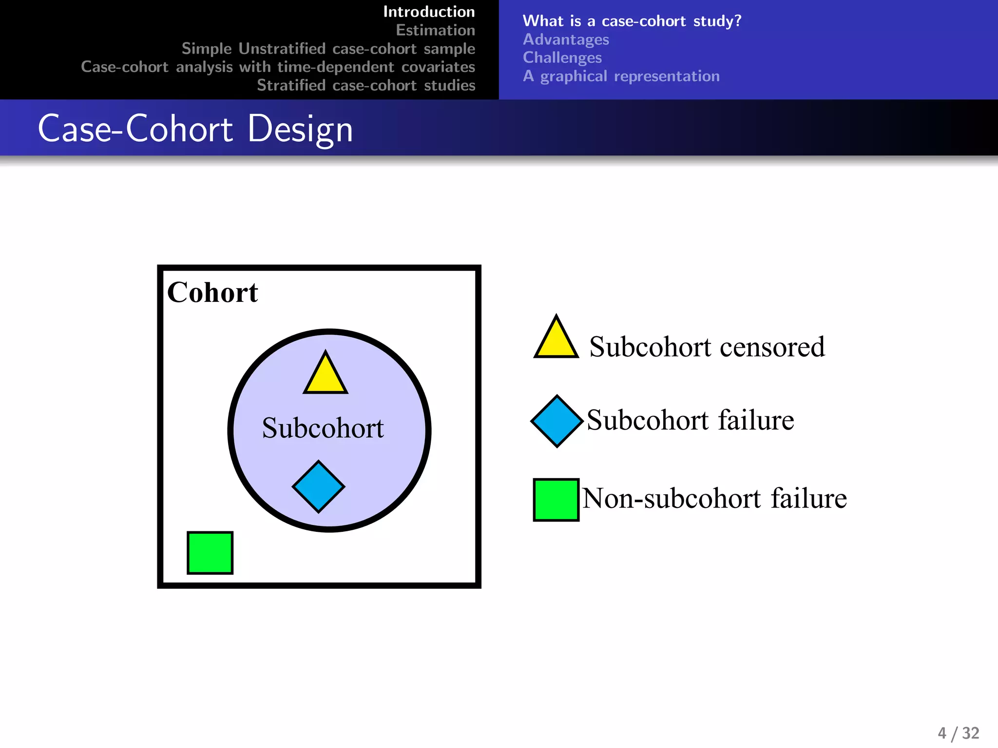
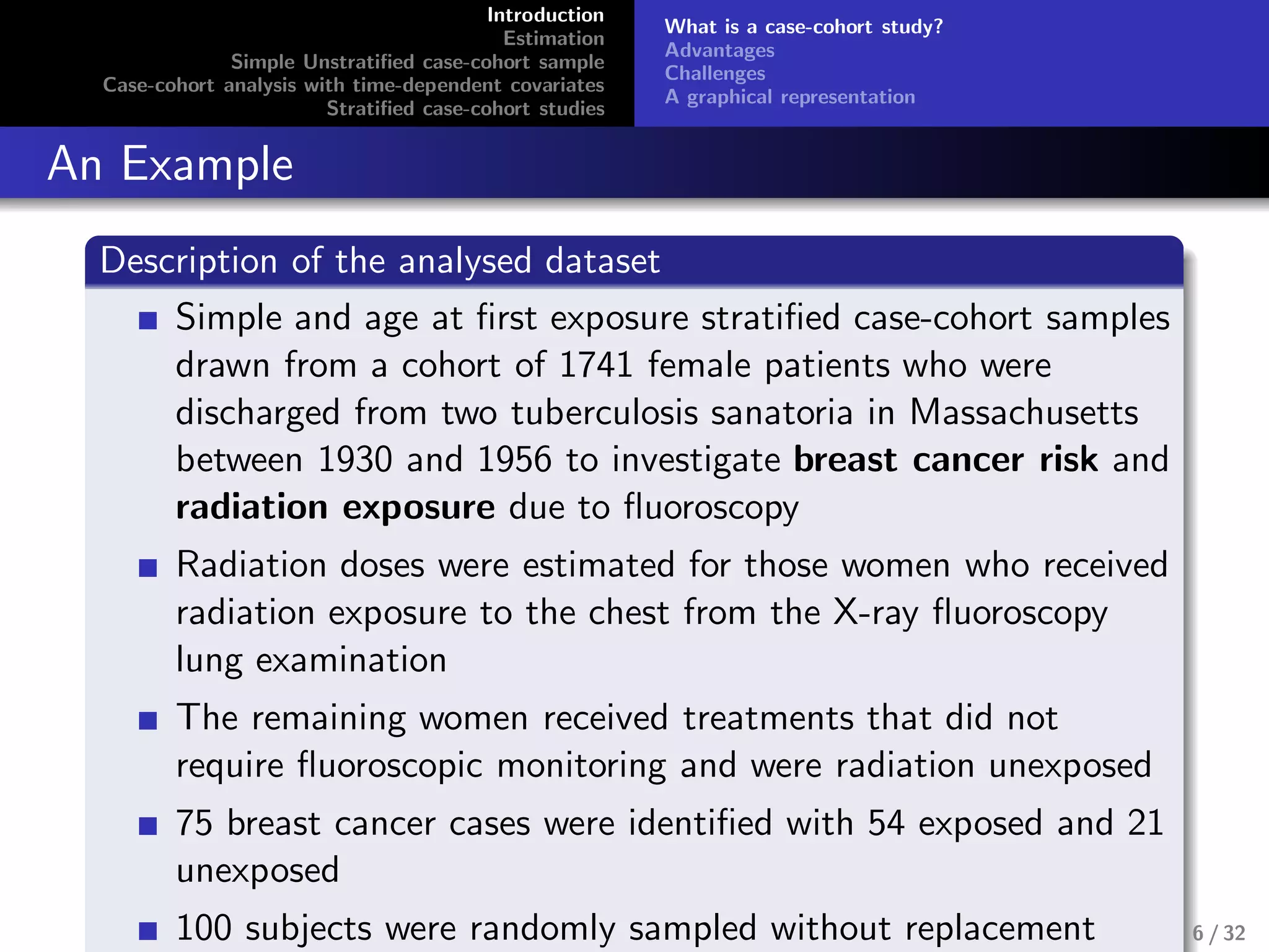
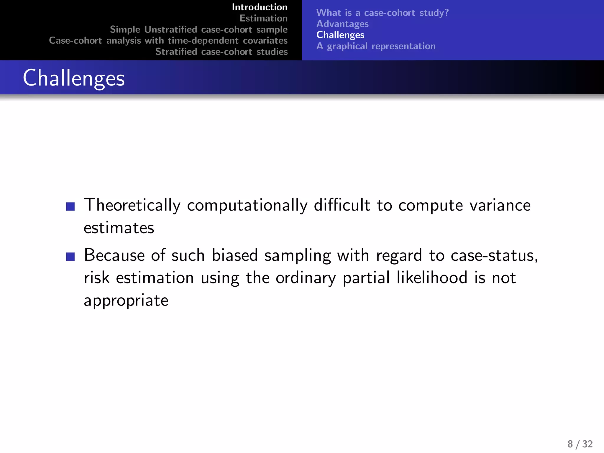
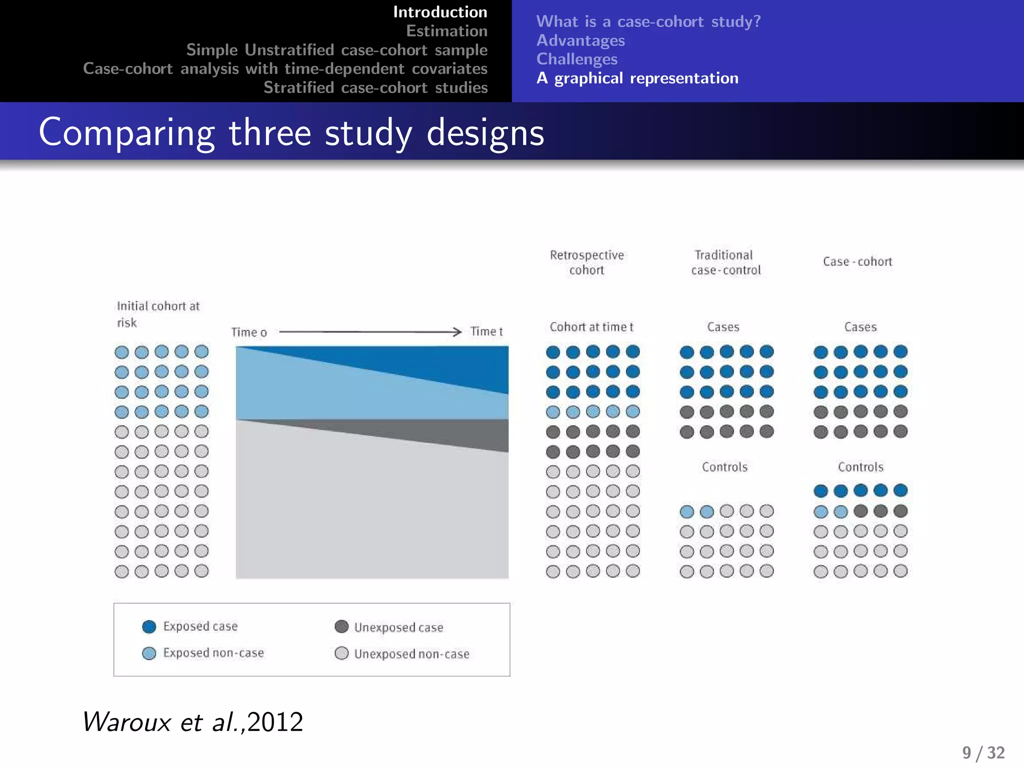
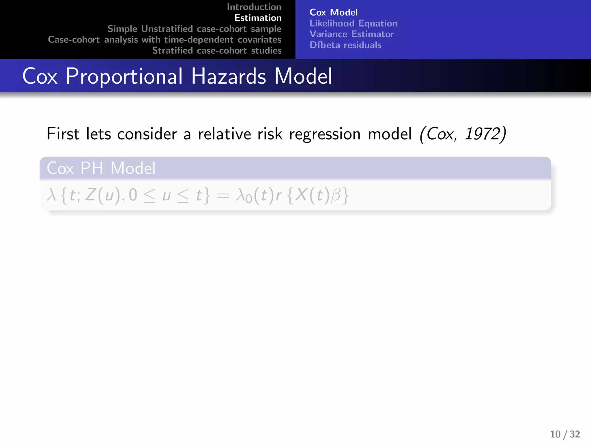
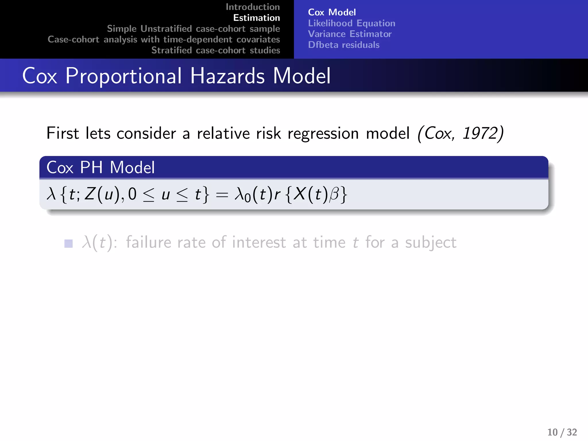
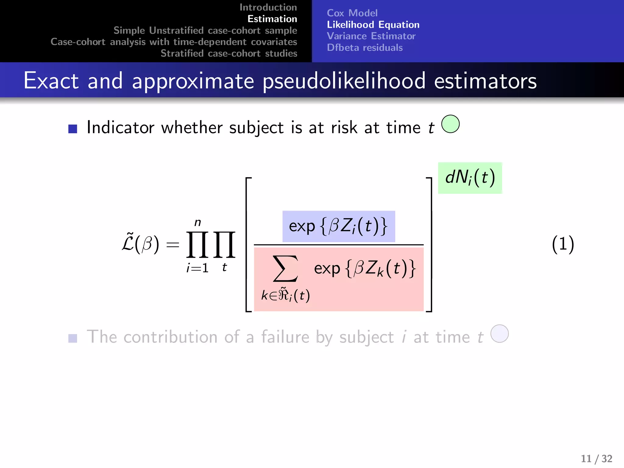
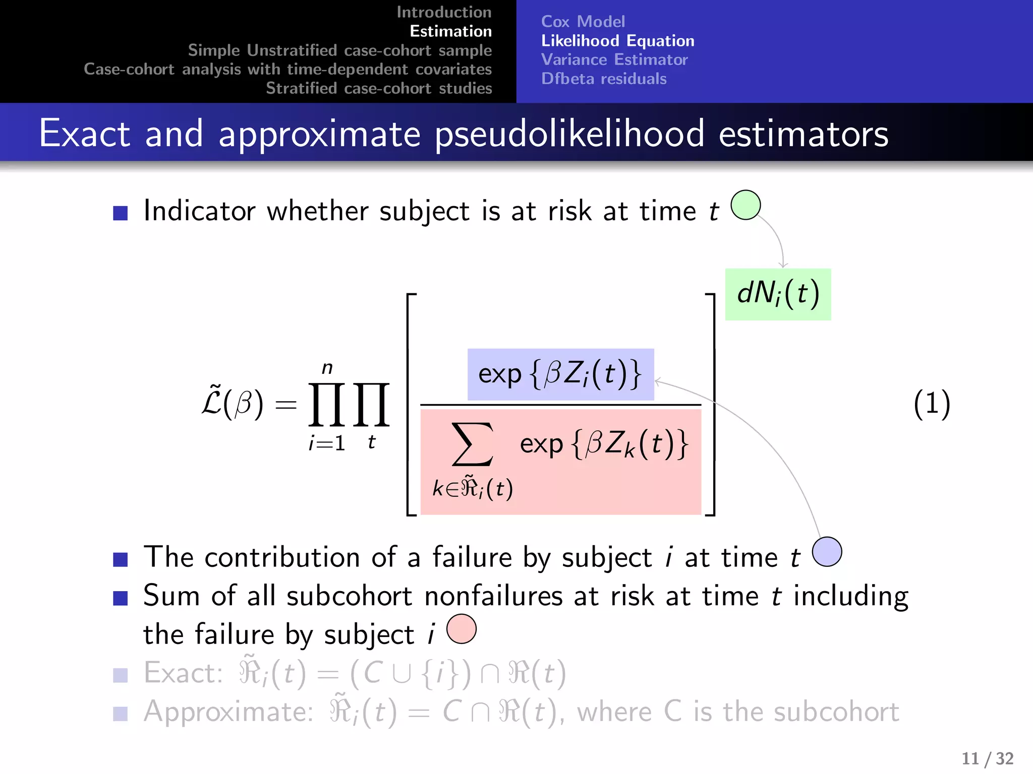
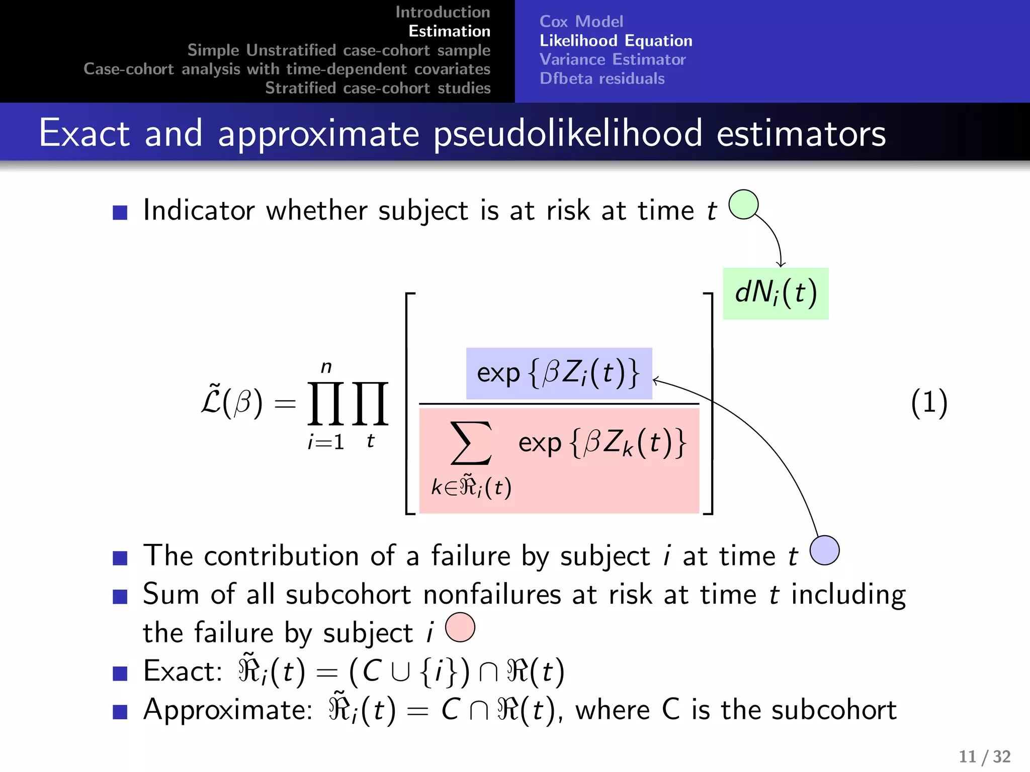
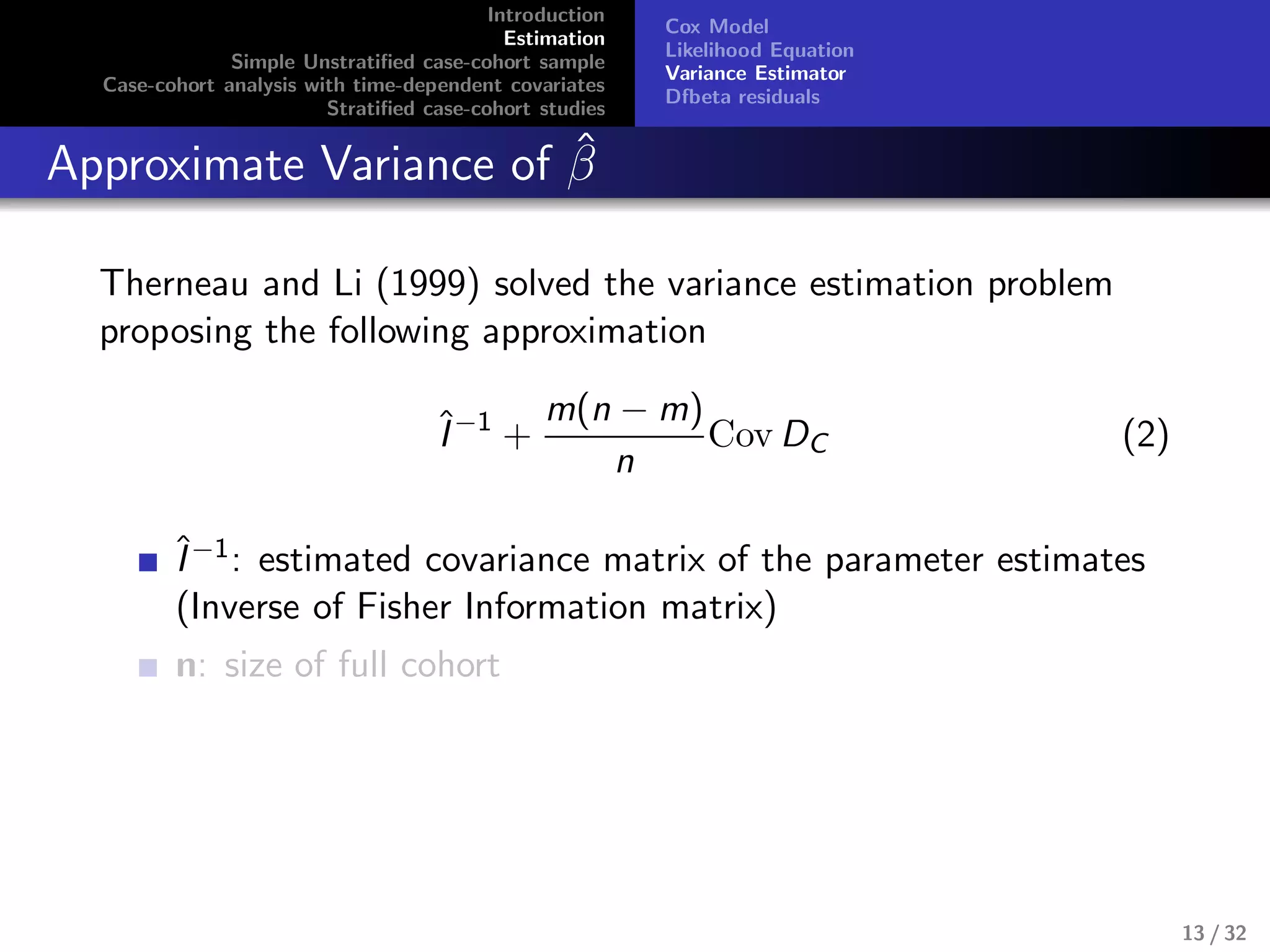
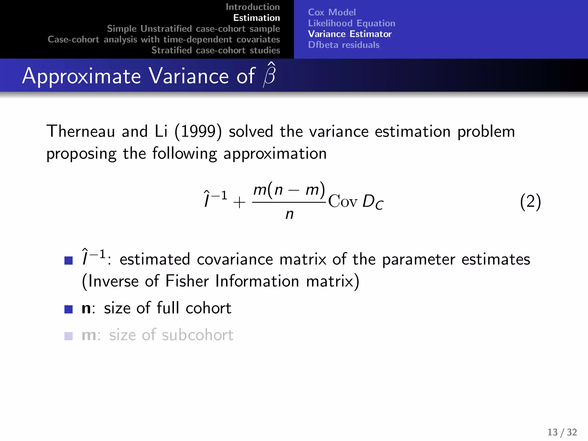
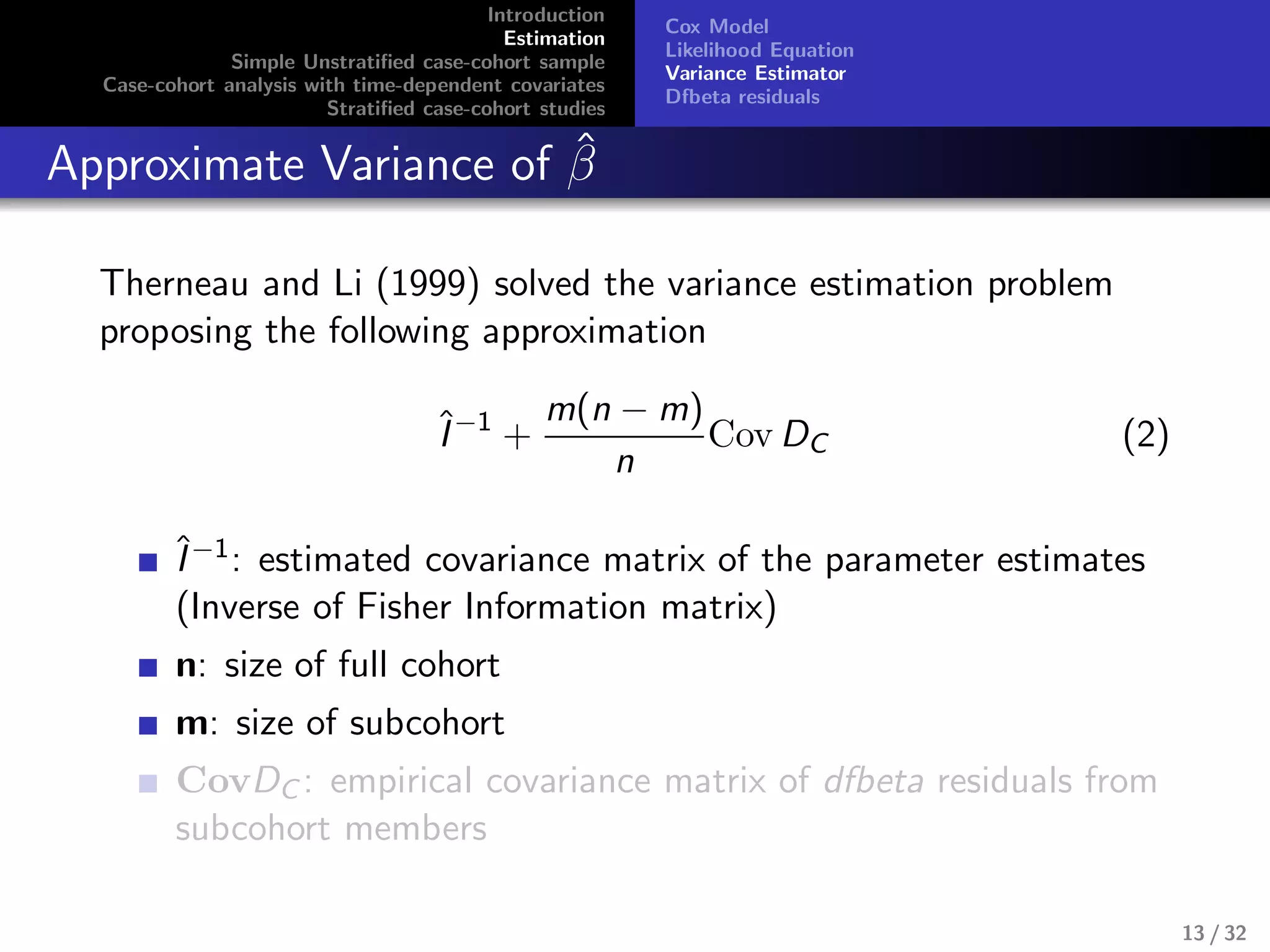
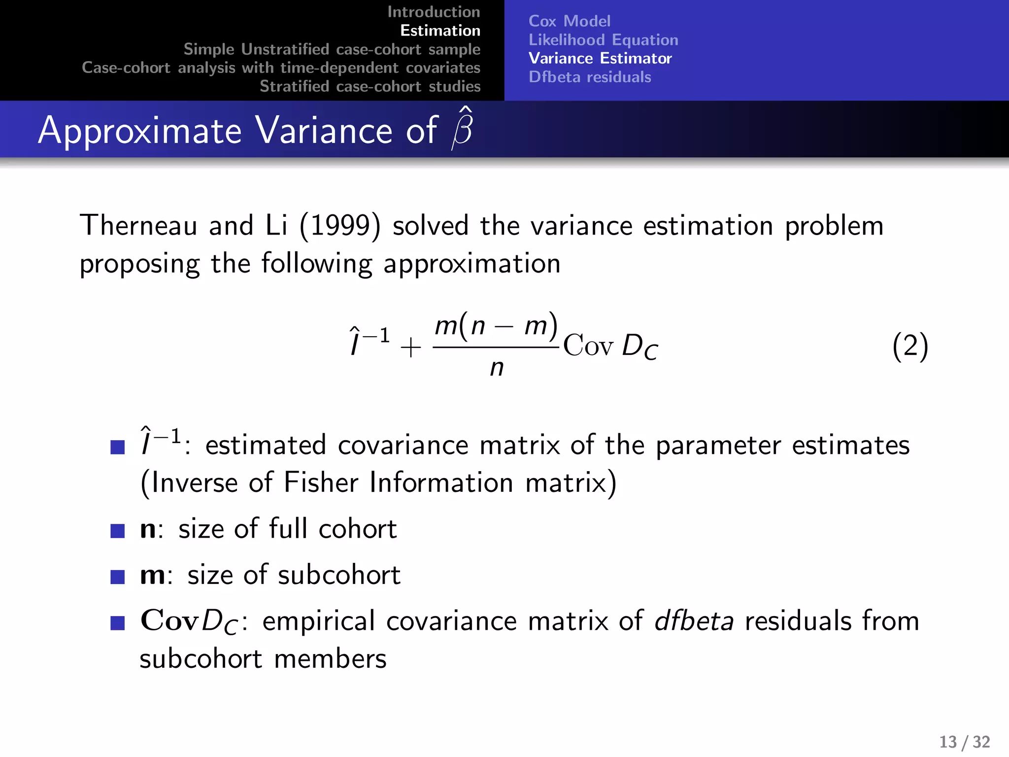
SlideShare a Scribd company logo
1 of 78
Download to read offline
Introduction
Estimation
Simple Unstratified case-cohort sample
Case-cohort analysis with time-dependent covariates
Stratified case-cohort studies
Computational Methods For Case-Cohort Studies
Sahir Rai Bhatnagar
Queen’s University
November 27, 2012
1 / 32
Introduction
Estimation
Simple Unstratified case-cohort sample
Case-cohort analysis with time-dependent covariates
Stratified case-cohort studies
What is a case-cohort study?
Advantages
Challenges
A graphical representation
Cohort studies
All participants provide a wide range of information at time of
recruitment e.g. detailed dietary questionnaires and blood and
urine samples
Because of large numbers and cost of analysing the biological
specimens or genotyping, these resources are often not
analysed in detail at the time but are stored for future use
This design is expensive, inefficient for rare outcomes, long
follow-up period needed, large sample size needed
2 / 32
Introduction
Estimation
Simple Unstratified case-cohort sample
Case-cohort analysis with time-dependent covariates
Stratified case-cohort studies
What is a case-cohort study?
Advantages
Challenges
A graphical representation
Case-Cohort: A more efficient design
A random sample of participants are selected from full cohort
at baseline
Detailed exposure information (covariates) can then be
retrieved for
3 / 32
Introduction
Estimation
Simple Unstratified case-cohort sample
Case-cohort analysis with time-dependent covariates
Stratified case-cohort studies
What is a case-cohort study?
Advantages
Challenges
A graphical representation
Case-Cohort: A more efficient design
A random sample of participants are selected from full cohort
at baseline
Detailed exposure information (covariates) can then be
retrieved for
this subcohort
everyone in the full cohort who develop the disease of interest
Key feature: inclusion of all cases that occur in the cohort
3 / 32
Introduction
Estimation
Simple Unstratified case-cohort sample
Case-cohort analysis with time-dependent covariates
Stratified case-cohort studies
What is a case-cohort study?
Advantages
Challenges
A graphical representation
Case-Cohort Design
Cohort
Subcohort
Subcohort censored
Subcohort failure
Non-subcohort failure
4 / 32
Introduction
Estimation
Simple Unstratified case-cohort sample
Case-cohort analysis with time-dependent covariates
Stratified case-cohort studies
What is a case-cohort study?
Advantages
Challenges
A graphical representation
Objective
Purpose of this presentation
1 Explain and promote the case-cohort design
2 Show that it’s not as difficult as the literature says to
compute accurate estimates
5 / 32
Introduction
Estimation
Simple Unstratified case-cohort sample
Case-cohort analysis with time-dependent covariates
Stratified case-cohort studies
What is a case-cohort study?
Advantages
Challenges
A graphical representation
An Example
Description of the analysed dataset
Simple and age at first exposure stratified case-cohort samples
drawn from a cohort of 1741 female patients who were
discharged from two tuberculosis sanatoria in Massachusetts
between 1930 and 1956 to investigate breast cancer risk and
radiation exposure due to fluoroscopy
6 / 32
Introduction
Estimation
Simple Unstratified case-cohort sample
Case-cohort analysis with time-dependent covariates
Stratified case-cohort studies
What is a case-cohort study?
Advantages
Challenges
A graphical representation
An Example
Description of the analysed dataset
Simple and age at first exposure stratified case-cohort samples
drawn from a cohort of 1741 female patients who were
discharged from two tuberculosis sanatoria in Massachusetts
between 1930 and 1956 to investigate breast cancer risk and
radiation exposure due to fluoroscopy
Radiation doses were estimated for those women who received
radiation exposure to the chest from the X-ray fluoroscopy
lung examination
The remaining women received treatments that did not
require fluoroscopic monitoring and were radiation unexposed
75 breast cancer cases were identified with 54 exposed and 21
unexposed
100 subjects were randomly sampled without replacement 6 / 32
Introduction
Estimation
Simple Unstratified case-cohort sample
Case-cohort analysis with time-dependent covariates
Stratified case-cohort studies
What is a case-cohort study?
Advantages
Challenges
A graphical representation
Advantages
Exposure precedes outcome, while smaller scale reduces cost
and effort
In outbreak situations, multiple outcomes can be studied using
only one sample of controls
7 / 32
Introduction
Estimation
Simple Unstratified case-cohort sample
Case-cohort analysis with time-dependent covariates
Stratified case-cohort studies
What is a case-cohort study?
Advantages
Challenges
A graphical representation
Challenges
Theoretically computationally difficult to compute variance
estimates
Because of such biased sampling with regard to case-status,
risk estimation using the ordinary partial likelihood is not
appropriate
8 / 32
Introduction
Estimation
Simple Unstratified case-cohort sample
Case-cohort analysis with time-dependent covariates
Stratified case-cohort studies
What is a case-cohort study?
Advantages
Challenges
A graphical representation
Comparing three study designs
Waroux et al.,2012
9 / 32
Introduction
Estimation
Simple Unstratified case-cohort sample
Case-cohort analysis with time-dependent covariates
Stratified case-cohort studies
Cox Model
Likelihood Equation
Variance Estimator
Dfbeta residuals
Cox Proportional Hazards Model
First lets consider a relative risk regression model (Cox, 1972)
Cox PH Model
λ {t; Z(u), 0 ≤ u ≤ t} = λ0(t)r {X(t)β}
10 / 32
Introduction
Estimation
Simple Unstratified case-cohort sample
Case-cohort analysis with time-dependent covariates
Stratified case-cohort studies
Cox Model
Likelihood Equation
Variance Estimator
Dfbeta residuals
Cox Proportional Hazards Model
First lets consider a relative risk regression model (Cox, 1972)
Cox PH Model
λ {t; Z(u), 0 ≤ u ≤ t} = λ0(t)r {X(t)β}
λ(t): failure rate of interest at time t for a subject
{Z(u); 0 ≤ u < t}:preceding covariate history
r(x): is a fixed function with r(0) = 1 e.g. r(x) = exp {x}
X(t): row p-vector consisting of functions of Z(u)
β: column p-vector of regression parameters to be estimated
λ0(t): baseline hazard function
10 / 32
Introduction
Estimation
Simple Unstratified case-cohort sample
Case-cohort analysis with time-dependent covariates
Stratified case-cohort studies
Cox Model
Likelihood Equation
Variance Estimator
Dfbeta residuals
Exact and approximate pseudolikelihood estimators
Indicator whether subject is at risk at time t
˜L(β) =
n
i=1 t








exp {βZi (t)}
k∈˜ℜi (t)
exp {βZk(t)}








dNi (t)
(1)
The contribution of a failure by subject i at time t
11 / 32
Introduction
Estimation
Simple Unstratified case-cohort sample
Case-cohort analysis with time-dependent covariates
Stratified case-cohort studies
Cox Model
Likelihood Equation
Variance Estimator
Dfbeta residuals
Exact and approximate pseudolikelihood estimators
Indicator whether subject is at risk at time t
˜L(β) =
n
i=1 t








exp {βZi (t)}
k∈˜ℜi (t)
exp {βZk(t)}








dNi (t)
(1)
The contribution of a failure by subject i at time t
Sum of all subcohort nonfailures at risk at time t including
the failure by subject i
Exact: ˜ℜi (t) = (C ∪ {i}) ∩ ℜ(t)
Approximate: ˜ℜi (t) = C ∩ ℜ(t), where C is the subcohort
11 / 32
Introduction
Estimation
Simple Unstratified case-cohort sample
Case-cohort analysis with time-dependent covariates
Stratified case-cohort studies
Cox Model
Likelihood Equation
Variance Estimator
Dfbeta residuals
Exact and approximate pseudolikelihood estimators
The unique sampling approach i.e. over selecting cases, leads
to a pseudolikelihood rather than the usual partial likelihood
Analysis must adjust for bias introduced in the distributions of
covariates used in calculating the denominator of the
pseudolikelihood
12 / 32
Introduction
Estimation
Simple Unstratified case-cohort sample
Case-cohort analysis with time-dependent covariates
Stratified case-cohort studies
Cox Model
Likelihood Equation
Variance Estimator
Dfbeta residuals
Exact and approximate pseudolikelihood estimators
The unique sampling approach i.e. over selecting cases, leads
to a pseudolikelihood rather than the usual partial likelihood
Analysis must adjust for bias introduced in the distributions of
covariates used in calculating the denominator of the
pseudolikelihood
Bias incurred by including cases outside the subcohort is
corrected by not allowing those cases to contribute to risk sets
other than their own
We will focus our attention the exact approach rather than
the approximate
12 / 32
Introduction
Estimation
Simple Unstratified case-cohort sample
Case-cohort analysis with time-dependent covariates
Stratified case-cohort studies
Cox Model
Likelihood Equation
Variance Estimator
Dfbeta residuals
Approximate Variance of ˆβ
Therneau and Li (1999) solved the variance estimation problem
proposing the following approximation
ˆI−1
+
m(n − m)
n
Cov DC (2)
ˆI−1: estimated covariance matrix of the parameter estimates
(Inverse of Fisher Information matrix)
13 / 32
Introduction
Estimation
Simple Unstratified case-cohort sample
Case-cohort analysis with time-dependent covariates
Stratified case-cohort studies
Cox Model
Likelihood Equation
Variance Estimator
Dfbeta residuals
Approximate Variance of ˆβ
Therneau and Li (1999) solved the variance estimation problem
proposing the following approximation
ˆI−1
+
m(n − m)
n
Cov DC (2)
ˆI−1: estimated covariance matrix of the parameter estimates
(Inverse of Fisher Information matrix)
n: size of full cohort
m: size of subcohort
CovDC : empirical covariance matrix of dfbeta residuals from
subcohort members
13 / 32
Introduction
Estimation
Simple Unstratified case-cohort sample
Case-cohort analysis with time-dependent covariates
Stratified case-cohort studies
Cox Model
Likelihood Equation
Variance Estimator
Dfbeta residuals
Dfbeta residuals
Are the approximate changes in the parameter estimates (ˆβ − ˆβ(j))
when the jth observation is omitted. These variables are a
weighted transform of the score residual variables and are useful in
assessing local influence and in computing approximate and robust
variance estimates.
14 / 32
Introduction
Estimation
Simple Unstratified case-cohort sample
Case-cohort analysis with time-dependent covariates
Stratified case-cohort studies
Creating an analytic dataset
Model output and results
Procedure for creating analytic dataset
Steps
1 Each subcohort non-failure contributes one line of data to the
analytic data set as censored observations
15 / 32
Introduction
Estimation
Simple Unstratified case-cohort sample
Case-cohort analysis with time-dependent covariates
Stratified case-cohort studies
Creating an analytic dataset
Model output and results
Procedure for creating analytic dataset
Steps
1 Each subcohort non-failure contributes one line of data to the
analytic data set as censored observations
2 A non-subcohort failure contributes no information prior to
the failure time so one line of data is contributed to the
analytic data set as a failure but only at the failure time
3 A subcohort failure contributes two lines to the analytic data
set:
one line as a censored observation prior to the failure time
and one line as a failure at the failure time
4 To create a time just before the exit time, an amount less
than the precision of exit times given in the data is subtracted
off from the actual failure time
15 / 32
Introduction
Estimation
Simple Unstratified case-cohort sample
Case-cohort analysis with time-dependent covariates
Stratified case-cohort studies
Creating an analytic dataset
Model output and results
Graphic of how to create analytic dataset
Cohort
t = 0
n
Subcohort censored
Subcohort failure
Non-subcohort failure
anna
lucy
entry exit
entry exit
anna
Legend
n-dt
lucy
entry exit
lucy
16 / 32
Introduction
Estimation
Simple Unstratified case-cohort sample
Case-cohort analysis with time-dependent covariates
Stratified case-cohort studies
Creating an analytic dataset
Model output and results
Original Case Cohort dataset
Basic case-cohort data
Subject
ID
Dose in
rad
Age at exit
(in years)
Age at entry
(in years)
0-cens,1-subc fail
2-non-subc fail
1-249
rad
250+
rad
age at first
exposure group a
2866 0.4525 71.269 34.0014 0 1 0 3
2787 0.00984 69.0294 31.7454 0 1 0 4
2702 0.05486 47.5948 36.5065 0 1 0 3
34 0 55.4387 14.9377 1 0 0 1
3064 0.12788 35.4825 25.6838 0 1 0 3
2766 1.62311 64.3559 30.5161 0 1 0 3
2344 1.0624 69.692 25.4127 0 1 0 3
...
...
...
...
...
...
...
...
2698 0 42.3682 36.2026 2 0 0 4
2577 1.00338 50.9979 26.412 2 1 0 3
2348 1.30725 42.1246 24.1259 2 1 0 3
3106 0 55.2635 27.2635 2 0 0 3
2687 0 47.7563 23.2553 2 0 0 3
3018 1.6723 50.0014 38.8337 2 1 0 4
a
1 :< 15, 2 : 15 − 19, 3 : 20 − 29, 4 : 30+
17 / 32
Introduction
Estimation
Simple Unstratified case-cohort sample
Case-cohort analysis with time-dependent covariates
Stratified case-cohort studies
Creating an analytic dataset
Model output and results
Comparison
Original vs. Analytic dataset
Subject
ID
Dose in
rad
Age at exit
(in years)
Age at entry
(in years)
0-cens,1-subc fail
2-non-subc fail
1-249
rad
250+
rad
age at first
exposure group
an entry an exit an ind
34 0 55.4387 14.9377 1 0 0 1
2344 1.0624 69.692 25.4127 0 1 0 3
2687 0 47.7563 23.2553 2 0 0 3
34 0 55.4387 14.9377 1 0 0 1 14.9377 55.4386 0
34 0 55.4387 14.9377 1 0 0 1 55.4386 55.4387 1
2344 1.0624 69.692 25.4127 0 1 0 3 25.4127 69.6919 0
2687 0 47.7563 23.2553 2 0 0 3 47.7562 47.7563 1
18 / 32
Introduction
Estimation
Simple Unstratified case-cohort sample
Case-cohort analysis with time-dependent covariates
Stratified case-cohort studies
Creating an analytic dataset
Model output and results
SAS Code
proc phreg data=analytic;
model an_exit*an_ind(0) = dcat1 dcat2 /
entry=an_entry covb;
output out=dfbetas dfbeta= dfb_dcat1 dfb_dcat2;
id id;
run;
proc corr data=dfbetas cov;
var dfb_dcat1 dfb_dcat2;
where an_ind eq 0;
run;
covb: outputs the inverse information matrix ˆI−1
cov: outputs the covariance matrix of dfbeta residuals from
subcohort members (WHERE an ind = 0)
19 / 32
Exact pseudolikelihood and Asymptotic variance
Analysis of Maximum Likelihood Estimates
Parameter DF
Parameter
Estimate
Standard
Error
χ2 Pr> χ2 Hazard
Ratio
Label
dcat1 1 0.6572 0.26117 6.332 0.0119 1.929 1-249 rad
dcat2 1 1.55325 0.50118 9.6051 0.0019 4.727 250+ rad
Estimated Covariance Matrix (×10−2)
Parameter dcat1 dcat2
dcat1 1-249 rad 6.821 4.743
dcat2 250+ rad 4.743 25.118
Estimated Covariance Matrix of the dfbeta residuals (×10−4)
Parameter dfb dcat1 dfb dcat2
dfb dcat1 difference in the parameter for dcat1 5.487 2.998
dfb dcat2 difference in the parameter for dcat2 2.998 47.878
Introduction
Estimation
Simple Unstratified case-cohort sample
Case-cohort analysis with time-dependent covariates
Stratified case-cohort studies
Motivation
Manipulating the Data
Model output and results
Time-dependent covariates
The partial likelihood of Cox also allows time-dependent
explanatory variables
An explanatory variable is time-dependent if its value for any
given individual can change over time
21 / 32
Introduction
Estimation
Simple Unstratified case-cohort sample
Case-cohort analysis with time-dependent covariates
Stratified case-cohort studies
Motivation
Manipulating the Data
Model output and results
Time-dependent covariates
The partial likelihood of Cox also allows time-dependent
explanatory variables
An explanatory variable is time-dependent if its value for any
given individual can change over time
We introduce a latency variable lat15 indicating 15 years
since last fluoroscopy
21 / 32
Introduction
Estimation
Simple Unstratified case-cohort sample
Case-cohort analysis with time-dependent covariates
Stratified case-cohort studies
Motivation
Manipulating the Data
Model output and results
Difficulties in programming
Most software can account for time-dependent covariates for
rate ratio estimation, however none can compute dfbeta
residuals for these time-dependent covariates
Thus it is not possible to compute the robust or asymptotic
variance estimators for case-cohort data
22 / 32
Introduction
Estimation
Simple Unstratified case-cohort sample
Case-cohort analysis with time-dependent covariates
Stratified case-cohort studies
Motivation
Manipulating the Data
Model output and results
Proposed solution
Software can be “tricked” to accommodate time-dependent
covariates by organizing the case-cohort data into risk sets
Has the structure of individually matched case-control data
with a risk set formed at each failure time
23 / 32
Introduction
Estimation
Simple Unstratified case-cohort sample
Case-cohort analysis with time-dependent covariates
Stratified case-cohort studies
Motivation
Manipulating the Data
Model output and results
Proposed solution
Software can be “tricked” to accommodate time-dependent
covariates by organizing the case-cohort data into risk sets
Has the structure of individually matched case-control data
with a risk set formed at each failure time
Case: is the failure at a specific failure time
Controls: are all those still at risk at the case failure time
23 / 32
Introduction
Estimation
Simple Unstratified case-cohort sample
Case-cohort analysis with time-dependent covariates
Stratified case-cohort studies
Motivation
Manipulating the Data
Model output and results
Analytic dataset
Analytic Dataset for time dependent covariates
Caseid set no rstime rsentry
Subject
ID
Dose in
rad
Age at exit
(in years)
Age at entry
(in years)
0-cens,1-subc fail
2-non-subc fail
1-249
rad
250+
rad
age at first
exposure group
ccohentry cc latency lat15
22 1 25.4292 25.4291 22 0.61714 25.4292 17.1773 1 1 0 1 17.1773 1 8.2519 0
22 1 25.4292 25.4291 2958 4.13045 33.6016 15.8303 0 0 1 1 15.8303 0 9.5989 0
22 1 25.4292 25.4291 295 0.58148 51.833 17.5496 0 1 0 2 17.5496 0 7.8795 0
22 1 25.4292 25.4291 261 0 52.8569 3.4771 0 0 0 1 3.4771 0 21.9521 1
...
...
...
...
...
...
...
...
...
...
...
...
...
...
...
...
22 1 25.4292 25.4291 34 0 55.4387 14.9377 1 0 0 1 14.9377 0 10.4914 0
22 1 25.4292 25.4291 334 1.15677 56.6543 18.3381 0 1 0 2 18.3381 0 7.091 0
22 1 25.4292 25.4291 2057 0 73.2402 20.8049 0 0 0 2 20.8049 0 4.6242 0
2350 33 47.7235 47.7234 2350 0.94436 47.7235 20.2218 2 1 0 2 47.7234 1 27.5017 1
2350 33 47.7235 47.7234 3043 0.92604 48.909 17.5414 0 1 0 1 17.5414 0 30.1821 1
2350 33 47.7235 47.7234 242 0.67137 49.1608 15.8795 0 1 0 1 15.8795 0 31.8439 1
2350 33 47.7235 47.7234 2244 0.00959 49.1828 16.9035 0 1 0 2 16.9035 0 30.82 1
2350 33 47.7235 47.7234 3150 0 50.4723 17.191 0 0 0 2 17.191 0 30.5325 1
...
...
...
...
...
...
...
...
...
...
...
...
...
...
...
...
2350 33 47.7235 47.7234 3317 1.28865 78.4559 27.7755 0 1 0 3 27.7755 0 19.948 1
2350 33 47.7235 47.7234 3182 0.95419 81.0951 35.05 0 1 0 4 35.05 0 12.6735 0
2350 33 47.7235 47.7234 3258 0.82631 86.642 38.36 0 1 0 4 38.36 0 9.3634 0
2350 33 47.7235 47.7234 3198 0 87.1157 42.5435 0 0 0 4 42.5435 0 5.18 0
3085 75 77.86 77.86 3085 0 77.8645 43.0335 2 0 0 4 77.8644 1 34.83 1
3085 75 77.86 77.86 3317 1.28865 78.4559 27.7755 0 1 0 3 27.7755 0 50.09 1
3085 75 77.86 77.86 3182 0.95419 81.0951 35.05 0 1 0 4 35.05 0 42.81 1
3085 75 77.86 77.86 3258 0.82631 86.642 38.36 0 1 0 4 38.36 0 39.5 1
3085 75 77.86 77.86 3198 0 87.1157 42.5435 0 0 0 4 42.5435 0 35.32 1
3085 75 77.86 77.86 2477 0 89.9849 53.9001 0 0 0 4 53.9001 0 23.96 1
24 / 32
Introduction
Estimation
Simple Unstratified case-cohort sample
Case-cohort analysis with time-dependent covariates
Stratified case-cohort studies
Motivation
Manipulating the Data
Model output and results
SAS Code
proc phreg data=pclib.td_analytic nosummary;
model rstime*cc(0) = dcat1 dcat2 lat15
/ entry=rsentry covb;
output out=dfbetas dfbeta= dfb_dcat1 dfb_dcat2 dfb_lat15;
id id;
run;
proc summary data=dfbetas sum;
class id;
var dfb_dcat1 dfb_dcat2 dfb_lat15;
output out=summed sum=dfb_dcat1 dfb_dcat2 dfb_lat15;
where cc eq 0;
run;
proc corr data=summed cov;
var dfb_dcat1 dfb_dcat2 dfb_lat15;
run;
25 / 32
Introduction
Estimation
Simple Unstratified case-cohort sample
Case-cohort analysis with time-dependent covariates
Stratified case-cohort studies
Motivation
Manipulating the Data
Model output and results
Exact pseudolikelihood estimators
Analysis of Maximum Likelihood Estimates
Parameter DF
Parameter
Estimate
Standard
Error
χ2 Pr> χ2 Hazard
Ratio
Label
dcat1 1 0.65709 0.26112 6.3325 0.0119 1.929 1-249 rad
dcat2 1 1.68786 0.50750 11.0610 0.0009 4.727 250+ rad
lat15 1 0.61486 0.36062 2.9071 0.0882 1.849
26 / 32
Introduction
Estimation
Simple Unstratified case-cohort sample
Case-cohort analysis with time-dependent covariates
Stratified case-cohort studies
Confounder stratified case-cohort study
SAS Code
Results: Stratified vs. Unstratified
Summary
References
Stratification by age at first exposure
It is quite possible that age is confounding the main effects of
the covariates
To control for confounding we stratify by age at first exposure
group
Each stratum (s) contributes independently to the
pseudolikelihood
the asymptotic variance is given by
ˆI−1
+
s
ms(ns − ms )
ns
Cov DCs (3)
27 / 32
Introduction
Estimation
Simple Unstratified case-cohort sample
Case-cohort analysis with time-dependent covariates
Stratified case-cohort studies
Confounder stratified case-cohort study
SAS Code
Results: Stratified vs. Unstratified
Summary
References
Stratification
Age Stratified Groups
Age Group number
<15 1
15-19 2
20-29 3
30+ 4
27 / 32
Introduction
Estimation
Simple Unstratified case-cohort sample
Case-cohort analysis with time-dependent covariates
Stratified case-cohort studies
Confounder stratified case-cohort study
SAS Code
Results: Stratified vs. Unstratified
Summary
References
SAS Code
proc phreg data=analytic;
model an_exit*an_ind(0) = dcat1 dcat2 / entry=an_entry covb;
output out=dfbetas dfbeta= dfb_dcat1 dfb_dcat2;
strata agefirstgr;
id id;
run;
proc corr data=dfbetas cov;
var dfb_dcat1 dfb_dcat2;
by agefirstgr;
where an_ind eq 0;
run;
28 / 32
Exact pseudolikelihood estimators
Stratified
Analysis of Maximum Likelihood Estimates
Parameter DF
Parameter
Estimate
Standard
Error
χ2 Pr> χ2 Hazard
Ratio
Label
dcat1 1 0.5938 0.27148 4.7838 0.0287 1.811 1-249 rad
dcat2 1 0.9349 0.51737 3.2655 0.0708 2.547 250+ rad
Unstratified
Analysis of Maximum Likelihood Estimates
Parameter DF
Parameter
Estimate
Standard
Error
χ2 Pr> χ2 Hazard
Ratio
Label
dcat1 1 0.6572 0.26117 6.332 0.0119 1.929 1-249 rad
dcat2 1 1.55325 0.50118 9.6051 0.0019 4.727 250+ rad
Introduction
Estimation
Simple Unstratified case-cohort sample
Case-cohort analysis with time-dependent covariates
Stratified case-cohort studies
Confounder stratified case-cohort study
SAS Code
Results: Stratified vs. Unstratified
Summary
References
Summary
1 Efficiency and benefits of case-cohort design
2 Take advantage of available software
30 / 32
Introduction
Estimation
Simple Unstratified case-cohort sample
Case-cohort analysis with time-dependent covariates
Stratified case-cohort studies
Confounder stratified case-cohort study
SAS Code
Results: Stratified vs. Unstratified
Summary
References
References I
Bryan Langholz and Jenny Jiao
Computational methods for case cohort studies
Computational Statistics & Data Analysis, 51:2007
J. Cologne et al.
Conventional case-cohort design and analysis for studies of
interaction
International Journal of Epidemiology, 41:2012
Therneau, T and Li, H
Computing the Cox model for case cohort designs
Lifetime data analysis, 2(5):1999
31 / 32
Introduction
Estimation
Simple Unstratified case-cohort sample
Case-cohort analysis with time-dependent covariates
Stratified case-cohort studies
Confounder stratified case-cohort study
SAS Code
Results: Stratified vs. Unstratified
Summary
References
References II
Penny Webb and Chris Bain.
Essential Epidemiology.
Cambridge University Press, 2nd edition, 2011.
O Le Polain de Waroux
The case-cohort design in outbreak investigations
Euro surveillance, 17(25):2012
32 / 32

More Related Content

What's hot

What's hot (20)

COHORT STUDY
COHORT STUDY COHORT STUDY
COHORT STUDY
 
Cohort study
Cohort studyCohort study
Cohort study
 
Nested case control study
Nested case control studyNested case control study
Nested case control study
 
EPIDEMIOLOGICAL RESEARCH DESIGN
EPIDEMIOLOGICAL RESEARCH DESIGNEPIDEMIOLOGICAL RESEARCH DESIGN
EPIDEMIOLOGICAL RESEARCH DESIGN
 
4. case control study
4. case control study4. case control study
4. case control study
 
Cohort studies
Cohort studiesCohort studies
Cohort studies
 
unmatched case control studies
unmatched case control studiesunmatched case control studies
unmatched case control studies
 
Cohort Study
Cohort Study Cohort Study
Cohort Study
 
Farmacoepi Course Leiden 0210 Part 2
Farmacoepi Course Leiden 0210   Part 2Farmacoepi Course Leiden 0210   Part 2
Farmacoepi Course Leiden 0210 Part 2
 
Cohort study
Cohort studyCohort study
Cohort study
 
7. experimental epidemiology
7. experimental epidemiology7. experimental epidemiology
7. experimental epidemiology
 
5. cohort studies
5. cohort  studies5. cohort  studies
5. cohort studies
 
Cohort Study
Cohort StudyCohort Study
Cohort Study
 
Cohort Studies by Dr. Mohammed Jawad 2020
Cohort Studies by Dr. Mohammed Jawad 2020Cohort Studies by Dr. Mohammed Jawad 2020
Cohort Studies by Dr. Mohammed Jawad 2020
 
Case control studies and cohort studies
Case control studies and cohort studiesCase control studies and cohort studies
Case control studies and cohort studies
 
cohort study
cohort studycohort study
cohort study
 
Steps in cohort study
Steps in cohort studySteps in cohort study
Steps in cohort study
 
Types of clinical studies
Types of clinical studiesTypes of clinical studies
Types of clinical studies
 
Systematic review of master protocols
Systematic review of master protocolsSystematic review of master protocols
Systematic review of master protocols
 
Sample and sample technique
Sample and sample techniqueSample and sample technique
Sample and sample technique
 

Similar to Computational methods for case-cohort studies

Research and methodology 2
Research and methodology 2Research and methodology 2
Research and methodology 2Tosif Ahmad
 
Week 02, Stux f gfgzgzch nxfgnfxndy Designs.pptx
Week 02, Stux f gfgzgzch nxfgnfxndy Designs.pptxWeek 02, Stux f gfgzgzch nxfgnfxndy Designs.pptx
Week 02, Stux f gfgzgzch nxfgnfxndy Designs.pptxsaeedapkli
 
Noncommunicable diseases - descriptive & analytical studies
Noncommunicable diseases - descriptive & analytical studiesNoncommunicable diseases - descriptive & analytical studies
Noncommunicable diseases - descriptive & analytical studiesRizwan S A
 
Overview of Epidemiological Study
Overview of Epidemiological StudyOverview of Epidemiological Study
Overview of Epidemiological StudyUltraman Taro
 
Overview of Diffrent types of studies in clinical research.pptx
Overview of Diffrent types of studies in clinical research.pptxOverview of Diffrent types of studies in clinical research.pptx
Overview of Diffrent types of studies in clinical research.pptxAhmed Elshebiny
 
Types of studies in research
Types of studies in researchTypes of studies in research
Types of studies in researchYashodharaGaur1
 
4 Epidemiological Study Designs 1.pdf
4 Epidemiological Study Designs 1.pdf4 Epidemiological Study Designs 1.pdf
4 Epidemiological Study Designs 1.pdfmergawekwaya
 
Observational Research designs: detailed description
Observational Research designs: detailed description Observational Research designs: detailed description
Observational Research designs: detailed description Tarek Tawfik Amin
 
Study design
Study designStudy design
Study designRSS6
 
Epidemiological methods.pptx
Epidemiological methods.pptxEpidemiological methods.pptx
Epidemiological methods.pptxUrduKahani
 
Nested case control,
Nested case control,Nested case control,
Nested case control,shefali jain
 
3. Health Research Methods.ppt
3. Health Research Methods.ppt3. Health Research Methods.ppt
3. Health Research Methods.pptFerhanKadir
 
Analytical study designs.pptx
Analytical study designs.pptxAnalytical study designs.pptx
Analytical study designs.pptxAryasree L
 
Sampling and its variability
Sampling  and its variabilitySampling  and its variability
Sampling and its variabilityDrBhushan Kamble
 
What is the best evidence in medicine?
What is the best evidence in medicine?What is the best evidence in medicine?
What is the best evidence in medicine?Samir Haffar
 

Similar to Computational methods for case-cohort studies (20)

Research and methodology 2
Research and methodology 2Research and methodology 2
Research and methodology 2
 
Week 02, Stux f gfgzgzch nxfgnfxndy Designs.pptx
Week 02, Stux f gfgzgzch nxfgnfxndy Designs.pptxWeek 02, Stux f gfgzgzch nxfgnfxndy Designs.pptx
Week 02, Stux f gfgzgzch nxfgnfxndy Designs.pptx
 
Noncommunicable diseases - descriptive & analytical studies
Noncommunicable diseases - descriptive & analytical studiesNoncommunicable diseases - descriptive & analytical studies
Noncommunicable diseases - descriptive & analytical studies
 
Overview of Epidemiological Study
Overview of Epidemiological StudyOverview of Epidemiological Study
Overview of Epidemiological Study
 
Overview of Diffrent types of studies in clinical research.pptx
Overview of Diffrent types of studies in clinical research.pptxOverview of Diffrent types of studies in clinical research.pptx
Overview of Diffrent types of studies in clinical research.pptx
 
Types of studies in research
Types of studies in researchTypes of studies in research
Types of studies in research
 
4 Epidemiological Study Designs 1.pdf
4 Epidemiological Study Designs 1.pdf4 Epidemiological Study Designs 1.pdf
4 Epidemiological Study Designs 1.pdf
 
Research
ResearchResearch
Research
 
Sampling
SamplingSampling
Sampling
 
Observational Research designs: detailed description
Observational Research designs: detailed description Observational Research designs: detailed description
Observational Research designs: detailed description
 
Study design
Study designStudy design
Study design
 
Study design
Study designStudy design
Study design
 
Epidemiological methods.pptx
Epidemiological methods.pptxEpidemiological methods.pptx
Epidemiological methods.pptx
 
Nested case control,
Nested case control,Nested case control,
Nested case control,
 
CT Screening for Lung Cancer
CT Screening for Lung CancerCT Screening for Lung Cancer
CT Screening for Lung Cancer
 
3. Health Research Methods.ppt
3. Health Research Methods.ppt3. Health Research Methods.ppt
3. Health Research Methods.ppt
 
Analytical study designs.pptx
Analytical study designs.pptxAnalytical study designs.pptx
Analytical study designs.pptx
 
Sampling and its variability
Sampling  and its variabilitySampling  and its variability
Sampling and its variability
 
What is the best evidence in medicine?
What is the best evidence in medicine?What is the best evidence in medicine?
What is the best evidence in medicine?
 
3 cross sectional study
3 cross sectional study3 cross sectional study
3 cross sectional study
 

More from sahirbhatnagar

Strong Heredity Models in High Dimensional Data
Strong Heredity Models in High Dimensional DataStrong Heredity Models in High Dimensional Data
Strong Heredity Models in High Dimensional Datasahirbhatnagar
 
Methods for High Dimensional Interactions
Methods for High Dimensional InteractionsMethods for High Dimensional Interactions
Methods for High Dimensional Interactionssahirbhatnagar
 
An introduction to knitr and R Markdown
An introduction to knitr and R MarkdownAn introduction to knitr and R Markdown
An introduction to knitr and R Markdownsahirbhatnagar
 
Reproducible Research: An Introduction to knitr
Reproducible Research: An Introduction to knitrReproducible Research: An Introduction to knitr
Reproducible Research: An Introduction to knitrsahirbhatnagar
 
Analysis of DNA methylation and Gene expression to predict childhood obesity
Analysis of DNA methylation and Gene expression to predict childhood obesityAnalysis of DNA methylation and Gene expression to predict childhood obesity
Analysis of DNA methylation and Gene expression to predict childhood obesitysahirbhatnagar
 
Estimation and Accuracy after Model Selection
Estimation and Accuracy after Model SelectionEstimation and Accuracy after Model Selection
Estimation and Accuracy after Model Selectionsahirbhatnagar
 
Factors influencing participation in cancer screening
Factors influencing participation in cancer screeningFactors influencing participation in cancer screening
Factors influencing participation in cancer screeningsahirbhatnagar
 
Methylation and Expression data integration
Methylation and Expression data integrationMethylation and Expression data integration
Methylation and Expression data integrationsahirbhatnagar
 

More from sahirbhatnagar (11)

Strong Heredity Models in High Dimensional Data
Strong Heredity Models in High Dimensional DataStrong Heredity Models in High Dimensional Data
Strong Heredity Models in High Dimensional Data
 
Methods for High Dimensional Interactions
Methods for High Dimensional InteractionsMethods for High Dimensional Interactions
Methods for High Dimensional Interactions
 
An introduction to knitr and R Markdown
An introduction to knitr and R MarkdownAn introduction to knitr and R Markdown
An introduction to knitr and R Markdown
 
Atelier r-gerad
Atelier r-geradAtelier r-gerad
Atelier r-gerad
 
Reproducible Research: An Introduction to knitr
Reproducible Research: An Introduction to knitrReproducible Research: An Introduction to knitr
Reproducible Research: An Introduction to knitr
 
Analysis of DNA methylation and Gene expression to predict childhood obesity
Analysis of DNA methylation and Gene expression to predict childhood obesityAnalysis of DNA methylation and Gene expression to predict childhood obesity
Analysis of DNA methylation and Gene expression to predict childhood obesity
 
Estimation and Accuracy after Model Selection
Estimation and Accuracy after Model SelectionEstimation and Accuracy after Model Selection
Estimation and Accuracy after Model Selection
 
Factors influencing participation in cancer screening
Factors influencing participation in cancer screeningFactors influencing participation in cancer screening
Factors influencing participation in cancer screening
 
Introduction to LaTeX
Introduction to LaTeXIntroduction to LaTeX
Introduction to LaTeX
 
Methylation and Expression data integration
Methylation and Expression data integrationMethylation and Expression data integration
Methylation and Expression data integration
 
Reproducible Research
Reproducible ResearchReproducible Research
Reproducible Research
 

Recently uploaded

ALL ABOUT MIXTURES IN GRADE 7 CLASS PPTX
ALL ABOUT MIXTURES IN GRADE 7 CLASS PPTXALL ABOUT MIXTURES IN GRADE 7 CLASS PPTX
ALL ABOUT MIXTURES IN GRADE 7 CLASS PPTXDole Philippines School
 
User Guide: Magellan MX™ Weather Station
User Guide: Magellan MX™ Weather StationUser Guide: Magellan MX™ Weather Station
User Guide: Magellan MX™ Weather StationColumbia Weather Systems
 
User Guide: Orion™ Weather Station (Columbia Weather Systems)
User Guide: Orion™ Weather Station (Columbia Weather Systems)User Guide: Orion™ Weather Station (Columbia Weather Systems)
User Guide: Orion™ Weather Station (Columbia Weather Systems)Columbia Weather Systems
 
Pests of Blackgram, greengram, cowpea_Dr.UPR.pdf
Pests of Blackgram, greengram, cowpea_Dr.UPR.pdfPests of Blackgram, greengram, cowpea_Dr.UPR.pdf
Pests of Blackgram, greengram, cowpea_Dr.UPR.pdfPirithiRaju
 
Pests of Bengal gram_Identification_Dr.UPR.pdf
Pests of Bengal gram_Identification_Dr.UPR.pdfPests of Bengal gram_Identification_Dr.UPR.pdf
Pests of Bengal gram_Identification_Dr.UPR.pdfPirithiRaju
 
GENERAL PHYSICS 2 REFRACTION OF LIGHT SENIOR HIGH SCHOOL GENPHYS2.pptx
GENERAL PHYSICS 2 REFRACTION OF LIGHT SENIOR HIGH SCHOOL GENPHYS2.pptxGENERAL PHYSICS 2 REFRACTION OF LIGHT SENIOR HIGH SCHOOL GENPHYS2.pptx
GENERAL PHYSICS 2 REFRACTION OF LIGHT SENIOR HIGH SCHOOL GENPHYS2.pptxRitchAndruAgustin
 
Dubai Calls Girl Lisa O525547819 Lexi Call Girls In Dubai
Dubai Calls Girl Lisa O525547819 Lexi Call Girls In DubaiDubai Calls Girl Lisa O525547819 Lexi Call Girls In Dubai
Dubai Calls Girl Lisa O525547819 Lexi Call Girls In Dubaikojalkojal131
 
Pests of safflower_Binomics_Identification_Dr.UPR.pdf
Pests of safflower_Binomics_Identification_Dr.UPR.pdfPests of safflower_Binomics_Identification_Dr.UPR.pdf
Pests of safflower_Binomics_Identification_Dr.UPR.pdfPirithiRaju
 
《Queensland毕业文凭-昆士兰大学毕业证成绩单》
《Queensland毕业文凭-昆士兰大学毕业证成绩单》《Queensland毕业文凭-昆士兰大学毕业证成绩单》
《Queensland毕业文凭-昆士兰大学毕业证成绩单》rnrncn29
 
User Guide: Pulsar™ Weather Station (Columbia Weather Systems)
User Guide: Pulsar™ Weather Station (Columbia Weather Systems)User Guide: Pulsar™ Weather Station (Columbia Weather Systems)
User Guide: Pulsar™ Weather Station (Columbia Weather Systems)Columbia Weather Systems
 
REVISTA DE BIOLOGIA E CIÊNCIAS DA TERRA ISSN 1519-5228 - Artigo_Bioterra_V24_...
REVISTA DE BIOLOGIA E CIÊNCIAS DA TERRA ISSN 1519-5228 - Artigo_Bioterra_V24_...REVISTA DE BIOLOGIA E CIÊNCIAS DA TERRA ISSN 1519-5228 - Artigo_Bioterra_V24_...
REVISTA DE BIOLOGIA E CIÊNCIAS DA TERRA ISSN 1519-5228 - Artigo_Bioterra_V24_...Universidade Federal de Sergipe - UFS
 
LIGHT-PHENOMENA-BY-CABUALDIONALDOPANOGANCADIENTE-CONDEZA (1).pptx
LIGHT-PHENOMENA-BY-CABUALDIONALDOPANOGANCADIENTE-CONDEZA (1).pptxLIGHT-PHENOMENA-BY-CABUALDIONALDOPANOGANCADIENTE-CONDEZA (1).pptx
LIGHT-PHENOMENA-BY-CABUALDIONALDOPANOGANCADIENTE-CONDEZA (1).pptxmalonesandreagweneth
 
Pests of soyabean_Binomics_IdentificationDr.UPR.pdf
Pests of soyabean_Binomics_IdentificationDr.UPR.pdfPests of soyabean_Binomics_IdentificationDr.UPR.pdf
Pests of soyabean_Binomics_IdentificationDr.UPR.pdfPirithiRaju
 
Microteaching on terms used in filtration .Pharmaceutical Engineering
Microteaching on terms used in filtration .Pharmaceutical EngineeringMicroteaching on terms used in filtration .Pharmaceutical Engineering
Microteaching on terms used in filtration .Pharmaceutical EngineeringPrajakta Shinde
 
GenAI talk for Young at Wageningen University & Research (WUR) March 2024
GenAI talk for Young at Wageningen University & Research (WUR) March 2024GenAI talk for Young at Wageningen University & Research (WUR) March 2024
GenAI talk for Young at Wageningen University & Research (WUR) March 2024Jene van der Heide
 
PROJECTILE MOTION-Horizontal and Vertical
PROJECTILE MOTION-Horizontal and VerticalPROJECTILE MOTION-Horizontal and Vertical
PROJECTILE MOTION-Horizontal and VerticalMAESTRELLAMesa2
 
Best Call Girls In Sector 29 Gurgaon❤️8860477959 EscorTs Service In 24/7 Delh...
Best Call Girls In Sector 29 Gurgaon❤️8860477959 EscorTs Service In 24/7 Delh...Best Call Girls In Sector 29 Gurgaon❤️8860477959 EscorTs Service In 24/7 Delh...
Best Call Girls In Sector 29 Gurgaon❤️8860477959 EscorTs Service In 24/7 Delh...lizamodels9
 
Fertilization: Sperm and the egg—collectively called the gametes—fuse togethe...
Fertilization: Sperm and the egg—collectively called the gametes—fuse togethe...Fertilization: Sperm and the egg—collectively called the gametes—fuse togethe...
Fertilization: Sperm and the egg—collectively called the gametes—fuse togethe...D. B. S. College Kanpur
 
Citronella presentation SlideShare mani upadhyay
Citronella presentation SlideShare mani upadhyayCitronella presentation SlideShare mani upadhyay
Citronella presentation SlideShare mani upadhyayupadhyaymani499
 

Recently uploaded (20)

ALL ABOUT MIXTURES IN GRADE 7 CLASS PPTX
ALL ABOUT MIXTURES IN GRADE 7 CLASS PPTXALL ABOUT MIXTURES IN GRADE 7 CLASS PPTX
ALL ABOUT MIXTURES IN GRADE 7 CLASS PPTX
 
User Guide: Magellan MX™ Weather Station
User Guide: Magellan MX™ Weather StationUser Guide: Magellan MX™ Weather Station
User Guide: Magellan MX™ Weather Station
 
User Guide: Orion™ Weather Station (Columbia Weather Systems)
User Guide: Orion™ Weather Station (Columbia Weather Systems)User Guide: Orion™ Weather Station (Columbia Weather Systems)
User Guide: Orion™ Weather Station (Columbia Weather Systems)
 
Pests of Blackgram, greengram, cowpea_Dr.UPR.pdf
Pests of Blackgram, greengram, cowpea_Dr.UPR.pdfPests of Blackgram, greengram, cowpea_Dr.UPR.pdf
Pests of Blackgram, greengram, cowpea_Dr.UPR.pdf
 
Pests of Bengal gram_Identification_Dr.UPR.pdf
Pests of Bengal gram_Identification_Dr.UPR.pdfPests of Bengal gram_Identification_Dr.UPR.pdf
Pests of Bengal gram_Identification_Dr.UPR.pdf
 
GENERAL PHYSICS 2 REFRACTION OF LIGHT SENIOR HIGH SCHOOL GENPHYS2.pptx
GENERAL PHYSICS 2 REFRACTION OF LIGHT SENIOR HIGH SCHOOL GENPHYS2.pptxGENERAL PHYSICS 2 REFRACTION OF LIGHT SENIOR HIGH SCHOOL GENPHYS2.pptx
GENERAL PHYSICS 2 REFRACTION OF LIGHT SENIOR HIGH SCHOOL GENPHYS2.pptx
 
Dubai Calls Girl Lisa O525547819 Lexi Call Girls In Dubai
Dubai Calls Girl Lisa O525547819 Lexi Call Girls In DubaiDubai Calls Girl Lisa O525547819 Lexi Call Girls In Dubai
Dubai Calls Girl Lisa O525547819 Lexi Call Girls In Dubai
 
Pests of safflower_Binomics_Identification_Dr.UPR.pdf
Pests of safflower_Binomics_Identification_Dr.UPR.pdfPests of safflower_Binomics_Identification_Dr.UPR.pdf
Pests of safflower_Binomics_Identification_Dr.UPR.pdf
 
《Queensland毕业文凭-昆士兰大学毕业证成绩单》
《Queensland毕业文凭-昆士兰大学毕业证成绩单》《Queensland毕业文凭-昆士兰大学毕业证成绩单》
《Queensland毕业文凭-昆士兰大学毕业证成绩单》
 
User Guide: Pulsar™ Weather Station (Columbia Weather Systems)
User Guide: Pulsar™ Weather Station (Columbia Weather Systems)User Guide: Pulsar™ Weather Station (Columbia Weather Systems)
User Guide: Pulsar™ Weather Station (Columbia Weather Systems)
 
REVISTA DE BIOLOGIA E CIÊNCIAS DA TERRA ISSN 1519-5228 - Artigo_Bioterra_V24_...
REVISTA DE BIOLOGIA E CIÊNCIAS DA TERRA ISSN 1519-5228 - Artigo_Bioterra_V24_...REVISTA DE BIOLOGIA E CIÊNCIAS DA TERRA ISSN 1519-5228 - Artigo_Bioterra_V24_...
REVISTA DE BIOLOGIA E CIÊNCIAS DA TERRA ISSN 1519-5228 - Artigo_Bioterra_V24_...
 
LIGHT-PHENOMENA-BY-CABUALDIONALDOPANOGANCADIENTE-CONDEZA (1).pptx
LIGHT-PHENOMENA-BY-CABUALDIONALDOPANOGANCADIENTE-CONDEZA (1).pptxLIGHT-PHENOMENA-BY-CABUALDIONALDOPANOGANCADIENTE-CONDEZA (1).pptx
LIGHT-PHENOMENA-BY-CABUALDIONALDOPANOGANCADIENTE-CONDEZA (1).pptx
 
Pests of soyabean_Binomics_IdentificationDr.UPR.pdf
Pests of soyabean_Binomics_IdentificationDr.UPR.pdfPests of soyabean_Binomics_IdentificationDr.UPR.pdf
Pests of soyabean_Binomics_IdentificationDr.UPR.pdf
 
Microteaching on terms used in filtration .Pharmaceutical Engineering
Microteaching on terms used in filtration .Pharmaceutical EngineeringMicroteaching on terms used in filtration .Pharmaceutical Engineering
Microteaching on terms used in filtration .Pharmaceutical Engineering
 
GenAI talk for Young at Wageningen University & Research (WUR) March 2024
GenAI talk for Young at Wageningen University & Research (WUR) March 2024GenAI talk for Young at Wageningen University & Research (WUR) March 2024
GenAI talk for Young at Wageningen University & Research (WUR) March 2024
 
PROJECTILE MOTION-Horizontal and Vertical
PROJECTILE MOTION-Horizontal and VerticalPROJECTILE MOTION-Horizontal and Vertical
PROJECTILE MOTION-Horizontal and Vertical
 
Best Call Girls In Sector 29 Gurgaon❤️8860477959 EscorTs Service In 24/7 Delh...
Best Call Girls In Sector 29 Gurgaon❤️8860477959 EscorTs Service In 24/7 Delh...Best Call Girls In Sector 29 Gurgaon❤️8860477959 EscorTs Service In 24/7 Delh...
Best Call Girls In Sector 29 Gurgaon❤️8860477959 EscorTs Service In 24/7 Delh...
 
Fertilization: Sperm and the egg—collectively called the gametes—fuse togethe...
Fertilization: Sperm and the egg—collectively called the gametes—fuse togethe...Fertilization: Sperm and the egg—collectively called the gametes—fuse togethe...
Fertilization: Sperm and the egg—collectively called the gametes—fuse togethe...
 
Volatile Oils Pharmacognosy And Phytochemistry -I
Volatile Oils Pharmacognosy And Phytochemistry -IVolatile Oils Pharmacognosy And Phytochemistry -I
Volatile Oils Pharmacognosy And Phytochemistry -I
 
Citronella presentation SlideShare mani upadhyay
Citronella presentation SlideShare mani upadhyayCitronella presentation SlideShare mani upadhyay
Citronella presentation SlideShare mani upadhyay
 

Computational methods for case-cohort studies

  • 1. Introduction Estimation Simple Unstratified case-cohort sample Case-cohort analysis with time-dependent covariates Stratified case-cohort studies Computational Methods For Case-Cohort Studies Sahir Rai Bhatnagar Queen’s University November 27, 2012 1 / 32
  • 2. Introduction Estimation Simple Unstratified case-cohort sample Case-cohort analysis with time-dependent covariates Stratified case-cohort studies What is a case-cohort study? Advantages Challenges A graphical representation Cohort studies All participants provide a wide range of information at time of recruitment e.g. detailed dietary questionnaires and blood and urine samples Because of large numbers and cost of analysing the biological specimens or genotyping, these resources are often not analysed in detail at the time but are stored for future use This design is expensive, inefficient for rare outcomes, long follow-up period needed, large sample size needed 2 / 32
  • 3. Introduction Estimation Simple Unstratified case-cohort sample Case-cohort analysis with time-dependent covariates Stratified case-cohort studies What is a case-cohort study? Advantages Challenges A graphical representation Cohort studies All participants provide a wide range of information at time of recruitment e.g. detailed dietary questionnaires and blood and urine samples Because of large numbers and cost of analysing the biological specimens or genotyping, these resources are often not analysed in detail at the time but are stored for future use This design is expensive, inefficient for rare outcomes, long follow-up period needed, large sample size needed 2 / 32
  • 4. Introduction Estimation Simple Unstratified case-cohort sample Case-cohort analysis with time-dependent covariates Stratified case-cohort studies What is a case-cohort study? Advantages Challenges A graphical representation Case-Cohort: A more efficient design A random sample of participants are selected from full cohort at baseline Detailed exposure information (covariates) can then be retrieved for 3 / 32
  • 5. Introduction Estimation Simple Unstratified case-cohort sample Case-cohort analysis with time-dependent covariates Stratified case-cohort studies What is a case-cohort study? Advantages Challenges A graphical representation Case-Cohort: A more efficient design A random sample of participants are selected from full cohort at baseline Detailed exposure information (covariates) can then be retrieved for this subcohort 3 / 32
  • 6. Introduction Estimation Simple Unstratified case-cohort sample Case-cohort analysis with time-dependent covariates Stratified case-cohort studies What is a case-cohort study? Advantages Challenges A graphical representation Case-Cohort: A more efficient design A random sample of participants are selected from full cohort at baseline Detailed exposure information (covariates) can then be retrieved for this subcohort everyone in the full cohort who develop the disease of interest 3 / 32
  • 7. Introduction Estimation Simple Unstratified case-cohort sample Case-cohort analysis with time-dependent covariates Stratified case-cohort studies What is a case-cohort study? Advantages Challenges A graphical representation Case-Cohort: A more efficient design A random sample of participants are selected from full cohort at baseline Detailed exposure information (covariates) can then be retrieved for this subcohort everyone in the full cohort who develop the disease of interest Key feature: inclusion of all cases that occur in the cohort 3 / 32
  • 8. Introduction Estimation Simple Unstratified case-cohort sample Case-cohort analysis with time-dependent covariates Stratified case-cohort studies What is a case-cohort study? Advantages Challenges A graphical representation Case-Cohort: A more efficient design A random sample of participants are selected from full cohort at baseline Detailed exposure information (covariates) can then be retrieved for this subcohort everyone in the full cohort who develop the disease of interest Key feature: inclusion of all cases that occur in the cohort 3 / 32
  • 9. Introduction Estimation Simple Unstratified case-cohort sample Case-cohort analysis with time-dependent covariates Stratified case-cohort studies What is a case-cohort study? Advantages Challenges A graphical representation Case-Cohort Design Cohort Subcohort Subcohort censored Subcohort failure Non-subcohort failure 4 / 32
  • 10. Introduction Estimation Simple Unstratified case-cohort sample Case-cohort analysis with time-dependent covariates Stratified case-cohort studies What is a case-cohort study? Advantages Challenges A graphical representation Objective Purpose of this presentation 1 Explain and promote the case-cohort design 2 Show that it’s not as difficult as the literature says to compute accurate estimates 5 / 32
  • 11. Introduction Estimation Simple Unstratified case-cohort sample Case-cohort analysis with time-dependent covariates Stratified case-cohort studies What is a case-cohort study? Advantages Challenges A graphical representation Objective Purpose of this presentation 1 Explain and promote the case-cohort design 2 Show that it’s not as difficult as the literature says to compute accurate estimates 5 / 32
  • 12. Introduction Estimation Simple Unstratified case-cohort sample Case-cohort analysis with time-dependent covariates Stratified case-cohort studies What is a case-cohort study? Advantages Challenges A graphical representation An Example Description of the analysed dataset Simple and age at first exposure stratified case-cohort samples drawn from a cohort of 1741 female patients who were discharged from two tuberculosis sanatoria in Massachusetts between 1930 and 1956 to investigate breast cancer risk and radiation exposure due to fluoroscopy 6 / 32
  • 13. Introduction Estimation Simple Unstratified case-cohort sample Case-cohort analysis with time-dependent covariates Stratified case-cohort studies What is a case-cohort study? Advantages Challenges A graphical representation An Example Description of the analysed dataset Simple and age at first exposure stratified case-cohort samples drawn from a cohort of 1741 female patients who were discharged from two tuberculosis sanatoria in Massachusetts between 1930 and 1956 to investigate breast cancer risk and radiation exposure due to fluoroscopy Radiation doses were estimated for those women who received radiation exposure to the chest from the X-ray fluoroscopy lung examination 6 / 32
  • 14. Introduction Estimation Simple Unstratified case-cohort sample Case-cohort analysis with time-dependent covariates Stratified case-cohort studies What is a case-cohort study? Advantages Challenges A graphical representation An Example Description of the analysed dataset Simple and age at first exposure stratified case-cohort samples drawn from a cohort of 1741 female patients who were discharged from two tuberculosis sanatoria in Massachusetts between 1930 and 1956 to investigate breast cancer risk and radiation exposure due to fluoroscopy Radiation doses were estimated for those women who received radiation exposure to the chest from the X-ray fluoroscopy lung examination The remaining women received treatments that did not require fluoroscopic monitoring and were radiation unexposed 6 / 32
  • 15. Introduction Estimation Simple Unstratified case-cohort sample Case-cohort analysis with time-dependent covariates Stratified case-cohort studies What is a case-cohort study? Advantages Challenges A graphical representation An Example Description of the analysed dataset Simple and age at first exposure stratified case-cohort samples drawn from a cohort of 1741 female patients who were discharged from two tuberculosis sanatoria in Massachusetts between 1930 and 1956 to investigate breast cancer risk and radiation exposure due to fluoroscopy Radiation doses were estimated for those women who received radiation exposure to the chest from the X-ray fluoroscopy lung examination The remaining women received treatments that did not require fluoroscopic monitoring and were radiation unexposed 75 breast cancer cases were identified with 54 exposed and 21 unexposed 6 / 32
  • 16. Introduction Estimation Simple Unstratified case-cohort sample Case-cohort analysis with time-dependent covariates Stratified case-cohort studies What is a case-cohort study? Advantages Challenges A graphical representation An Example Description of the analysed dataset Simple and age at first exposure stratified case-cohort samples drawn from a cohort of 1741 female patients who were discharged from two tuberculosis sanatoria in Massachusetts between 1930 and 1956 to investigate breast cancer risk and radiation exposure due to fluoroscopy Radiation doses were estimated for those women who received radiation exposure to the chest from the X-ray fluoroscopy lung examination The remaining women received treatments that did not require fluoroscopic monitoring and were radiation unexposed 75 breast cancer cases were identified with 54 exposed and 21 unexposed 100 subjects were randomly sampled without replacement 6 / 32
  • 17. Introduction Estimation Simple Unstratified case-cohort sample Case-cohort analysis with time-dependent covariates Stratified case-cohort studies What is a case-cohort study? Advantages Challenges A graphical representation An Example Description of the analysed dataset Simple and age at first exposure stratified case-cohort samples drawn from a cohort of 1741 female patients who were discharged from two tuberculosis sanatoria in Massachusetts between 1930 and 1956 to investigate breast cancer risk and radiation exposure due to fluoroscopy Radiation doses were estimated for those women who received radiation exposure to the chest from the X-ray fluoroscopy lung examination The remaining women received treatments that did not require fluoroscopic monitoring and were radiation unexposed 75 breast cancer cases were identified with 54 exposed and 21 unexposed 100 subjects were randomly sampled without replacement 6 / 32
  • 18. Introduction Estimation Simple Unstratified case-cohort sample Case-cohort analysis with time-dependent covariates Stratified case-cohort studies What is a case-cohort study? Advantages Challenges A graphical representation Advantages Exposure precedes outcome, while smaller scale reduces cost and effort In outbreak situations, multiple outcomes can be studied using only one sample of controls 7 / 32
  • 19. Introduction Estimation Simple Unstratified case-cohort sample Case-cohort analysis with time-dependent covariates Stratified case-cohort studies What is a case-cohort study? Advantages Challenges A graphical representation Advantages Exposure precedes outcome, while smaller scale reduces cost and effort In outbreak situations, multiple outcomes can be studied using only one sample of controls 7 / 32
  • 20. Introduction Estimation Simple Unstratified case-cohort sample Case-cohort analysis with time-dependent covariates Stratified case-cohort studies What is a case-cohort study? Advantages Challenges A graphical representation Advantages Exposure precedes outcome, while smaller scale reduces cost and effort In outbreak situations, multiple outcomes can be studied using only one sample of controls 7 / 32
  • 21. Introduction Estimation Simple Unstratified case-cohort sample Case-cohort analysis with time-dependent covariates Stratified case-cohort studies What is a case-cohort study? Advantages Challenges A graphical representation Challenges Theoretically computationally difficult to compute variance estimates Because of such biased sampling with regard to case-status, risk estimation using the ordinary partial likelihood is not appropriate 8 / 32
  • 22. Introduction Estimation Simple Unstratified case-cohort sample Case-cohort analysis with time-dependent covariates Stratified case-cohort studies What is a case-cohort study? Advantages Challenges A graphical representation Challenges Theoretically computationally difficult to compute variance estimates Because of such biased sampling with regard to case-status, risk estimation using the ordinary partial likelihood is not appropriate 8 / 32
  • 23. Introduction Estimation Simple Unstratified case-cohort sample Case-cohort analysis with time-dependent covariates Stratified case-cohort studies What is a case-cohort study? Advantages Challenges A graphical representation Comparing three study designs Waroux et al.,2012 9 / 32
  • 24. Introduction Estimation Simple Unstratified case-cohort sample Case-cohort analysis with time-dependent covariates Stratified case-cohort studies Cox Model Likelihood Equation Variance Estimator Dfbeta residuals Cox Proportional Hazards Model First lets consider a relative risk regression model (Cox, 1972) Cox PH Model λ {t; Z(u), 0 ≤ u ≤ t} = λ0(t)r {X(t)β} 10 / 32
  • 25. Introduction Estimation Simple Unstratified case-cohort sample Case-cohort analysis with time-dependent covariates Stratified case-cohort studies Cox Model Likelihood Equation Variance Estimator Dfbeta residuals Cox Proportional Hazards Model First lets consider a relative risk regression model (Cox, 1972) Cox PH Model λ {t; Z(u), 0 ≤ u ≤ t} = λ0(t)r {X(t)β} λ(t): failure rate of interest at time t for a subject 10 / 32
  • 26. Introduction Estimation Simple Unstratified case-cohort sample Case-cohort analysis with time-dependent covariates Stratified case-cohort studies Cox Model Likelihood Equation Variance Estimator Dfbeta residuals Cox Proportional Hazards Model First lets consider a relative risk regression model (Cox, 1972) Cox PH Model λ {t; Z(u), 0 ≤ u ≤ t} = λ0(t)r {X(t)β} λ(t): failure rate of interest at time t for a subject {Z(u); 0 ≤ u < t}:preceding covariate history 10 / 32
  • 27. Introduction Estimation Simple Unstratified case-cohort sample Case-cohort analysis with time-dependent covariates Stratified case-cohort studies Cox Model Likelihood Equation Variance Estimator Dfbeta residuals Cox Proportional Hazards Model First lets consider a relative risk regression model (Cox, 1972) Cox PH Model λ {t; Z(u), 0 ≤ u ≤ t} = λ0(t)r {X(t)β} λ(t): failure rate of interest at time t for a subject {Z(u); 0 ≤ u < t}:preceding covariate history r(x): is a fixed function with r(0) = 1 e.g. r(x) = exp {x} 10 / 32
  • 28. Introduction Estimation Simple Unstratified case-cohort sample Case-cohort analysis with time-dependent covariates Stratified case-cohort studies Cox Model Likelihood Equation Variance Estimator Dfbeta residuals Cox Proportional Hazards Model First lets consider a relative risk regression model (Cox, 1972) Cox PH Model λ {t; Z(u), 0 ≤ u ≤ t} = λ0(t)r {X(t)β} λ(t): failure rate of interest at time t for a subject {Z(u); 0 ≤ u < t}:preceding covariate history r(x): is a fixed function with r(0) = 1 e.g. r(x) = exp {x} X(t): row p-vector consisting of functions of Z(u) 10 / 32
  • 29. Introduction Estimation Simple Unstratified case-cohort sample Case-cohort analysis with time-dependent covariates Stratified case-cohort studies Cox Model Likelihood Equation Variance Estimator Dfbeta residuals Cox Proportional Hazards Model First lets consider a relative risk regression model (Cox, 1972) Cox PH Model λ {t; Z(u), 0 ≤ u ≤ t} = λ0(t)r {X(t)β} λ(t): failure rate of interest at time t for a subject {Z(u); 0 ≤ u < t}:preceding covariate history r(x): is a fixed function with r(0) = 1 e.g. r(x) = exp {x} X(t): row p-vector consisting of functions of Z(u) β: column p-vector of regression parameters to be estimated 10 / 32
  • 30. Introduction Estimation Simple Unstratified case-cohort sample Case-cohort analysis with time-dependent covariates Stratified case-cohort studies Cox Model Likelihood Equation Variance Estimator Dfbeta residuals Cox Proportional Hazards Model First lets consider a relative risk regression model (Cox, 1972) Cox PH Model λ {t; Z(u), 0 ≤ u ≤ t} = λ0(t)r {X(t)β} λ(t): failure rate of interest at time t for a subject {Z(u); 0 ≤ u < t}:preceding covariate history r(x): is a fixed function with r(0) = 1 e.g. r(x) = exp {x} X(t): row p-vector consisting of functions of Z(u) β: column p-vector of regression parameters to be estimated λ0(t): baseline hazard function 10 / 32
  • 31. Introduction Estimation Simple Unstratified case-cohort sample Case-cohort analysis with time-dependent covariates Stratified case-cohort studies Cox Model Likelihood Equation Variance Estimator Dfbeta residuals Cox Proportional Hazards Model First lets consider a relative risk regression model (Cox, 1972) Cox PH Model λ {t; Z(u), 0 ≤ u ≤ t} = λ0(t)r {X(t)β} λ(t): failure rate of interest at time t for a subject {Z(u); 0 ≤ u < t}:preceding covariate history r(x): is a fixed function with r(0) = 1 e.g. r(x) = exp {x} X(t): row p-vector consisting of functions of Z(u) β: column p-vector of regression parameters to be estimated λ0(t): baseline hazard function 10 / 32
  • 32. Introduction Estimation Simple Unstratified case-cohort sample Case-cohort analysis with time-dependent covariates Stratified case-cohort studies Cox Model Likelihood Equation Variance Estimator Dfbeta residuals Exact and approximate pseudolikelihood estimators Indicator whether subject is at risk at time t ˜L(β) = n i=1 t         exp {βZi (t)} k∈˜ℜi (t) exp {βZk(t)}         dNi (t) (1) The contribution of a failure by subject i at time t 11 / 32
  • 33. Introduction Estimation Simple Unstratified case-cohort sample Case-cohort analysis with time-dependent covariates Stratified case-cohort studies Cox Model Likelihood Equation Variance Estimator Dfbeta residuals Exact and approximate pseudolikelihood estimators Indicator whether subject is at risk at time t ˜L(β) = n i=1 t         exp {βZi (t)} k∈˜ℜi (t) exp {βZk(t)}         dNi (t) (1) The contribution of a failure by subject i at time t Sum of all subcohort nonfailures at risk at time t including the failure by subject i 11 / 32
  • 34. Introduction Estimation Simple Unstratified case-cohort sample Case-cohort analysis with time-dependent covariates Stratified case-cohort studies Cox Model Likelihood Equation Variance Estimator Dfbeta residuals Exact and approximate pseudolikelihood estimators Indicator whether subject is at risk at time t ˜L(β) = n i=1 t         exp {βZi (t)} k∈˜ℜi (t) exp {βZk(t)}         dNi (t) (1) The contribution of a failure by subject i at time t Sum of all subcohort nonfailures at risk at time t including the failure by subject i Exact: ˜ℜi (t) = (C ∪ {i}) ∩ ℜ(t) Approximate: ˜ℜi (t) = C ∩ ℜ(t), where C is the subcohort 11 / 32
  • 35. Introduction Estimation Simple Unstratified case-cohort sample Case-cohort analysis with time-dependent covariates Stratified case-cohort studies Cox Model Likelihood Equation Variance Estimator Dfbeta residuals Exact and approximate pseudolikelihood estimators Indicator whether subject is at risk at time t ˜L(β) = n i=1 t         exp {βZi (t)} k∈˜ℜi (t) exp {βZk(t)}         dNi (t) (1) The contribution of a failure by subject i at time t Sum of all subcohort nonfailures at risk at time t including the failure by subject i Exact: ˜ℜi (t) = (C ∪ {i}) ∩ ℜ(t) Approximate: ˜ℜi (t) = C ∩ ℜ(t), where C is the subcohort 11 / 32
  • 36. Introduction Estimation Simple Unstratified case-cohort sample Case-cohort analysis with time-dependent covariates Stratified case-cohort studies Cox Model Likelihood Equation Variance Estimator Dfbeta residuals Exact and approximate pseudolikelihood estimators The unique sampling approach i.e. over selecting cases, leads to a pseudolikelihood rather than the usual partial likelihood Analysis must adjust for bias introduced in the distributions of covariates used in calculating the denominator of the pseudolikelihood 12 / 32
  • 37. Introduction Estimation Simple Unstratified case-cohort sample Case-cohort analysis with time-dependent covariates Stratified case-cohort studies Cox Model Likelihood Equation Variance Estimator Dfbeta residuals Exact and approximate pseudolikelihood estimators The unique sampling approach i.e. over selecting cases, leads to a pseudolikelihood rather than the usual partial likelihood Analysis must adjust for bias introduced in the distributions of covariates used in calculating the denominator of the pseudolikelihood Bias incurred by including cases outside the subcohort is corrected by not allowing those cases to contribute to risk sets other than their own 12 / 32
  • 38. Introduction Estimation Simple Unstratified case-cohort sample Case-cohort analysis with time-dependent covariates Stratified case-cohort studies Cox Model Likelihood Equation Variance Estimator Dfbeta residuals Exact and approximate pseudolikelihood estimators The unique sampling approach i.e. over selecting cases, leads to a pseudolikelihood rather than the usual partial likelihood Analysis must adjust for bias introduced in the distributions of covariates used in calculating the denominator of the pseudolikelihood Bias incurred by including cases outside the subcohort is corrected by not allowing those cases to contribute to risk sets other than their own We will focus our attention the exact approach rather than the approximate 12 / 32
  • 39. Introduction Estimation Simple Unstratified case-cohort sample Case-cohort analysis with time-dependent covariates Stratified case-cohort studies Cox Model Likelihood Equation Variance Estimator Dfbeta residuals Exact and approximate pseudolikelihood estimators The unique sampling approach i.e. over selecting cases, leads to a pseudolikelihood rather than the usual partial likelihood Analysis must adjust for bias introduced in the distributions of covariates used in calculating the denominator of the pseudolikelihood Bias incurred by including cases outside the subcohort is corrected by not allowing those cases to contribute to risk sets other than their own We will focus our attention the exact approach rather than the approximate 12 / 32
  • 40. Introduction Estimation Simple Unstratified case-cohort sample Case-cohort analysis with time-dependent covariates Stratified case-cohort studies Cox Model Likelihood Equation Variance Estimator Dfbeta residuals Approximate Variance of ˆβ Therneau and Li (1999) solved the variance estimation problem proposing the following approximation ˆI−1 + m(n − m) n Cov DC (2) ˆI−1: estimated covariance matrix of the parameter estimates (Inverse of Fisher Information matrix) 13 / 32
  • 41. Introduction Estimation Simple Unstratified case-cohort sample Case-cohort analysis with time-dependent covariates Stratified case-cohort studies Cox Model Likelihood Equation Variance Estimator Dfbeta residuals Approximate Variance of ˆβ Therneau and Li (1999) solved the variance estimation problem proposing the following approximation ˆI−1 + m(n − m) n Cov DC (2) ˆI−1: estimated covariance matrix of the parameter estimates (Inverse of Fisher Information matrix) n: size of full cohort 13 / 32
  • 42. Introduction Estimation Simple Unstratified case-cohort sample Case-cohort analysis with time-dependent covariates Stratified case-cohort studies Cox Model Likelihood Equation Variance Estimator Dfbeta residuals Approximate Variance of ˆβ Therneau and Li (1999) solved the variance estimation problem proposing the following approximation ˆI−1 + m(n − m) n Cov DC (2) ˆI−1: estimated covariance matrix of the parameter estimates (Inverse of Fisher Information matrix) n: size of full cohort m: size of subcohort 13 / 32
  • 43. Introduction Estimation Simple Unstratified case-cohort sample Case-cohort analysis with time-dependent covariates Stratified case-cohort studies Cox Model Likelihood Equation Variance Estimator Dfbeta residuals Approximate Variance of ˆβ Therneau and Li (1999) solved the variance estimation problem proposing the following approximation ˆI−1 + m(n − m) n Cov DC (2) ˆI−1: estimated covariance matrix of the parameter estimates (Inverse of Fisher Information matrix) n: size of full cohort m: size of subcohort CovDC : empirical covariance matrix of dfbeta residuals from subcohort members 13 / 32
  • 44. Introduction Estimation Simple Unstratified case-cohort sample Case-cohort analysis with time-dependent covariates Stratified case-cohort studies Cox Model Likelihood Equation Variance Estimator Dfbeta residuals Approximate Variance of ˆβ Therneau and Li (1999) solved the variance estimation problem proposing the following approximation ˆI−1 + m(n − m) n Cov DC (2) ˆI−1: estimated covariance matrix of the parameter estimates (Inverse of Fisher Information matrix) n: size of full cohort m: size of subcohort CovDC : empirical covariance matrix of dfbeta residuals from subcohort members 13 / 32
  • 45. Introduction Estimation Simple Unstratified case-cohort sample Case-cohort analysis with time-dependent covariates Stratified case-cohort studies Cox Model Likelihood Equation Variance Estimator Dfbeta residuals Dfbeta residuals Are the approximate changes in the parameter estimates (ˆβ − ˆβ(j)) when the jth observation is omitted. These variables are a weighted transform of the score residual variables and are useful in assessing local influence and in computing approximate and robust variance estimates. 14 / 32
  • 46. Introduction Estimation Simple Unstratified case-cohort sample Case-cohort analysis with time-dependent covariates Stratified case-cohort studies Creating an analytic dataset Model output and results Procedure for creating analytic dataset Steps 1 Each subcohort non-failure contributes one line of data to the analytic data set as censored observations 15 / 32
  • 47. Introduction Estimation Simple Unstratified case-cohort sample Case-cohort analysis with time-dependent covariates Stratified case-cohort studies Creating an analytic dataset Model output and results Procedure for creating analytic dataset Steps 1 Each subcohort non-failure contributes one line of data to the analytic data set as censored observations 2 A non-subcohort failure contributes no information prior to the failure time so one line of data is contributed to the analytic data set as a failure but only at the failure time 15 / 32
  • 48. Introduction Estimation Simple Unstratified case-cohort sample Case-cohort analysis with time-dependent covariates Stratified case-cohort studies Creating an analytic dataset Model output and results Procedure for creating analytic dataset Steps 1 Each subcohort non-failure contributes one line of data to the analytic data set as censored observations 2 A non-subcohort failure contributes no information prior to the failure time so one line of data is contributed to the analytic data set as a failure but only at the failure time 3 A subcohort failure contributes two lines to the analytic data set: 15 / 32
  • 49. Introduction Estimation Simple Unstratified case-cohort sample Case-cohort analysis with time-dependent covariates Stratified case-cohort studies Creating an analytic dataset Model output and results Procedure for creating analytic dataset Steps 1 Each subcohort non-failure contributes one line of data to the analytic data set as censored observations 2 A non-subcohort failure contributes no information prior to the failure time so one line of data is contributed to the analytic data set as a failure but only at the failure time 3 A subcohort failure contributes two lines to the analytic data set: one line as a censored observation prior to the failure time 15 / 32
  • 50. Introduction Estimation Simple Unstratified case-cohort sample Case-cohort analysis with time-dependent covariates Stratified case-cohort studies Creating an analytic dataset Model output and results Procedure for creating analytic dataset Steps 1 Each subcohort non-failure contributes one line of data to the analytic data set as censored observations 2 A non-subcohort failure contributes no information prior to the failure time so one line of data is contributed to the analytic data set as a failure but only at the failure time 3 A subcohort failure contributes two lines to the analytic data set: one line as a censored observation prior to the failure time and one line as a failure at the failure time 15 / 32
  • 51. Introduction Estimation Simple Unstratified case-cohort sample Case-cohort analysis with time-dependent covariates Stratified case-cohort studies Creating an analytic dataset Model output and results Procedure for creating analytic dataset Steps 1 Each subcohort non-failure contributes one line of data to the analytic data set as censored observations 2 A non-subcohort failure contributes no information prior to the failure time so one line of data is contributed to the analytic data set as a failure but only at the failure time 3 A subcohort failure contributes two lines to the analytic data set: one line as a censored observation prior to the failure time and one line as a failure at the failure time 4 To create a time just before the exit time, an amount less than the precision of exit times given in the data is subtracted off from the actual failure time 15 / 32
  • 52. Introduction Estimation Simple Unstratified case-cohort sample Case-cohort analysis with time-dependent covariates Stratified case-cohort studies Creating an analytic dataset Model output and results Procedure for creating analytic dataset Steps 1 Each subcohort non-failure contributes one line of data to the analytic data set as censored observations 2 A non-subcohort failure contributes no information prior to the failure time so one line of data is contributed to the analytic data set as a failure but only at the failure time 3 A subcohort failure contributes two lines to the analytic data set: one line as a censored observation prior to the failure time and one line as a failure at the failure time 4 To create a time just before the exit time, an amount less than the precision of exit times given in the data is subtracted off from the actual failure time 15 / 32
  • 53. Introduction Estimation Simple Unstratified case-cohort sample Case-cohort analysis with time-dependent covariates Stratified case-cohort studies Creating an analytic dataset Model output and results Graphic of how to create analytic dataset Cohort t = 0 n Subcohort censored Subcohort failure Non-subcohort failure anna lucy entry exit entry exit anna Legend n-dt lucy entry exit lucy 16 / 32
  • 54. Introduction Estimation Simple Unstratified case-cohort sample Case-cohort analysis with time-dependent covariates Stratified case-cohort studies Creating an analytic dataset Model output and results Original Case Cohort dataset Basic case-cohort data Subject ID Dose in rad Age at exit (in years) Age at entry (in years) 0-cens,1-subc fail 2-non-subc fail 1-249 rad 250+ rad age at first exposure group a 2866 0.4525 71.269 34.0014 0 1 0 3 2787 0.00984 69.0294 31.7454 0 1 0 4 2702 0.05486 47.5948 36.5065 0 1 0 3 34 0 55.4387 14.9377 1 0 0 1 3064 0.12788 35.4825 25.6838 0 1 0 3 2766 1.62311 64.3559 30.5161 0 1 0 3 2344 1.0624 69.692 25.4127 0 1 0 3 ... ... ... ... ... ... ... ... 2698 0 42.3682 36.2026 2 0 0 4 2577 1.00338 50.9979 26.412 2 1 0 3 2348 1.30725 42.1246 24.1259 2 1 0 3 3106 0 55.2635 27.2635 2 0 0 3 2687 0 47.7563 23.2553 2 0 0 3 3018 1.6723 50.0014 38.8337 2 1 0 4 a 1 :< 15, 2 : 15 − 19, 3 : 20 − 29, 4 : 30+ 17 / 32
  • 55. Introduction Estimation Simple Unstratified case-cohort sample Case-cohort analysis with time-dependent covariates Stratified case-cohort studies Creating an analytic dataset Model output and results Comparison Original vs. Analytic dataset Subject ID Dose in rad Age at exit (in years) Age at entry (in years) 0-cens,1-subc fail 2-non-subc fail 1-249 rad 250+ rad age at first exposure group an entry an exit an ind 34 0 55.4387 14.9377 1 0 0 1 2344 1.0624 69.692 25.4127 0 1 0 3 2687 0 47.7563 23.2553 2 0 0 3 34 0 55.4387 14.9377 1 0 0 1 14.9377 55.4386 0 34 0 55.4387 14.9377 1 0 0 1 55.4386 55.4387 1 2344 1.0624 69.692 25.4127 0 1 0 3 25.4127 69.6919 0 2687 0 47.7563 23.2553 2 0 0 3 47.7562 47.7563 1 18 / 32
  • 56. Introduction Estimation Simple Unstratified case-cohort sample Case-cohort analysis with time-dependent covariates Stratified case-cohort studies Creating an analytic dataset Model output and results Comparison Original vs. Analytic dataset Subject ID Dose in rad Age at exit (in years) Age at entry (in years) 0-cens,1-subc fail 2-non-subc fail 1-249 rad 250+ rad age at first exposure group an entry an exit an ind 34 0 55.4387 14.9377 1 0 0 1 2344 1.0624 69.692 25.4127 0 1 0 3 2687 0 47.7563 23.2553 2 0 0 3 34 0 55.4387 14.9377 1 0 0 1 14.9377 55.4386 0 34 0 55.4387 14.9377 1 0 0 1 55.4386 55.4387 1 2344 1.0624 69.692 25.4127 0 1 0 3 25.4127 69.6919 0 2687 0 47.7563 23.2553 2 0 0 3 47.7562 47.7563 1 18 / 32
  • 57. Introduction Estimation Simple Unstratified case-cohort sample Case-cohort analysis with time-dependent covariates Stratified case-cohort studies Creating an analytic dataset Model output and results SAS Code proc phreg data=analytic; model an_exit*an_ind(0) = dcat1 dcat2 / entry=an_entry covb; output out=dfbetas dfbeta= dfb_dcat1 dfb_dcat2; id id; run; proc corr data=dfbetas cov; var dfb_dcat1 dfb_dcat2; where an_ind eq 0; run; covb: outputs the inverse information matrix ˆI−1 cov: outputs the covariance matrix of dfbeta residuals from subcohort members (WHERE an ind = 0) 19 / 32
  • 58. Introduction Estimation Simple Unstratified case-cohort sample Case-cohort analysis with time-dependent covariates Stratified case-cohort studies Creating an analytic dataset Model output and results SAS Code proc phreg data=analytic; model an_exit*an_ind(0) = dcat1 dcat2 / entry=an_entry covb; output out=dfbetas dfbeta= dfb_dcat1 dfb_dcat2; id id; run; proc corr data=dfbetas cov; var dfb_dcat1 dfb_dcat2; where an_ind eq 0; run; covb: outputs the inverse information matrix ˆI−1 cov: outputs the covariance matrix of dfbeta residuals from subcohort members (WHERE an ind = 0) 19 / 32
  • 59. Exact pseudolikelihood and Asymptotic variance Analysis of Maximum Likelihood Estimates Parameter DF Parameter Estimate Standard Error χ2 Pr> χ2 Hazard Ratio Label dcat1 1 0.6572 0.26117 6.332 0.0119 1.929 1-249 rad dcat2 1 1.55325 0.50118 9.6051 0.0019 4.727 250+ rad Estimated Covariance Matrix (×10−2) Parameter dcat1 dcat2 dcat1 1-249 rad 6.821 4.743 dcat2 250+ rad 4.743 25.118 Estimated Covariance Matrix of the dfbeta residuals (×10−4) Parameter dfb dcat1 dfb dcat2 dfb dcat1 difference in the parameter for dcat1 5.487 2.998 dfb dcat2 difference in the parameter for dcat2 2.998 47.878
  • 60. Introduction Estimation Simple Unstratified case-cohort sample Case-cohort analysis with time-dependent covariates Stratified case-cohort studies Motivation Manipulating the Data Model output and results Time-dependent covariates The partial likelihood of Cox also allows time-dependent explanatory variables An explanatory variable is time-dependent if its value for any given individual can change over time 21 / 32
  • 61. Introduction Estimation Simple Unstratified case-cohort sample Case-cohort analysis with time-dependent covariates Stratified case-cohort studies Motivation Manipulating the Data Model output and results Time-dependent covariates The partial likelihood of Cox also allows time-dependent explanatory variables An explanatory variable is time-dependent if its value for any given individual can change over time We introduce a latency variable lat15 indicating 15 years since last fluoroscopy 21 / 32
  • 62. Introduction Estimation Simple Unstratified case-cohort sample Case-cohort analysis with time-dependent covariates Stratified case-cohort studies Motivation Manipulating the Data Model output and results Time-dependent covariates The partial likelihood of Cox also allows time-dependent explanatory variables An explanatory variable is time-dependent if its value for any given individual can change over time We introduce a latency variable lat15 indicating 15 years since last fluoroscopy 21 / 32
  • 63. Introduction Estimation Simple Unstratified case-cohort sample Case-cohort analysis with time-dependent covariates Stratified case-cohort studies Motivation Manipulating the Data Model output and results Difficulties in programming Most software can account for time-dependent covariates for rate ratio estimation, however none can compute dfbeta residuals for these time-dependent covariates Thus it is not possible to compute the robust or asymptotic variance estimators for case-cohort data 22 / 32
  • 64. Introduction Estimation Simple Unstratified case-cohort sample Case-cohort analysis with time-dependent covariates Stratified case-cohort studies Motivation Manipulating the Data Model output and results Difficulties in programming Most software can account for time-dependent covariates for rate ratio estimation, however none can compute dfbeta residuals for these time-dependent covariates Thus it is not possible to compute the robust or asymptotic variance estimators for case-cohort data 22 / 32
  • 65. Introduction Estimation Simple Unstratified case-cohort sample Case-cohort analysis with time-dependent covariates Stratified case-cohort studies Motivation Manipulating the Data Model output and results Proposed solution Software can be “tricked” to accommodate time-dependent covariates by organizing the case-cohort data into risk sets Has the structure of individually matched case-control data with a risk set formed at each failure time 23 / 32
  • 66. Introduction Estimation Simple Unstratified case-cohort sample Case-cohort analysis with time-dependent covariates Stratified case-cohort studies Motivation Manipulating the Data Model output and results Proposed solution Software can be “tricked” to accommodate time-dependent covariates by organizing the case-cohort data into risk sets Has the structure of individually matched case-control data with a risk set formed at each failure time Case: is the failure at a specific failure time Controls: are all those still at risk at the case failure time 23 / 32
  • 67. Introduction Estimation Simple Unstratified case-cohort sample Case-cohort analysis with time-dependent covariates Stratified case-cohort studies Motivation Manipulating the Data Model output and results Proposed solution Software can be “tricked” to accommodate time-dependent covariates by organizing the case-cohort data into risk sets Has the structure of individually matched case-control data with a risk set formed at each failure time Case: is the failure at a specific failure time Controls: are all those still at risk at the case failure time 23 / 32
  • 68. Introduction Estimation Simple Unstratified case-cohort sample Case-cohort analysis with time-dependent covariates Stratified case-cohort studies Motivation Manipulating the Data Model output and results Analytic dataset Analytic Dataset for time dependent covariates Caseid set no rstime rsentry Subject ID Dose in rad Age at exit (in years) Age at entry (in years) 0-cens,1-subc fail 2-non-subc fail 1-249 rad 250+ rad age at first exposure group ccohentry cc latency lat15 22 1 25.4292 25.4291 22 0.61714 25.4292 17.1773 1 1 0 1 17.1773 1 8.2519 0 22 1 25.4292 25.4291 2958 4.13045 33.6016 15.8303 0 0 1 1 15.8303 0 9.5989 0 22 1 25.4292 25.4291 295 0.58148 51.833 17.5496 0 1 0 2 17.5496 0 7.8795 0 22 1 25.4292 25.4291 261 0 52.8569 3.4771 0 0 0 1 3.4771 0 21.9521 1 ... ... ... ... ... ... ... ... ... ... ... ... ... ... ... ... 22 1 25.4292 25.4291 34 0 55.4387 14.9377 1 0 0 1 14.9377 0 10.4914 0 22 1 25.4292 25.4291 334 1.15677 56.6543 18.3381 0 1 0 2 18.3381 0 7.091 0 22 1 25.4292 25.4291 2057 0 73.2402 20.8049 0 0 0 2 20.8049 0 4.6242 0 2350 33 47.7235 47.7234 2350 0.94436 47.7235 20.2218 2 1 0 2 47.7234 1 27.5017 1 2350 33 47.7235 47.7234 3043 0.92604 48.909 17.5414 0 1 0 1 17.5414 0 30.1821 1 2350 33 47.7235 47.7234 242 0.67137 49.1608 15.8795 0 1 0 1 15.8795 0 31.8439 1 2350 33 47.7235 47.7234 2244 0.00959 49.1828 16.9035 0 1 0 2 16.9035 0 30.82 1 2350 33 47.7235 47.7234 3150 0 50.4723 17.191 0 0 0 2 17.191 0 30.5325 1 ... ... ... ... ... ... ... ... ... ... ... ... ... ... ... ... 2350 33 47.7235 47.7234 3317 1.28865 78.4559 27.7755 0 1 0 3 27.7755 0 19.948 1 2350 33 47.7235 47.7234 3182 0.95419 81.0951 35.05 0 1 0 4 35.05 0 12.6735 0 2350 33 47.7235 47.7234 3258 0.82631 86.642 38.36 0 1 0 4 38.36 0 9.3634 0 2350 33 47.7235 47.7234 3198 0 87.1157 42.5435 0 0 0 4 42.5435 0 5.18 0 3085 75 77.86 77.86 3085 0 77.8645 43.0335 2 0 0 4 77.8644 1 34.83 1 3085 75 77.86 77.86 3317 1.28865 78.4559 27.7755 0 1 0 3 27.7755 0 50.09 1 3085 75 77.86 77.86 3182 0.95419 81.0951 35.05 0 1 0 4 35.05 0 42.81 1 3085 75 77.86 77.86 3258 0.82631 86.642 38.36 0 1 0 4 38.36 0 39.5 1 3085 75 77.86 77.86 3198 0 87.1157 42.5435 0 0 0 4 42.5435 0 35.32 1 3085 75 77.86 77.86 2477 0 89.9849 53.9001 0 0 0 4 53.9001 0 23.96 1 24 / 32
  • 69. Introduction Estimation Simple Unstratified case-cohort sample Case-cohort analysis with time-dependent covariates Stratified case-cohort studies Motivation Manipulating the Data Model output and results SAS Code proc phreg data=pclib.td_analytic nosummary; model rstime*cc(0) = dcat1 dcat2 lat15 / entry=rsentry covb; output out=dfbetas dfbeta= dfb_dcat1 dfb_dcat2 dfb_lat15; id id; run; proc summary data=dfbetas sum; class id; var dfb_dcat1 dfb_dcat2 dfb_lat15; output out=summed sum=dfb_dcat1 dfb_dcat2 dfb_lat15; where cc eq 0; run; proc corr data=summed cov; var dfb_dcat1 dfb_dcat2 dfb_lat15; run; 25 / 32
  • 70. Introduction Estimation Simple Unstratified case-cohort sample Case-cohort analysis with time-dependent covariates Stratified case-cohort studies Motivation Manipulating the Data Model output and results Exact pseudolikelihood estimators Analysis of Maximum Likelihood Estimates Parameter DF Parameter Estimate Standard Error χ2 Pr> χ2 Hazard Ratio Label dcat1 1 0.65709 0.26112 6.3325 0.0119 1.929 1-249 rad dcat2 1 1.68786 0.50750 11.0610 0.0009 4.727 250+ rad lat15 1 0.61486 0.36062 2.9071 0.0882 1.849 26 / 32
  • 71. Introduction Estimation Simple Unstratified case-cohort sample Case-cohort analysis with time-dependent covariates Stratified case-cohort studies Confounder stratified case-cohort study SAS Code Results: Stratified vs. Unstratified Summary References Stratification by age at first exposure It is quite possible that age is confounding the main effects of the covariates To control for confounding we stratify by age at first exposure group Each stratum (s) contributes independently to the pseudolikelihood the asymptotic variance is given by ˆI−1 + s ms(ns − ms ) ns Cov DCs (3) 27 / 32
  • 72. Introduction Estimation Simple Unstratified case-cohort sample Case-cohort analysis with time-dependent covariates Stratified case-cohort studies Confounder stratified case-cohort study SAS Code Results: Stratified vs. Unstratified Summary References Stratification Age Stratified Groups Age Group number <15 1 15-19 2 20-29 3 30+ 4 27 / 32
  • 73. Introduction Estimation Simple Unstratified case-cohort sample Case-cohort analysis with time-dependent covariates Stratified case-cohort studies Confounder stratified case-cohort study SAS Code Results: Stratified vs. Unstratified Summary References SAS Code proc phreg data=analytic; model an_exit*an_ind(0) = dcat1 dcat2 / entry=an_entry covb; output out=dfbetas dfbeta= dfb_dcat1 dfb_dcat2; strata agefirstgr; id id; run; proc corr data=dfbetas cov; var dfb_dcat1 dfb_dcat2; by agefirstgr; where an_ind eq 0; run; 28 / 32
  • 74. Exact pseudolikelihood estimators Stratified Analysis of Maximum Likelihood Estimates Parameter DF Parameter Estimate Standard Error χ2 Pr> χ2 Hazard Ratio Label dcat1 1 0.5938 0.27148 4.7838 0.0287 1.811 1-249 rad dcat2 1 0.9349 0.51737 3.2655 0.0708 2.547 250+ rad Unstratified Analysis of Maximum Likelihood Estimates Parameter DF Parameter Estimate Standard Error χ2 Pr> χ2 Hazard Ratio Label dcat1 1 0.6572 0.26117 6.332 0.0119 1.929 1-249 rad dcat2 1 1.55325 0.50118 9.6051 0.0019 4.727 250+ rad
  • 75. Introduction Estimation Simple Unstratified case-cohort sample Case-cohort analysis with time-dependent covariates Stratified case-cohort studies Confounder stratified case-cohort study SAS Code Results: Stratified vs. Unstratified Summary References Summary 1 Efficiency and benefits of case-cohort design 2 Take advantage of available software 30 / 32
  • 76. Introduction Estimation Simple Unstratified case-cohort sample Case-cohort analysis with time-dependent covariates Stratified case-cohort studies Confounder stratified case-cohort study SAS Code Results: Stratified vs. Unstratified Summary References Summary 1 Efficiency and benefits of case-cohort design 2 Take advantage of available software 30 / 32
  • 77. Introduction Estimation Simple Unstratified case-cohort sample Case-cohort analysis with time-dependent covariates Stratified case-cohort studies Confounder stratified case-cohort study SAS Code Results: Stratified vs. Unstratified Summary References References I Bryan Langholz and Jenny Jiao Computational methods for case cohort studies Computational Statistics & Data Analysis, 51:2007 J. Cologne et al. Conventional case-cohort design and analysis for studies of interaction International Journal of Epidemiology, 41:2012 Therneau, T and Li, H Computing the Cox model for case cohort designs Lifetime data analysis, 2(5):1999 31 / 32
  • 78. Introduction Estimation Simple Unstratified case-cohort sample Case-cohort analysis with time-dependent covariates Stratified case-cohort studies Confounder stratified case-cohort study SAS Code Results: Stratified vs. Unstratified Summary References References II Penny Webb and Chris Bain. Essential Epidemiology. Cambridge University Press, 2nd edition, 2011. O Le Polain de Waroux The case-cohort design in outbreak investigations Euro surveillance, 17(25):2012 32 / 32