Downloaded 137 times
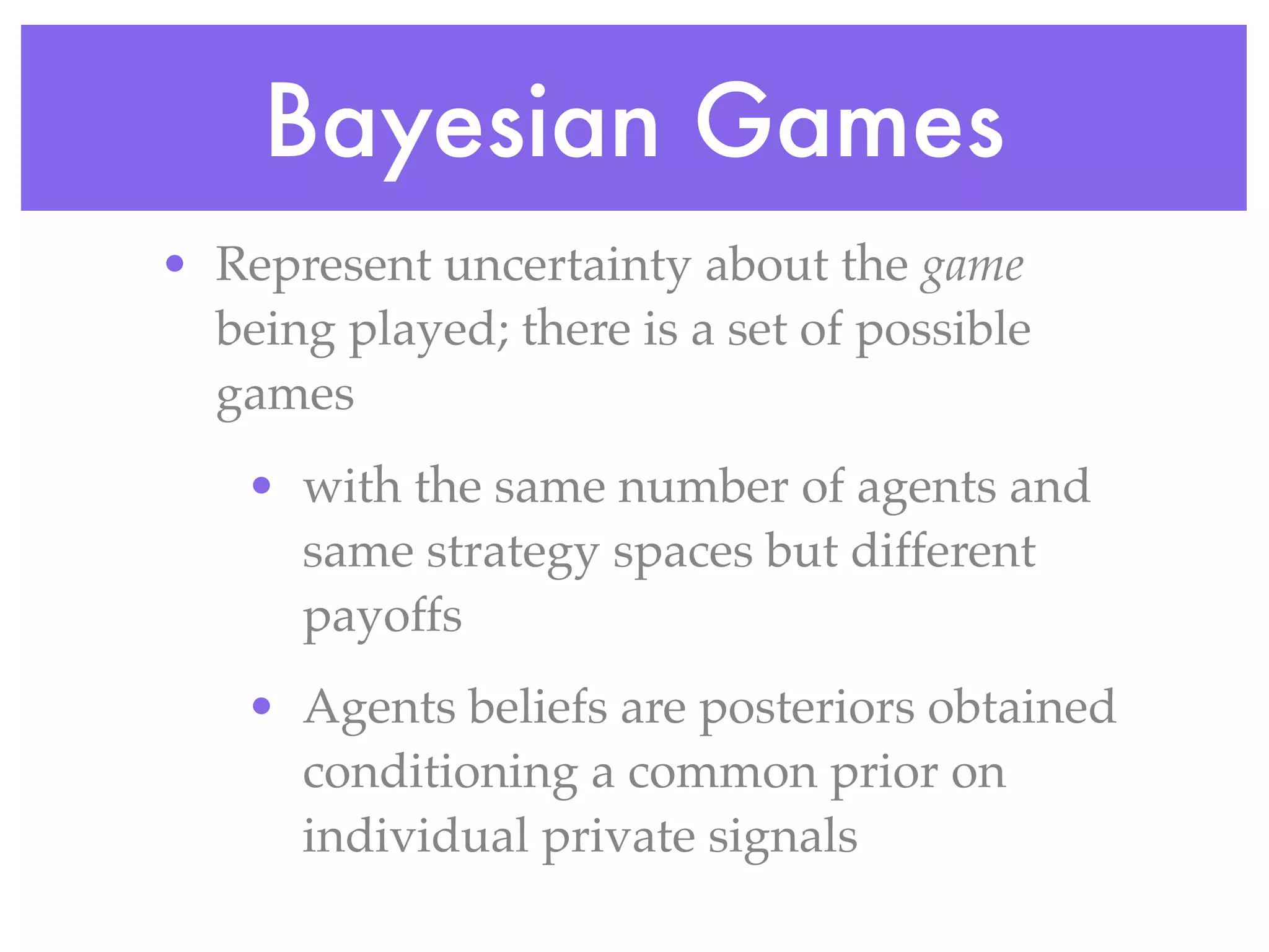
![Outcomes
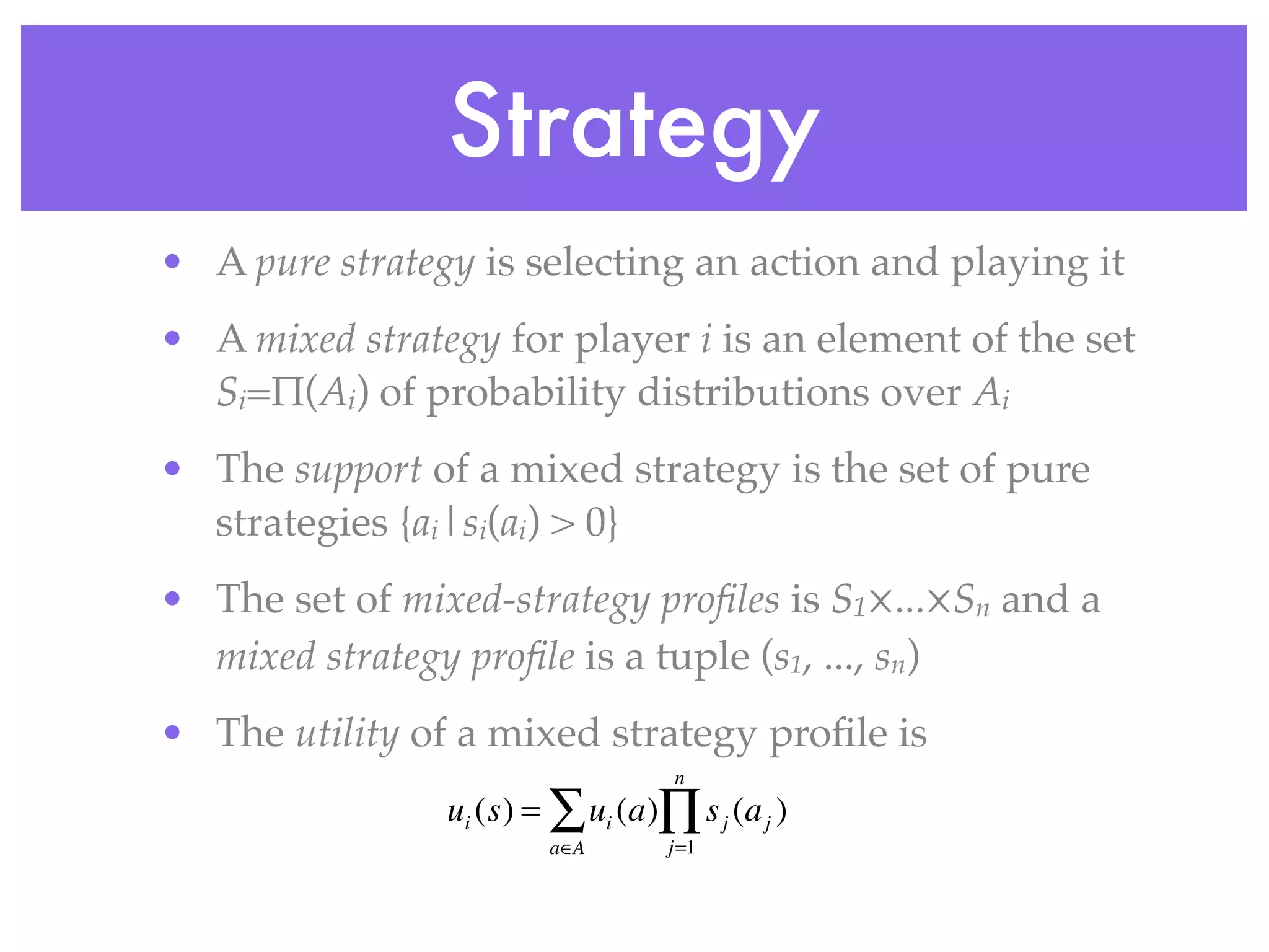
• Let O be a finite set of outcomes
• A lottery is a probability distribution
over O l = [ p1 : o1 ,…, pk : ok ]
oi ∈O pi ∈[0,1]
k
∑p i =1
i=1
• We assume agents can rank outcomes
and lotteries with a utility function](https://image.slidesharecdn.com/game-theory-120604121557-phpapp01/75/Game-theory-4-2048.jpg)

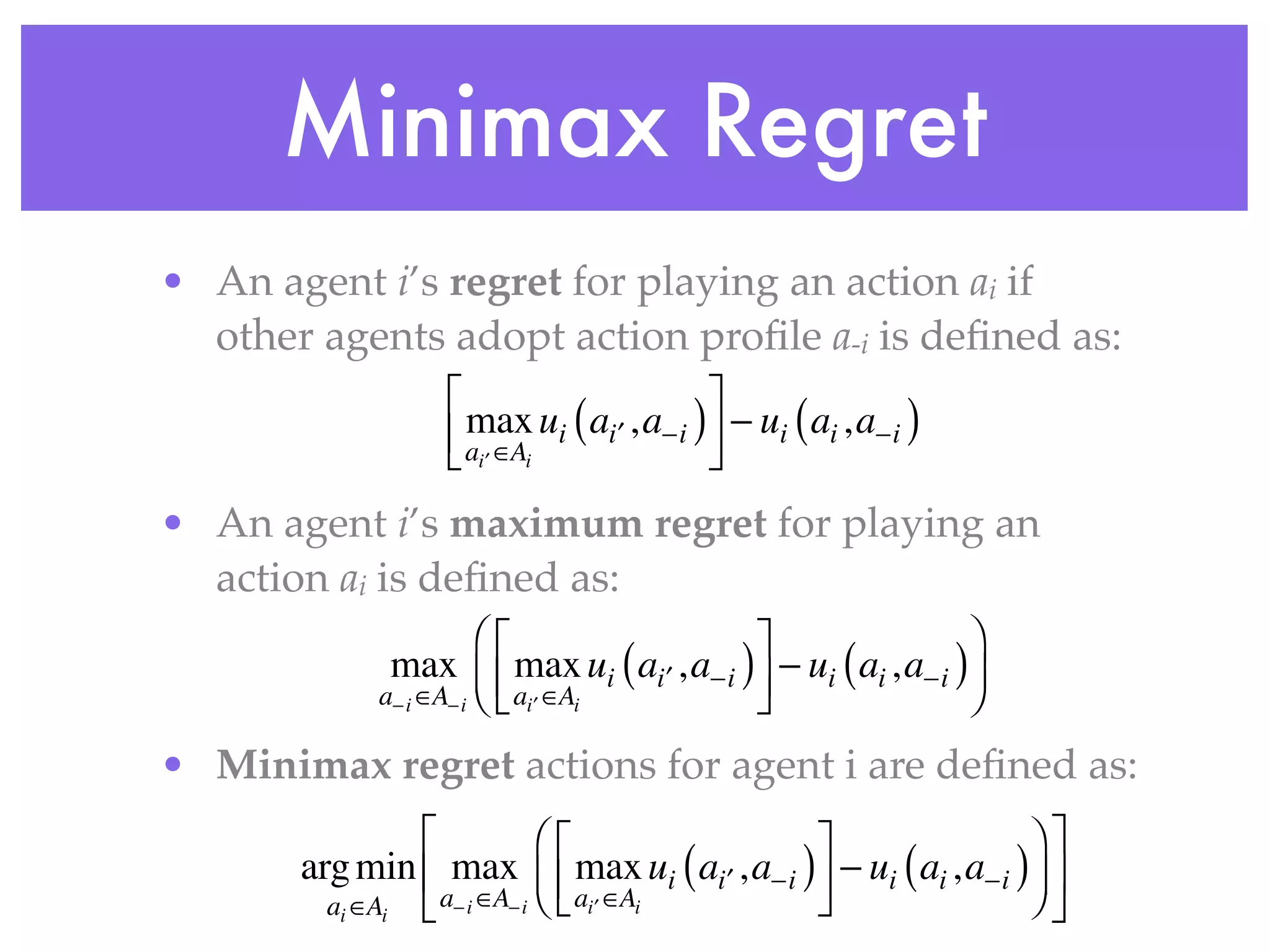
![Maxmin vs. Minmax Regret
L R
regret(T ,[R])= 1− 1+ =
regret(B,[R]) = 1− 1 = 0
regret(T ,[L]) = 100 − 100 = 0 T 100, a 1-!, b
regret(B,[L]) = 100 − 2 = 98
max regret(T )= max{,0} = B 2, c 1, d
max regret(B) = max{98,0} = 98
P1 Maxmin is B (why?), his
Minimax Regret strategy is T](https://image.slidesharecdn.com/game-theory-120604121557-phpapp01/75/Game-theory-35-2048.jpg)


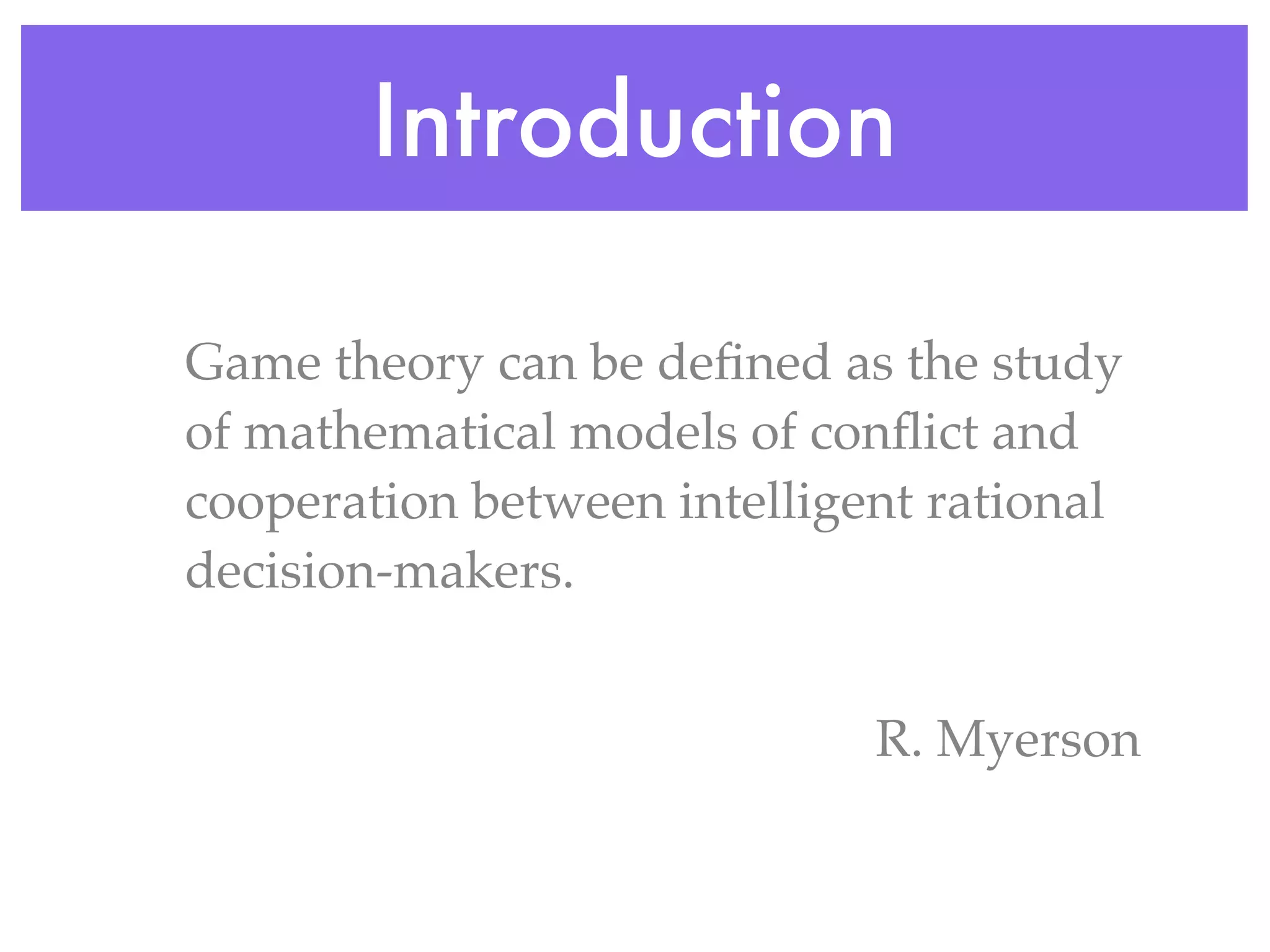
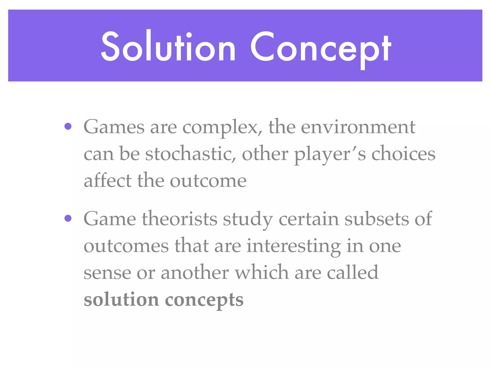
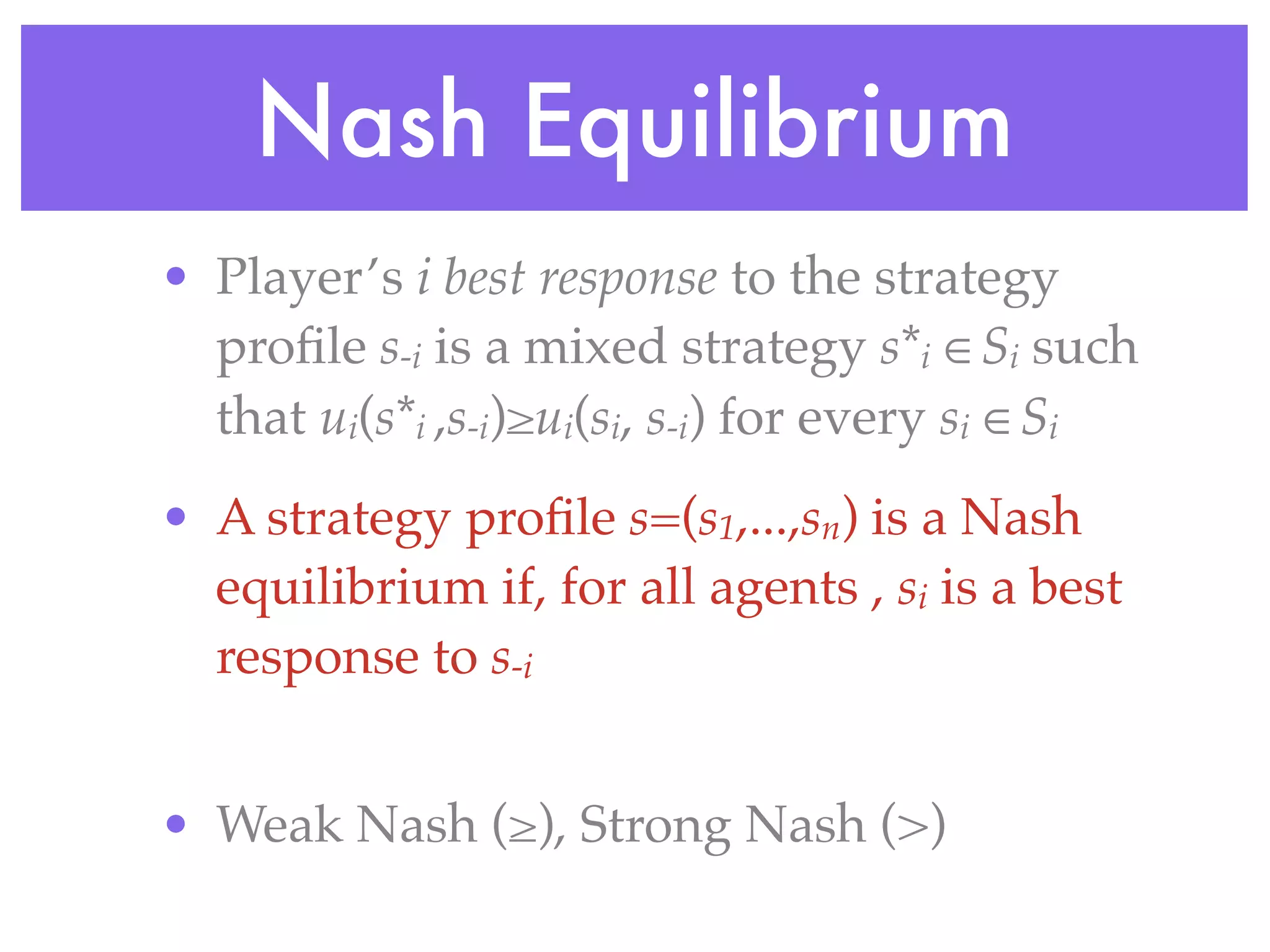
Game theory is the study of mathematical models of conflict and cooperation between rational decision-makers. It analyzes strategic decision-making through modeling games with several players under conditions of both cooperation and conflict. Game theory looks at solution concepts such as Nash equilibria, which are strategy profiles where each player's strategy is a best response to the other players' strategies. It is used to understand outcomes in strategic interactions in economics, political science, and other fields.


![Game theory intro_and_questions_2009[1]](https://cdn.slidesharecdn.com/ss_thumbnails/gametheoryintroandquestions20091-140204051533-phpapp02-thumbnail.jpg?width=640&height=640&fit=bounds)


![Coded Agents – with UiPath SDK + LangGraph [Virtual Hands-on Workshop]](https://cdn.slidesharecdn.com/ss_thumbnails/codedagentsdeck-251215155422-5497c599-thumbnail.jpg?width=640&height=640&fit=bounds)


