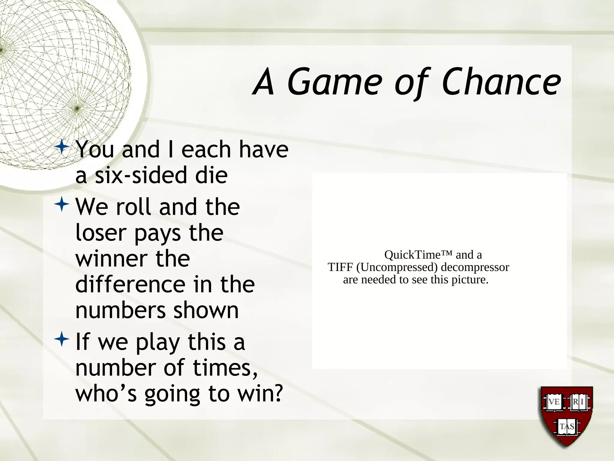
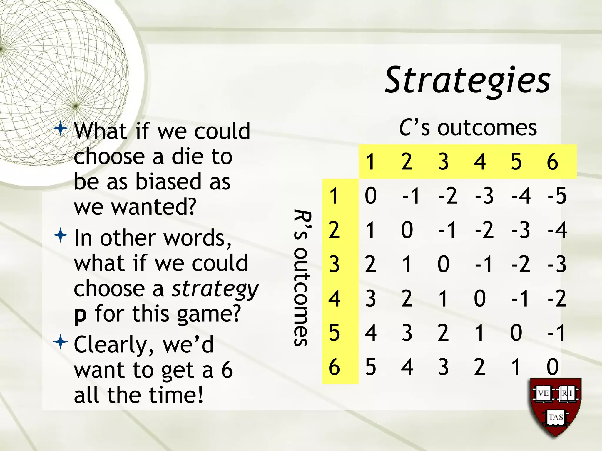
A very little Game Theory 
Math 20 
Linear Algebra and Multivariable 
Calculus 
October 13, 2004
A Game of Chance 
You and I each have 
a six-sided die 
We roll and the 
loser pays the 
winner the 
difference in the 
numbers shown 
If we play this a 
number of times, 
who’s going to win? 
QuickTime™ and a 
TIFF (Uncompressed) decompressor 
are needed to see this picture.
The Payoff Matrix 
Lists one player’s 
(call him/her R) 
possible outcomes 
versus another 
player’s (call him/her 
C) outcomes 
Each aij represents the 
payoff from C to R if 
outcomes i for R and j 
for C occur (a zero-sum 
game). 
C’s outcomes 
1 2 3 4 5 6 R’s outcomes 
1 0 -1 -2 -3 -4 -5 
2 1 0 -1 -2 -3 -4 
3 2 1 0 -1 -2 -3 
4 3 2 1 0 -1 -2 
5 4 3 2 1 0 -1 
6 5 4 3 2 1 0
Expected Value 
Let the probabilities of R’s outcomes and C’s 
outcomes be given by probability vectors 
   
p = [p1 p2 L pn ] 
   
q = 
⎡ 
q1 
q2 
M 
qn 
⎢⎢⎢⎢ 
⎣ 
⎤ 
⎥⎥⎥⎥ 
⎦
Expected Value 
The probability of R having outcome i 
and C having outcome j is therefore 
piqj. 
The expected value of R’s payoff is 
nå 
E(p,q) = pi aijqj 
i,j=1 
= pAq
Expected Value of this Game 
   
1 
6 
1 
6 
1 
6 
1 
6 
1 
6 
1 
6 
⎡⎣ ⎢ 
⎤⎦ ⎥ 
⋅ 
⎡ 
0 −1 −2 −3 −4 −5 
1 0 −1 −2 −3 −4 
2 1 0 −1 −2 −3 
3 2 1 0 −1 2 
4 3 2 1 0 −1 
5 4 3 2 1 0 
⎢⎢⎢⎢⎢⎢⎢ 
⎣ 
⎤ 
⎥⎥⎥⎥⎥⎥⎥ 
⋅ 
⎦ 
⎡ 
1 
⎢⎢⎢⎢⎢⎢⎢⎢⎢⎢⎢⎢ 
61 
61 
61 
61 
61 
⎣ 
6 
⎤ 
⎥⎥⎥⎥⎥⎥⎥⎥⎥⎥⎥⎥ 
⎦ 
   
= 1 
6 
⋅ [1 1 1 1 1 1] ⋅ 
⎡ 
−15 
−9 
−3 
3 
9 
15 
⎢⎢⎢⎢⎢⎢⎢ 
⎣ 
⎤ 
⎥⎥⎥⎥⎥⎥⎥ 
⋅ 1 
6 
⎦ 
= 0 
A “fair game” if the dice are fair.
Expected value 
with an unfair die 
Suppose 
Then 
   
p = 
1 
10 
1 
10 
1 
5 
1 
5 
1 
5 
1 
5 
⎡⎣ ⎢ 
⎤⎦ ⎥ 
   
E(p,q) = 
1 
10 
1 
10 
1 
5 
1 
5 
1 
5 
1 
5 
⎡⎣ ⎢ 
⎤⎦ ⎥ 
⋅ 
⎡ 
⎢⎢⎢⎢⎢⎢⎢ ⎤ 
0 −1 −2 −3 −4 −5 
1 0 −1 −2 −3 −4 
2 1 0 −1 −2 −3 
3 2 1 0 −1 2 
4 3 2 1 0 −1 
5 4 3 2 1 0 
⎣ 
⎥⎥⎥⎥⎥⎥⎥ 
⋅ 
⎦ 
⎡ 
1 
⎢⎢⎢⎢⎢⎢⎢⎢⎢⎢⎢⎢ 
61 
61 
61 
61 
61 
⎣ 
6 
⎤ 
⎥⎥⎥⎥⎥⎥⎥⎥⎥⎥⎥⎥ 
⎦ 
= 
1 
10 
⋅ [1 1 2 2 2 2] ⋅ 
⎡ 
−15 
−9 
−3 
3 
9 
15 
⎢⎢⎢⎢⎢⎢⎢ 
⎣ 
⎤ 
⎥⎥⎥⎥⎥⎥⎥ 
⋅ 1 
6 
⎦ 
= 
1 
60 
((−15) + (−9) + 2(−3) + 2⋅ 3+ 2⋅ 9 + 2 ⋅15) = 
24 
60 
= 
2 
5
Strategies 
What if we could 
choose a die to 
be as biased as 
we wanted? 
In other words, 
what if we could 
choose a strategy 
p for this game? 
Clearly, we’d 
want to get a 6 
all the time! 
C’s outcomes 
1 2 3 4 5 6 R’s outcomes 
1 0 -1 -2 -3 -4 -5 
2 1 0 -1 -2 -3 -4 
3 2 1 0 -1 -2 -3 
4 3 2 1 0 -1 -2 
5 4 3 2 1 0 -1 
6 5 4 3 2 1 0
Flu Vaccination 
Suppose there are two 
flu strains, and we have 
two flu vaccines to 
combat them. 
We don’t know 
distribution of strains 
Neither pure strategy is 
the clear favorite 
Is there a combination of 
vaccines that maximizes 
immunity? 
Strain 
1 2 
Vaccine 
1 0.85 0.70 
2 0.60 0.90
Fundamental Theorem of 
Zero-Sum Games 
There exist optimal strategies p* for R and 
q* for C such that for all strategies p and q: 
E(p*,q) ≥ E(p*,q*) ≥ E(p,q*) 
E(p*,q*) is called the value v of the game 
In other words, R can guarantee a lower 
bound on his/her payoff and C can guarantee 
an upper bound on how much he/she loses 
This value could be negative in which case C 
has the advantage
Fundamental Problem of 
Zero-Sum games 
Find the p* and q*! 
In general, this requires linear 
programming. Next week! 
There are some games in which we can 
find optimal strategies now: 
Strictly-determined games 
2 2 non-strictly-determined games
Network Programming 
Suppose we have two 
networks, NBC and CBS 
Each chooses which 
program to show in a 
certain time slot 
Viewer share varies 
depending on these 
combinations 
How can NBC get the 
most viewers? 
QuickTime™ and a 
TIFF (Uncompressed) decompressor 
are needed to see this picture. 
TIFFQ (uUicnkcTomimper™ess aendd) daecompressor are needed to see this picture.
Payoff Matrix 
CBS shows 
60 Minutes 
Survivor 
CSI 
Everybody Loves Raymond 
NBC Shows 
Friends 60 20 30 55 
Dateline 50 75 45 60
NBC’s Strategy 
NBC wants to 
maximize NBC’s 
minimum share 
In airing Dateline, 
NBC’s share is at 
least 45 
This is a good 
strategy for NBC 
60 M 
Surv 
CSI 
ELR 
F 60 20 30 55 
DL 50 75 45 60 
LO 70 45 35 30
CBS’s Strategy 
CBS wants to 
minimize NBC’s 
maximum share 
In airing CSI, CBS 
keeps NBC’s share 
no bigger than 45 
This is a good 
strategy for CBS 
60 M 
Surv 
CSI 
ELR 
F 60 20 30 55 
DL 50 75 45 60 
LO 70 45 35 30
Equilibrium 
(Dateline,CSI) is an 
equilibrium pair of 
strategies 
Assuming NBC airs 
Dateline, CBS’s 
best choice is to air 
CSI, and vice versa 
60 M 
Surv 
CSI 
ELR 
F 60 20 30 55 
DL 50 75 45 60 
LO 70 45 35 30
Characteristics of an 
Equlibrium 
Let A be a payoff matrix. A saddle point is 
an entry ars which is the minimum entry in its 
row and the maximum entry in its column. 
A game whose payoff matrix has a saddle 
point is called strictly determined 
Payoff matrices can have multiple saddle 
points
Pure Strategies are optimal 
in Strictly-Determined Games 
If ars is a saddle 
point, then er 
T is an 
optimal strategy for 
R and es is an 
optimal strategy for 
C. 
QuickTime™ and a 
TIFF (Uncompressed) decompressor 
are needed to see this picture.
Proof 
T ,q) = e r T 
Aq = [ar1 ar2 L arn ]× 
E(er 
q1 
q2 
é 
êêêê 
úúúú 
M 
qn 
ë 
ù 
û 
= ar1q1 
+ar2q2 
+L +arnqn 
³ arsq1 
+arsq2 
+L +arsqn 
= ars(q1 
+L + qn ) = ars = E(er T 
,es)
Proof 
E(p,es ) = pAes = p1 p2 
[ L pm ]× 
a1s 
a2 
é 
êêêê 
úúúú 
s 
M 
ams 
ë 
ù 
û 
= p1 a1s + p2 
a2 
s +L + pmams 
£ p1 
ars + p2 
ars +L + pmars 
= ( p1 
+ p2 
+L + pm )ars = ars = E(er T 
,es)
Proof 
So for all strategies p and q: 
E(er 
T,q) ≥ E(er 
T,es) ≥ E(p,es) 
Therefore we have found the optimal 
strategies
2x2 non-strictly determined 
In this case we can compute E(p,q) by 
hand in terms of p1 and q1 
E(p,q) = [p1 p2 ] ⋅ 
⎡ 
a11 a12 
a21 a22 
⎣ ⎢ 
⎤ 
⋅ 
⎦ ⎥ 
⎡ 
q1 
q2 
⎣ ⎢ 
⎤ 
⎦ ⎥ 
= p1a11q1 + p1a12q2 + p2a21q1 + p2a22q2 
= p1a11q1 + p1a12(1−q1) + (1− p1)a21q1 + (1− p1)a22(1−q1) 
= (a11 + a22 − a12 − a21)p1 −(a22 − a21[ )]q1 + (a12 − a22 )p1 + a22
Optimal Strategy for 2x2 non-SD 
∗ a22 − a21 
a11 + a22 − a12 − a21 
Let 
This is between 0 and 1 if A has no 
saddle points 
   
Then 
p1 = p1 
; p2 =1− p1 
E(p,q) = 
(a12 − a22 )(a22 − a21) 
a11 + a22 − a12 − a21 
+ a22 
= 
a11a22 − a12a21 
a11 + a22 − a12 − a21
Optimal set of strategies 
We have 
ù 
û ú 
2 
a22 - a21 
1 + a22 - a1 
2 - a21 
a11 + a22 - a12 - a2 
p* = 
1 
a11 - a1 
a1 
é 
ë ê 
úúúú 
1 
êêêê 
q* = 
a22 - a12 
a11 + a22 - a12 - a2 
a11 - a21 
1 
a11 + a22 - a12 - a2 
ù 
é 
û 
ë 
1a22 - a12a2 
1 
a1 
a11 + a22 - a12 - a2 
v= 
1
Flu Vaccination 
Strain 
1 2 
Vaccine 
1 0.85 0.70 
2 0.60 0.90 
* = 
p1 
.90 - .60 
.85 + .90 - .70 - .60 
= 
.30 
.45 
= 
2 
3 
* = 
p2 
1 
3 
* = 
q1 
.90 - .70 
.85 + .90 - .70 - .60 
= 
.20 
.45 
= 
4 
9 
* = 
q2 
5 
9 
v= 
(.85)(.90) - (.70)(.60) 
.85 + .90 - .70 - .60 
= 
.345 
.45 
= .766K
Flu Vaccination 
Strain 
1 2 
Vaccine 
1 0.85 0.70 
2 0.60 0.90 
So we should give 
2/3 of the 
population vaccine 
1 and 1/3 vaccine 2 
The worst that 
could happen is a 
4:5 distribution of 
strains 
In this case we 
cover 76.7% of pop
Other Applications of GT 
War 
Battle of Bismarck 
Sea 
Business 
Product Introduction 
Pricing 
Dating 
QuickTime™ and a 
TIFF (Uncompressed) decompressor 
are needed to see this picture.

Game theory

  • 1.
    A very littleGame Theory Math 20 Linear Algebra and Multivariable Calculus October 13, 2004
  • 2.
    A Game ofChance You and I each have a six-sided die We roll and the loser pays the winner the difference in the numbers shown If we play this a number of times, who’s going to win? QuickTime™ and a TIFF (Uncompressed) decompressor are needed to see this picture.
  • 3.
    The Payoff Matrix Lists one player’s (call him/her R) possible outcomes versus another player’s (call him/her C) outcomes Each aij represents the payoff from C to R if outcomes i for R and j for C occur (a zero-sum game). C’s outcomes 1 2 3 4 5 6 R’s outcomes 1 0 -1 -2 -3 -4 -5 2 1 0 -1 -2 -3 -4 3 2 1 0 -1 -2 -3 4 3 2 1 0 -1 -2 5 4 3 2 1 0 -1 6 5 4 3 2 1 0
  • 4.
    Expected Value Letthe probabilities of R’s outcomes and C’s outcomes be given by probability vectors   p = [p1 p2 L pn ]   q = ⎡ q1 q2 M qn ⎢⎢⎢⎢ ⎣ ⎤ ⎥⎥⎥⎥ ⎦
  • 5.
    Expected Value Theprobability of R having outcome i and C having outcome j is therefore piqj. The expected value of R’s payoff is nå E(p,q) = pi aijqj i,j=1 = pAq
  • 6.
    Expected Value ofthis Game   1 6 1 6 1 6 1 6 1 6 1 6 ⎡⎣ ⎢ ⎤⎦ ⎥ ⋅ ⎡ 0 −1 −2 −3 −4 −5 1 0 −1 −2 −3 −4 2 1 0 −1 −2 −3 3 2 1 0 −1 2 4 3 2 1 0 −1 5 4 3 2 1 0 ⎢⎢⎢⎢⎢⎢⎢ ⎣ ⎤ ⎥⎥⎥⎥⎥⎥⎥ ⋅ ⎦ ⎡ 1 ⎢⎢⎢⎢⎢⎢⎢⎢⎢⎢⎢⎢ 61 61 61 61 61 ⎣ 6 ⎤ ⎥⎥⎥⎥⎥⎥⎥⎥⎥⎥⎥⎥ ⎦   = 1 6 ⋅ [1 1 1 1 1 1] ⋅ ⎡ −15 −9 −3 3 9 15 ⎢⎢⎢⎢⎢⎢⎢ ⎣ ⎤ ⎥⎥⎥⎥⎥⎥⎥ ⋅ 1 6 ⎦ = 0 A “fair game” if the dice are fair.
  • 7.
    Expected value withan unfair die Suppose Then   p = 1 10 1 10 1 5 1 5 1 5 1 5 ⎡⎣ ⎢ ⎤⎦ ⎥   E(p,q) = 1 10 1 10 1 5 1 5 1 5 1 5 ⎡⎣ ⎢ ⎤⎦ ⎥ ⋅ ⎡ ⎢⎢⎢⎢⎢⎢⎢ ⎤ 0 −1 −2 −3 −4 −5 1 0 −1 −2 −3 −4 2 1 0 −1 −2 −3 3 2 1 0 −1 2 4 3 2 1 0 −1 5 4 3 2 1 0 ⎣ ⎥⎥⎥⎥⎥⎥⎥ ⋅ ⎦ ⎡ 1 ⎢⎢⎢⎢⎢⎢⎢⎢⎢⎢⎢⎢ 61 61 61 61 61 ⎣ 6 ⎤ ⎥⎥⎥⎥⎥⎥⎥⎥⎥⎥⎥⎥ ⎦ = 1 10 ⋅ [1 1 2 2 2 2] ⋅ ⎡ −15 −9 −3 3 9 15 ⎢⎢⎢⎢⎢⎢⎢ ⎣ ⎤ ⎥⎥⎥⎥⎥⎥⎥ ⋅ 1 6 ⎦ = 1 60 ((−15) + (−9) + 2(−3) + 2⋅ 3+ 2⋅ 9 + 2 ⋅15) = 24 60 = 2 5
  • 8.
    Strategies What ifwe could choose a die to be as biased as we wanted? In other words, what if we could choose a strategy p for this game? Clearly, we’d want to get a 6 all the time! C’s outcomes 1 2 3 4 5 6 R’s outcomes 1 0 -1 -2 -3 -4 -5 2 1 0 -1 -2 -3 -4 3 2 1 0 -1 -2 -3 4 3 2 1 0 -1 -2 5 4 3 2 1 0 -1 6 5 4 3 2 1 0
  • 9.
    Flu Vaccination Supposethere are two flu strains, and we have two flu vaccines to combat them. We don’t know distribution of strains Neither pure strategy is the clear favorite Is there a combination of vaccines that maximizes immunity? Strain 1 2 Vaccine 1 0.85 0.70 2 0.60 0.90
  • 10.
    Fundamental Theorem of Zero-Sum Games There exist optimal strategies p* for R and q* for C such that for all strategies p and q: E(p*,q) ≥ E(p*,q*) ≥ E(p,q*) E(p*,q*) is called the value v of the game In other words, R can guarantee a lower bound on his/her payoff and C can guarantee an upper bound on how much he/she loses This value could be negative in which case C has the advantage
  • 11.
    Fundamental Problem of Zero-Sum games Find the p* and q*! In general, this requires linear programming. Next week! There are some games in which we can find optimal strategies now: Strictly-determined games 2 2 non-strictly-determined games
  • 12.
    Network Programming Supposewe have two networks, NBC and CBS Each chooses which program to show in a certain time slot Viewer share varies depending on these combinations How can NBC get the most viewers? QuickTime™ and a TIFF (Uncompressed) decompressor are needed to see this picture. TIFFQ (uUicnkcTomimper™ess aendd) daecompressor are needed to see this picture.
  • 13.
    Payoff Matrix CBSshows 60 Minutes Survivor CSI Everybody Loves Raymond NBC Shows Friends 60 20 30 55 Dateline 50 75 45 60
  • 14.
    NBC’s Strategy NBCwants to maximize NBC’s minimum share In airing Dateline, NBC’s share is at least 45 This is a good strategy for NBC 60 M Surv CSI ELR F 60 20 30 55 DL 50 75 45 60 LO 70 45 35 30
  • 15.
    CBS’s Strategy CBSwants to minimize NBC’s maximum share In airing CSI, CBS keeps NBC’s share no bigger than 45 This is a good strategy for CBS 60 M Surv CSI ELR F 60 20 30 55 DL 50 75 45 60 LO 70 45 35 30
  • 16.
    Equilibrium (Dateline,CSI) isan equilibrium pair of strategies Assuming NBC airs Dateline, CBS’s best choice is to air CSI, and vice versa 60 M Surv CSI ELR F 60 20 30 55 DL 50 75 45 60 LO 70 45 35 30
  • 17.
    Characteristics of an Equlibrium Let A be a payoff matrix. A saddle point is an entry ars which is the minimum entry in its row and the maximum entry in its column. A game whose payoff matrix has a saddle point is called strictly determined Payoff matrices can have multiple saddle points
  • 18.
    Pure Strategies areoptimal in Strictly-Determined Games If ars is a saddle point, then er T is an optimal strategy for R and es is an optimal strategy for C. QuickTime™ and a TIFF (Uncompressed) decompressor are needed to see this picture.
  • 19.
    Proof T ,q)= e r T Aq = [ar1 ar2 L arn ]× E(er q1 q2 é êêêê úúúú M qn ë ù û = ar1q1 +ar2q2 +L +arnqn ³ arsq1 +arsq2 +L +arsqn = ars(q1 +L + qn ) = ars = E(er T ,es)
  • 20.
    Proof E(p,es )= pAes = p1 p2 [ L pm ]× a1s a2 é êêêê úúúú s M ams ë ù û = p1 a1s + p2 a2 s +L + pmams £ p1 ars + p2 ars +L + pmars = ( p1 + p2 +L + pm )ars = ars = E(er T ,es)
  • 21.
    Proof So forall strategies p and q: E(er T,q) ≥ E(er T,es) ≥ E(p,es) Therefore we have found the optimal strategies
  • 22.
    2x2 non-strictly determined In this case we can compute E(p,q) by hand in terms of p1 and q1 E(p,q) = [p1 p2 ] ⋅ ⎡ a11 a12 a21 a22 ⎣ ⎢ ⎤ ⋅ ⎦ ⎥ ⎡ q1 q2 ⎣ ⎢ ⎤ ⎦ ⎥ = p1a11q1 + p1a12q2 + p2a21q1 + p2a22q2 = p1a11q1 + p1a12(1−q1) + (1− p1)a21q1 + (1− p1)a22(1−q1) = (a11 + a22 − a12 − a21)p1 −(a22 − a21[ )]q1 + (a12 − a22 )p1 + a22
  • 23.
    Optimal Strategy for2x2 non-SD ∗ a22 − a21 a11 + a22 − a12 − a21 Let This is between 0 and 1 if A has no saddle points   Then p1 = p1 ; p2 =1− p1 E(p,q) = (a12 − a22 )(a22 − a21) a11 + a22 − a12 − a21 + a22 = a11a22 − a12a21 a11 + a22 − a12 − a21
  • 24.
    Optimal set ofstrategies We have ù û ú 2 a22 - a21 1 + a22 - a1 2 - a21 a11 + a22 - a12 - a2 p* = 1 a11 - a1 a1 é ë ê úúúú 1 êêêê q* = a22 - a12 a11 + a22 - a12 - a2 a11 - a21 1 a11 + a22 - a12 - a2 ù é û ë 1a22 - a12a2 1 a1 a11 + a22 - a12 - a2 v= 1
  • 25.
    Flu Vaccination Strain 1 2 Vaccine 1 0.85 0.70 2 0.60 0.90 * = p1 .90 - .60 .85 + .90 - .70 - .60 = .30 .45 = 2 3 * = p2 1 3 * = q1 .90 - .70 .85 + .90 - .70 - .60 = .20 .45 = 4 9 * = q2 5 9 v= (.85)(.90) - (.70)(.60) .85 + .90 - .70 - .60 = .345 .45 = .766K
  • 26.
    Flu Vaccination Strain 1 2 Vaccine 1 0.85 0.70 2 0.60 0.90 So we should give 2/3 of the population vaccine 1 and 1/3 vaccine 2 The worst that could happen is a 4:5 distribution of strains In this case we cover 76.7% of pop
  • 27.
    Other Applications ofGT War Battle of Bismarck Sea Business Product Introduction Pricing Dating QuickTime™ and a TIFF (Uncompressed) decompressor are needed to see this picture.