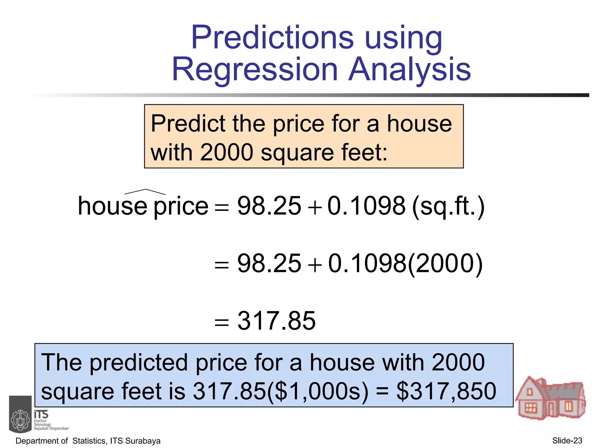
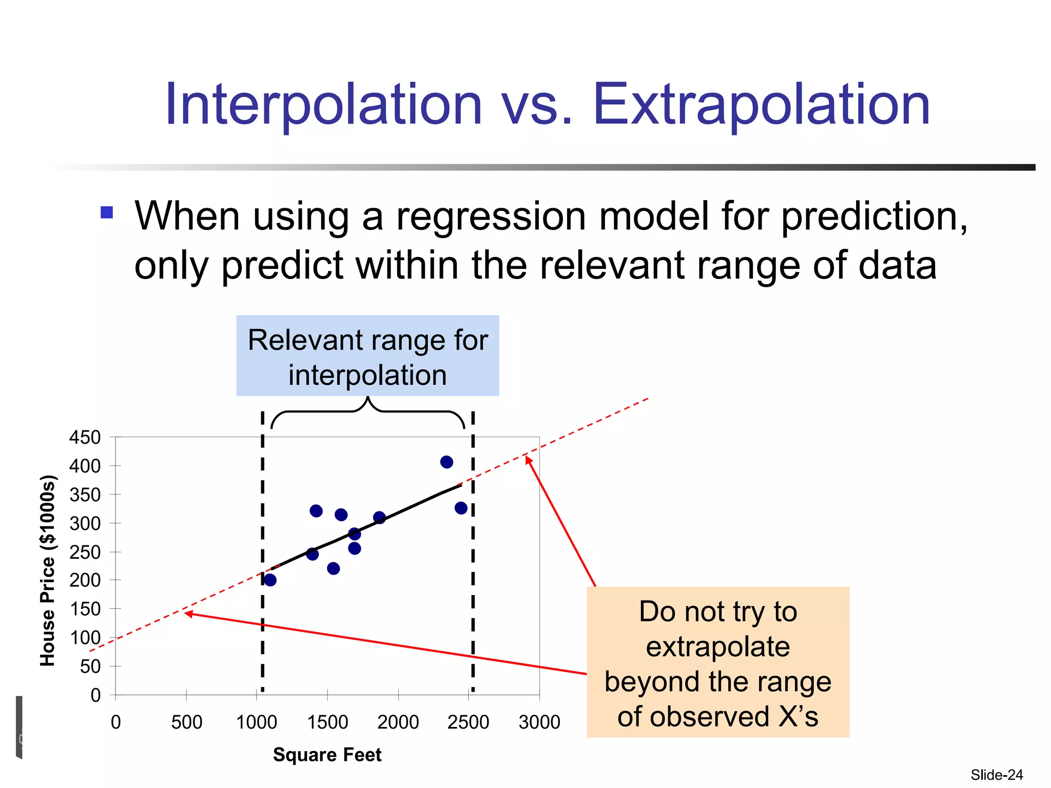
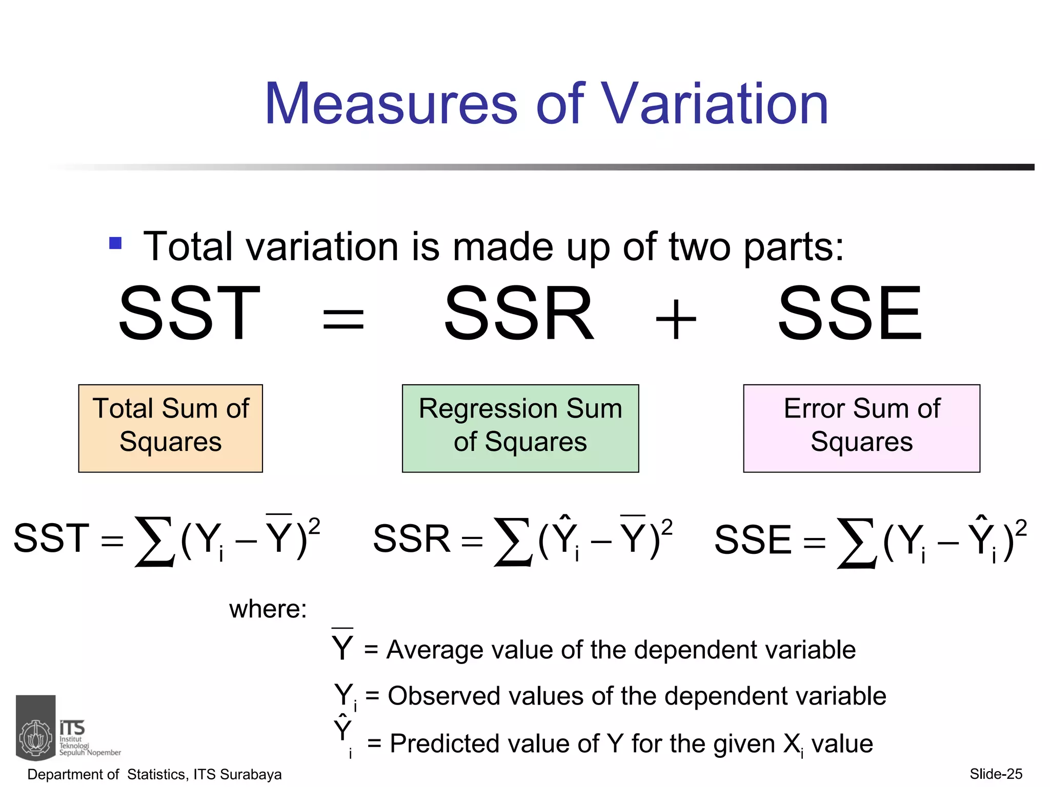
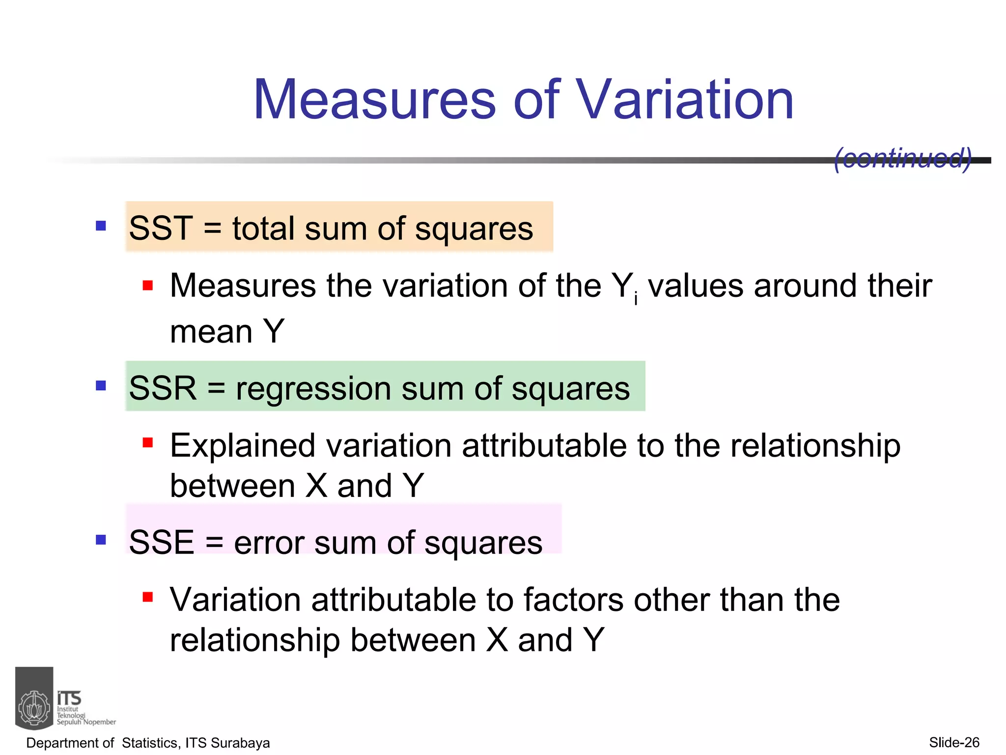
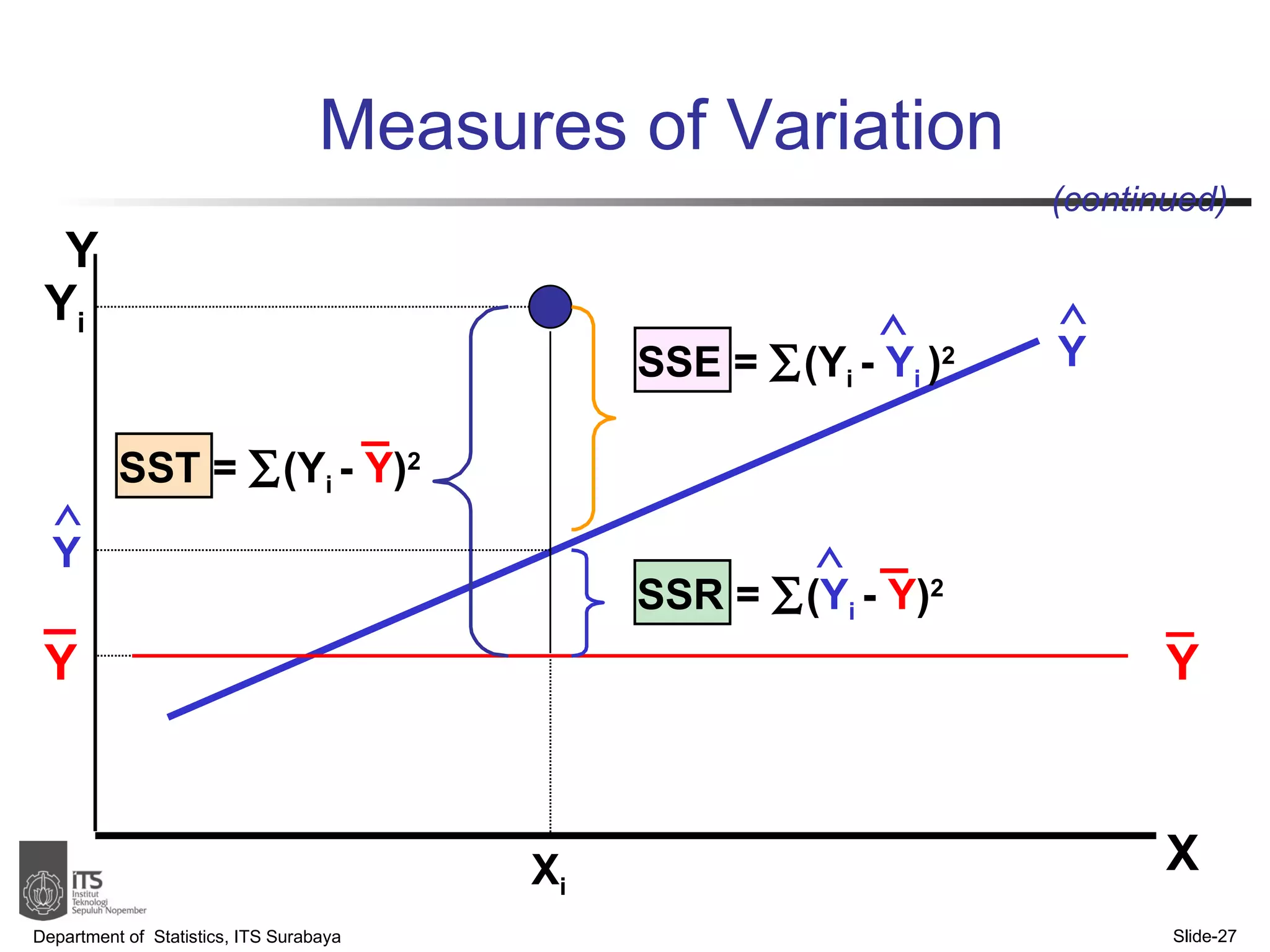
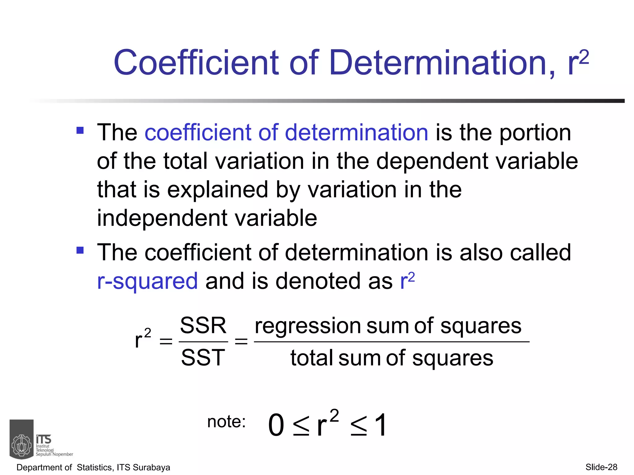
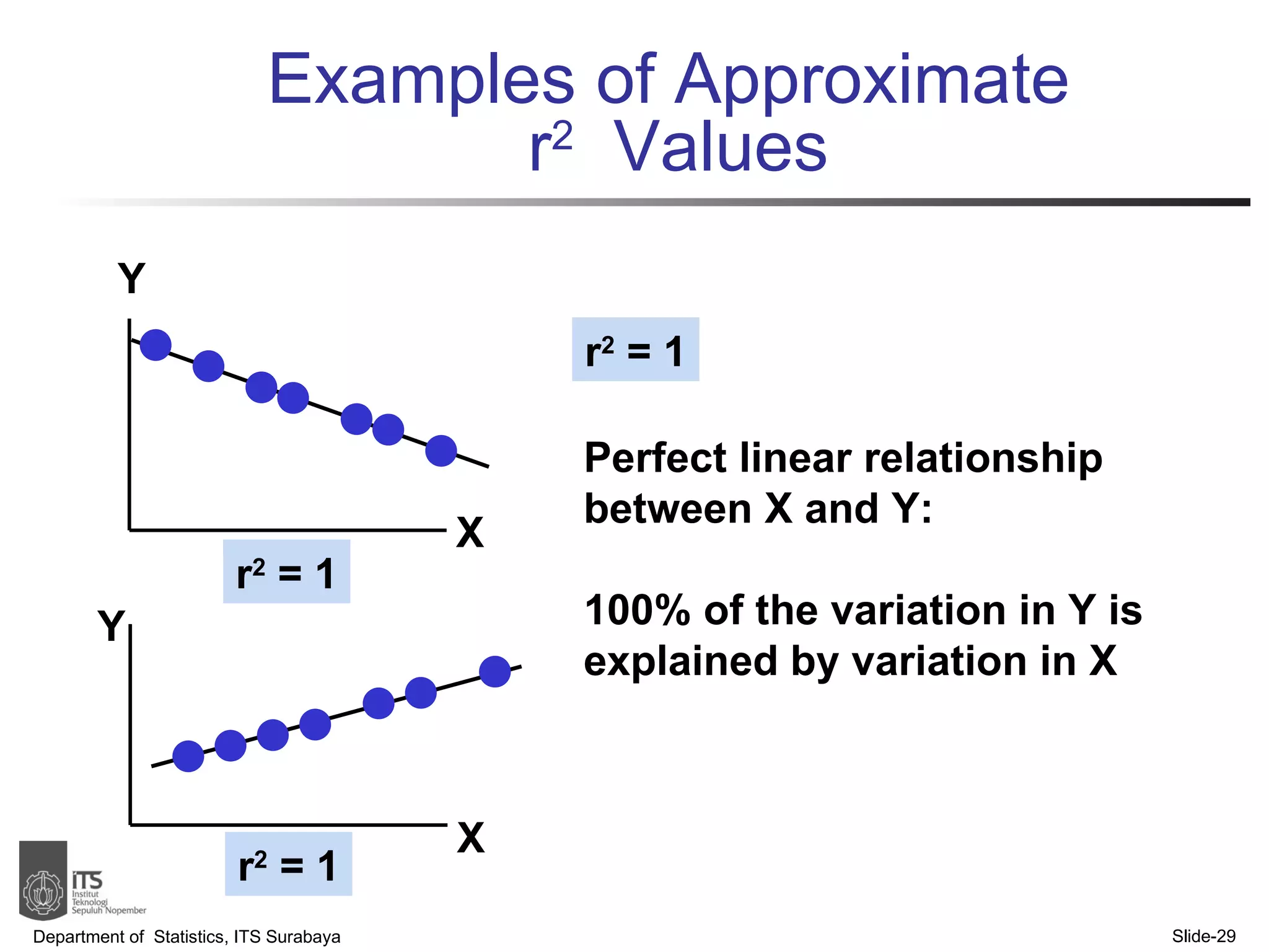
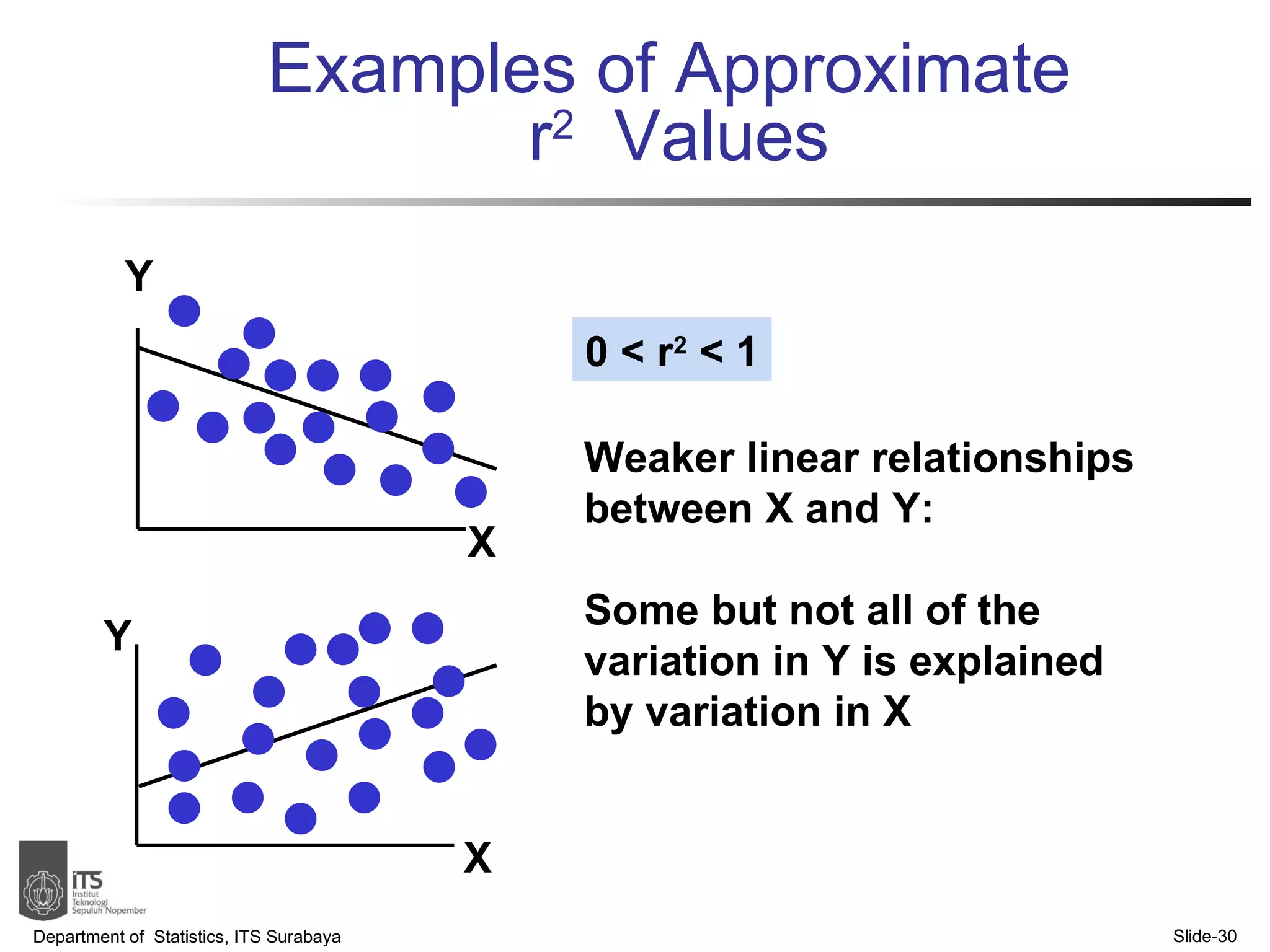
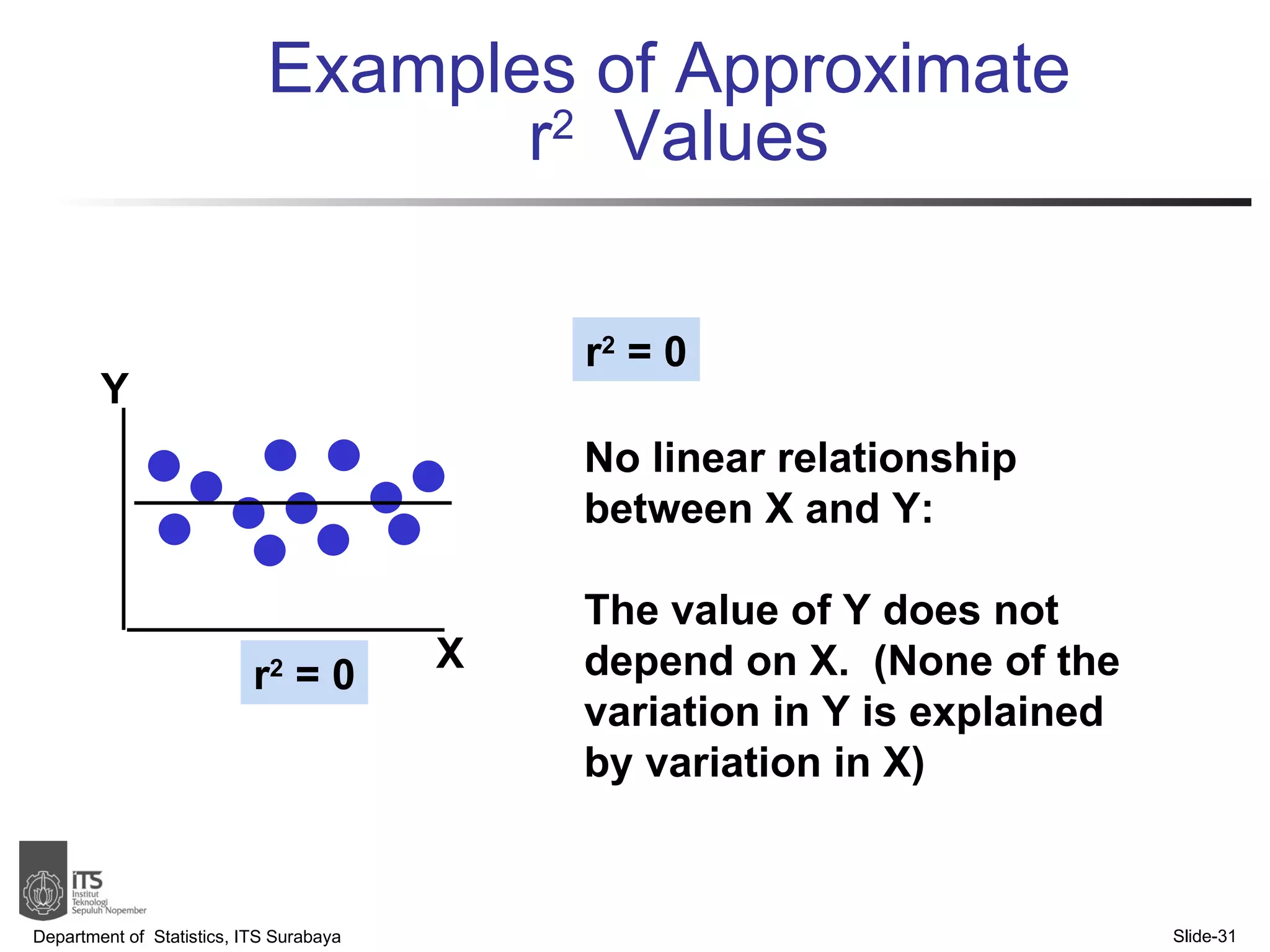
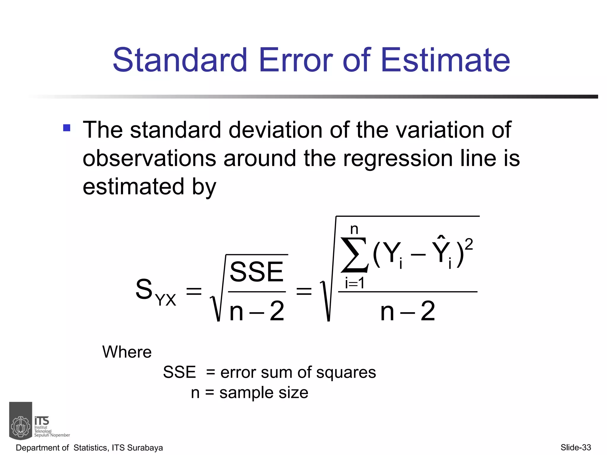
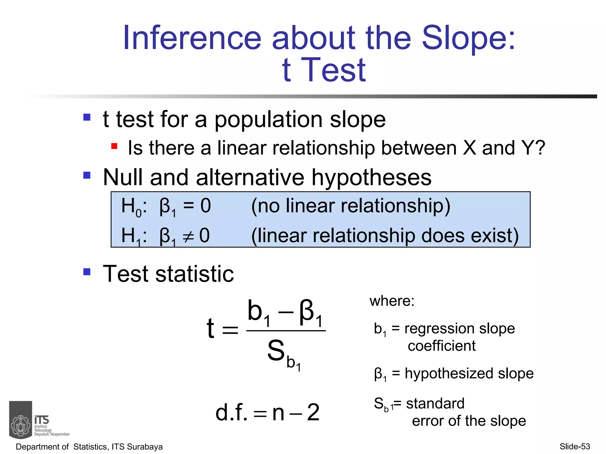
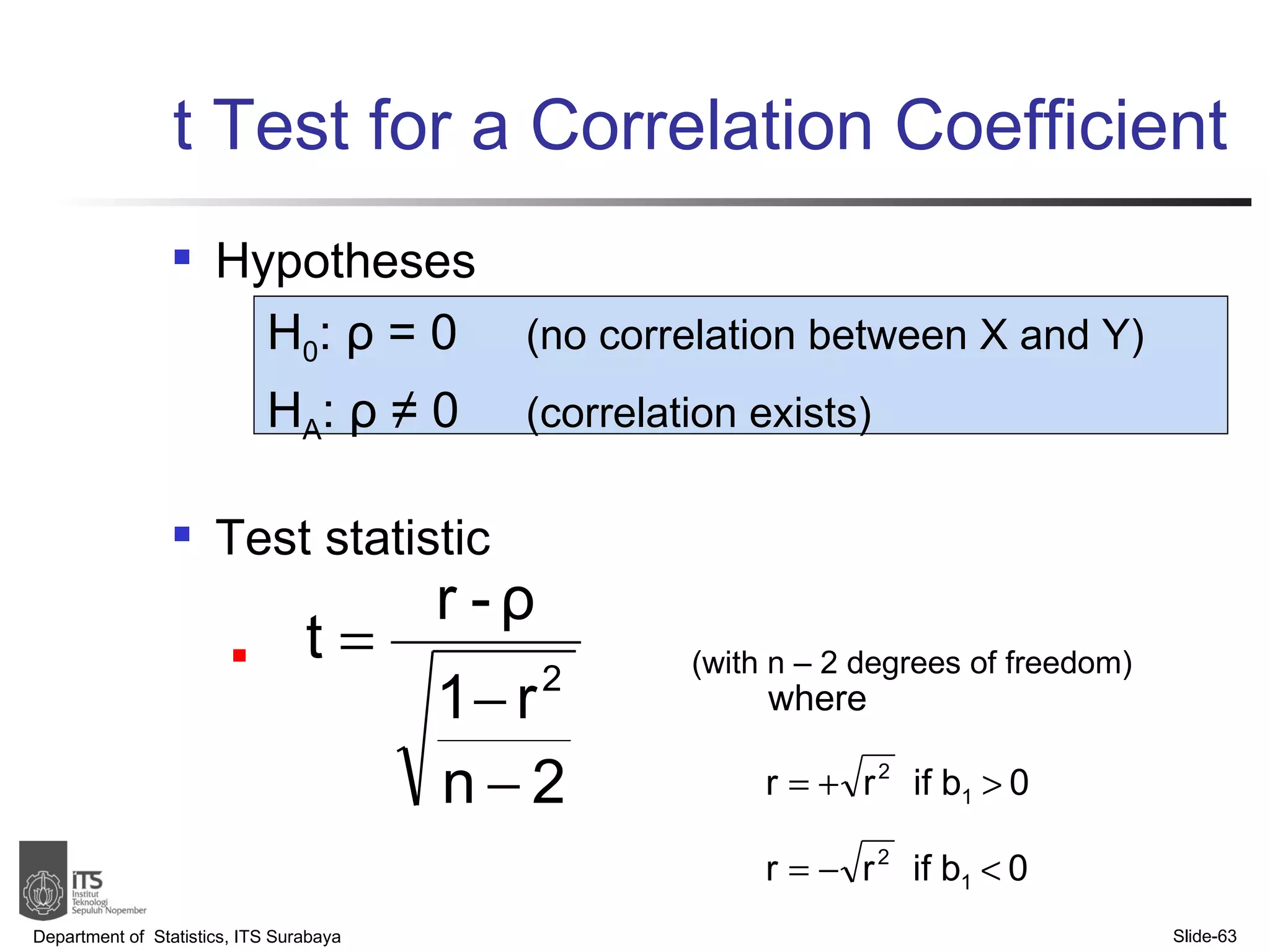
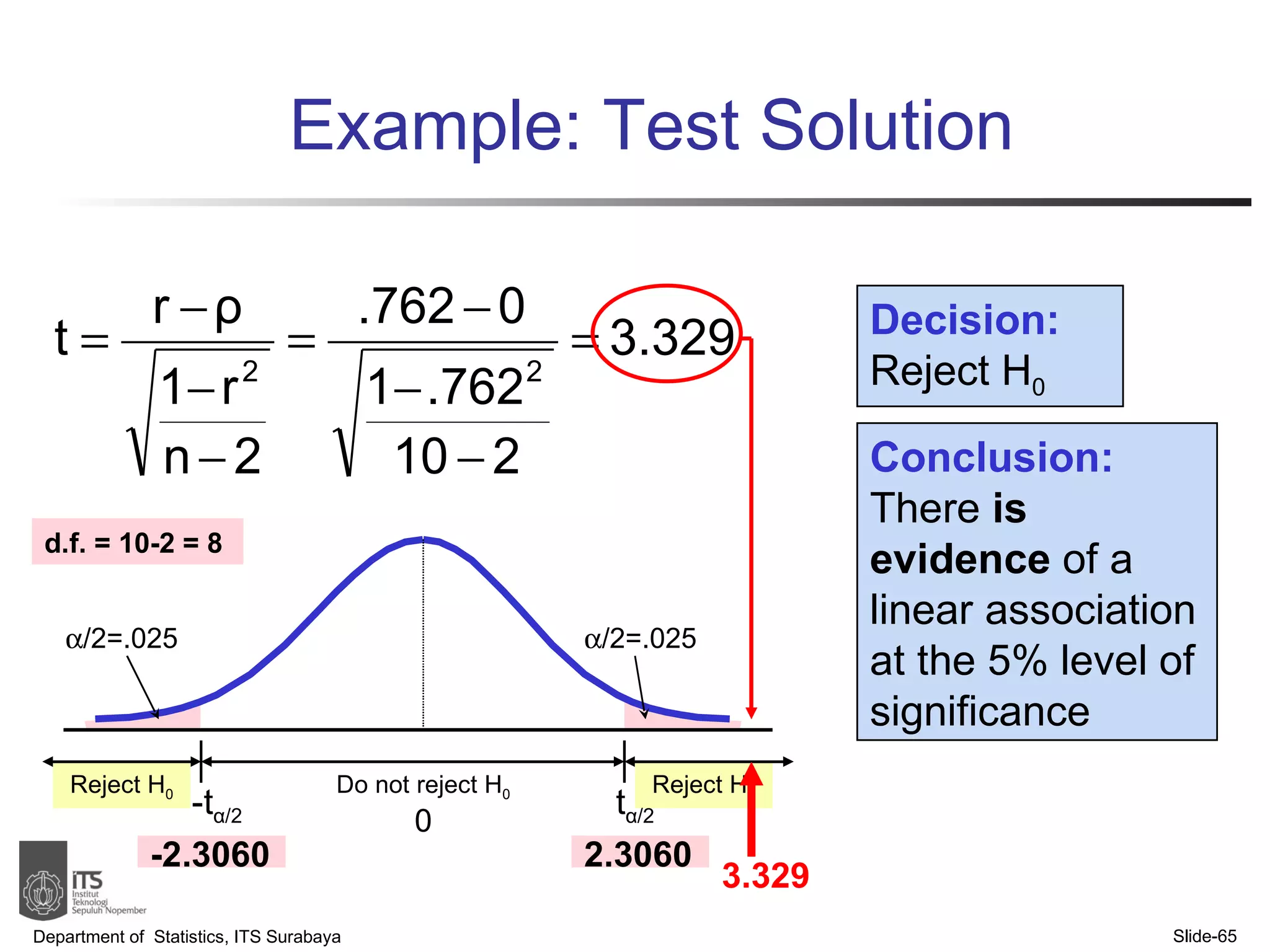
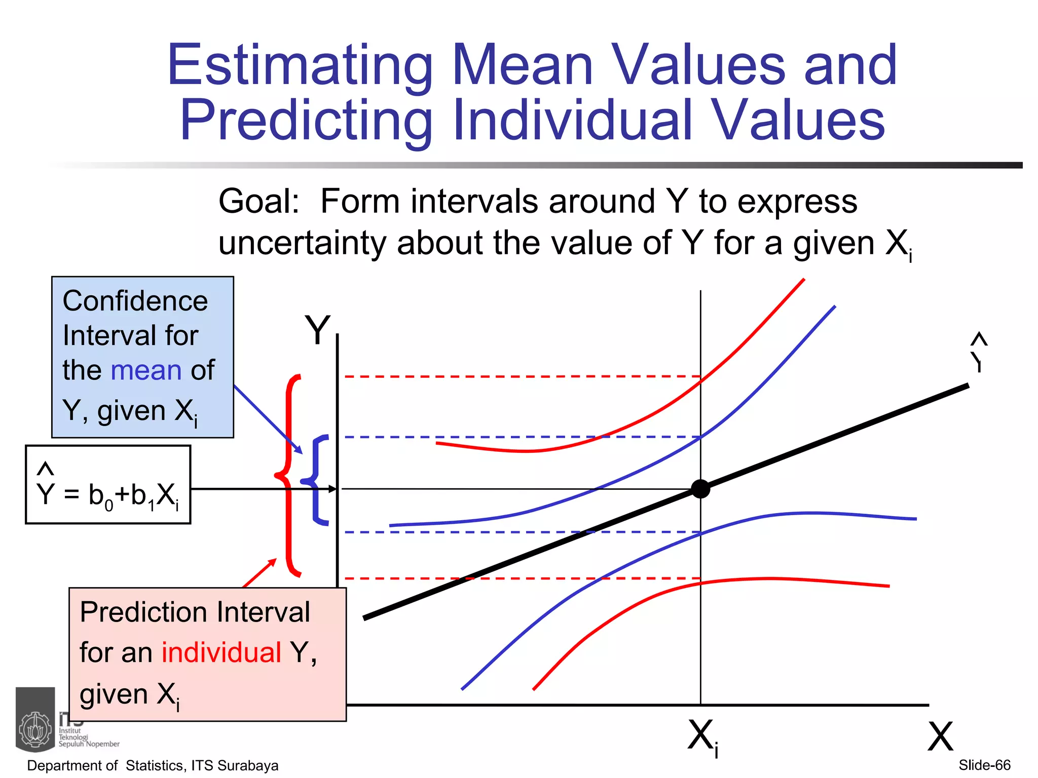
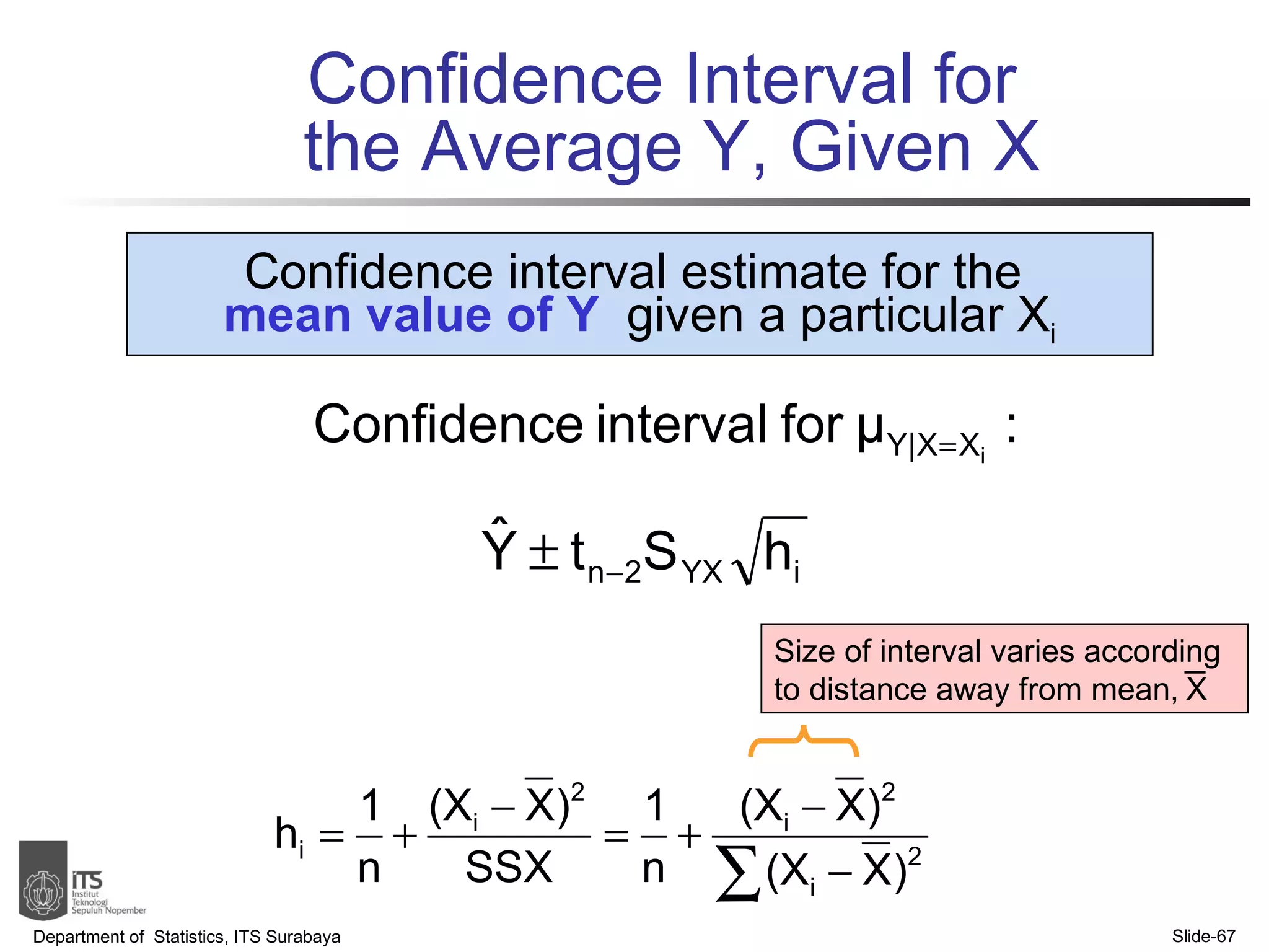
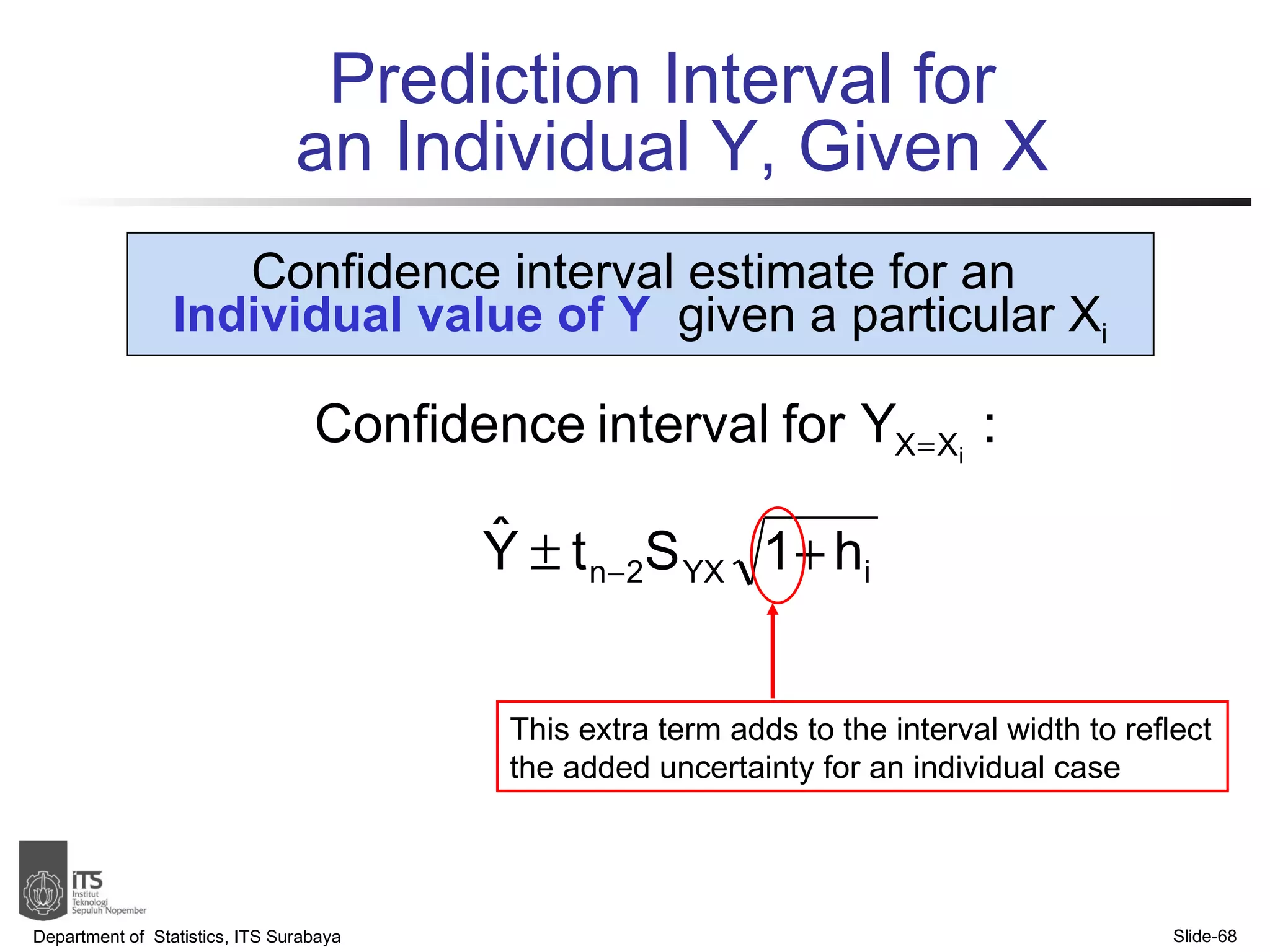
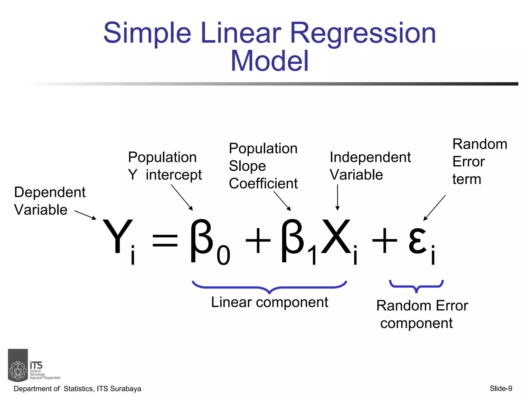
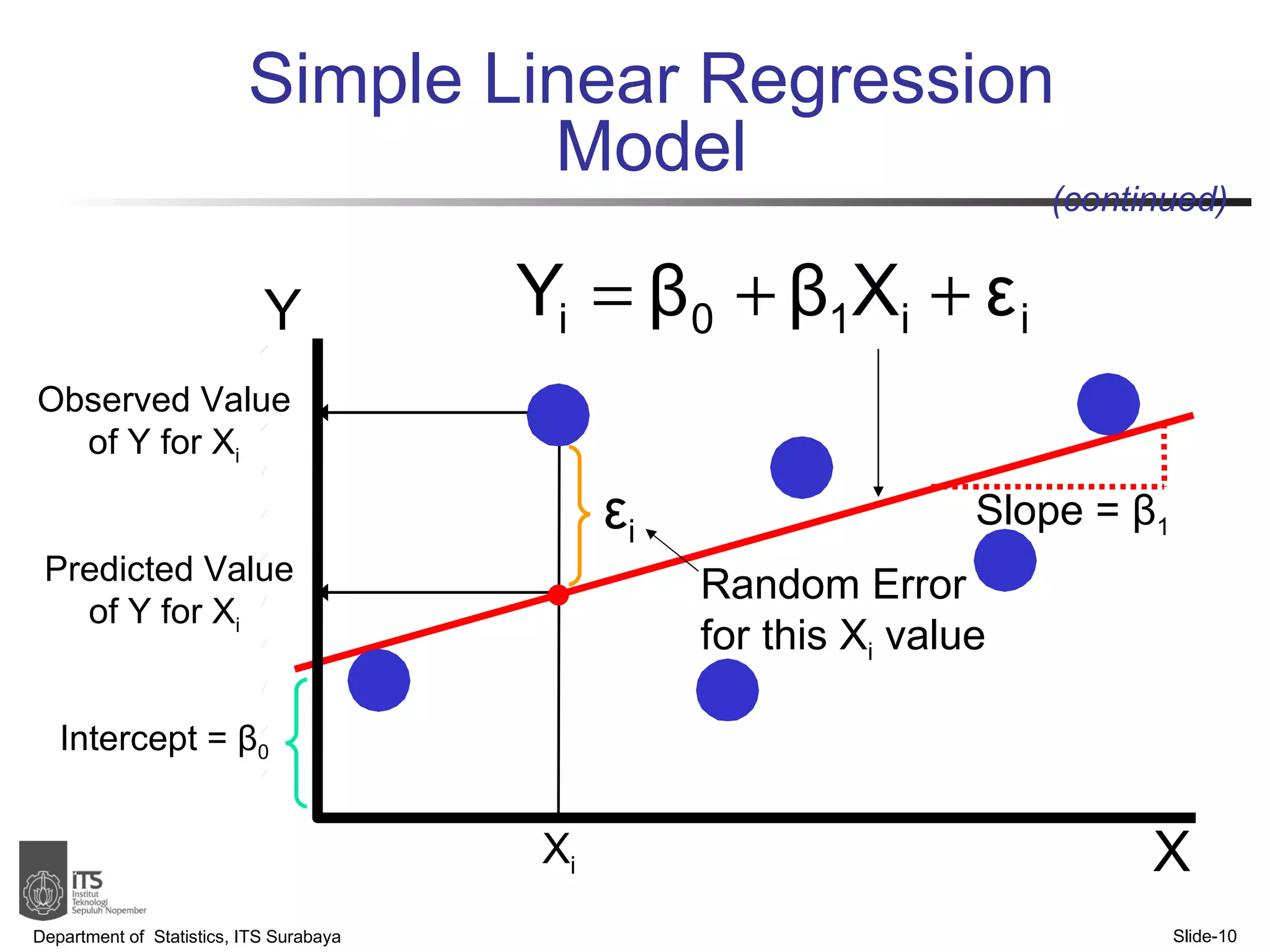
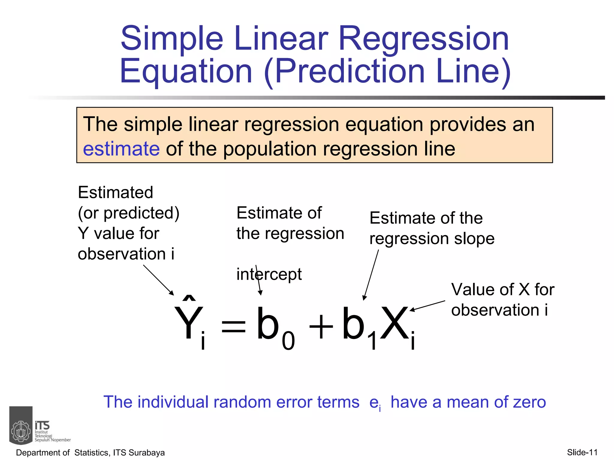
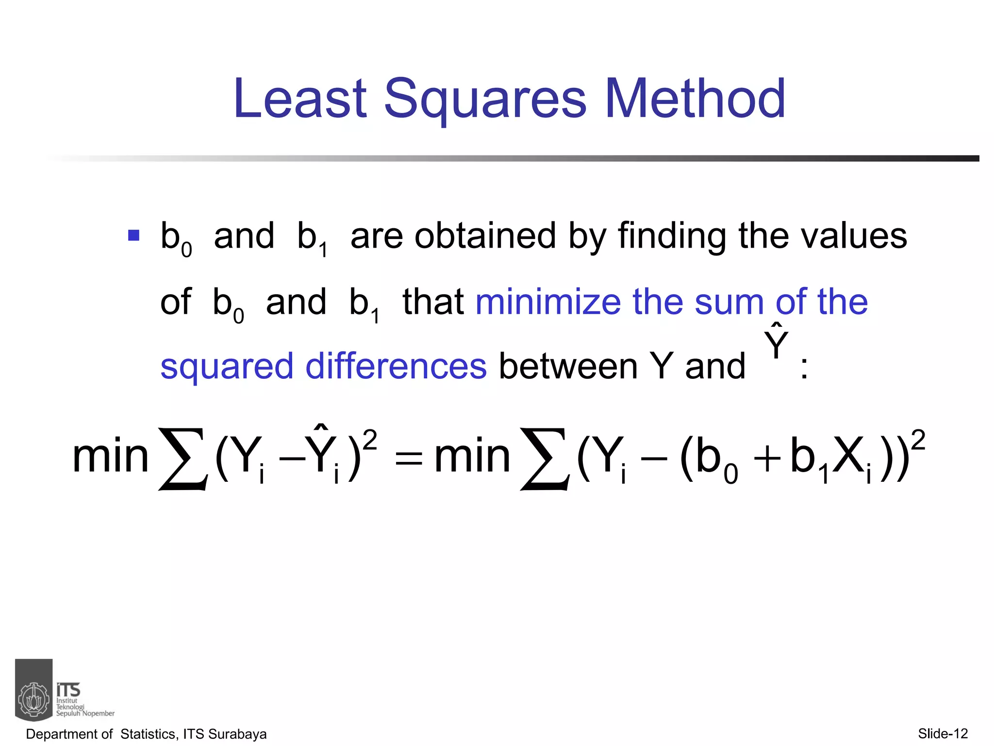
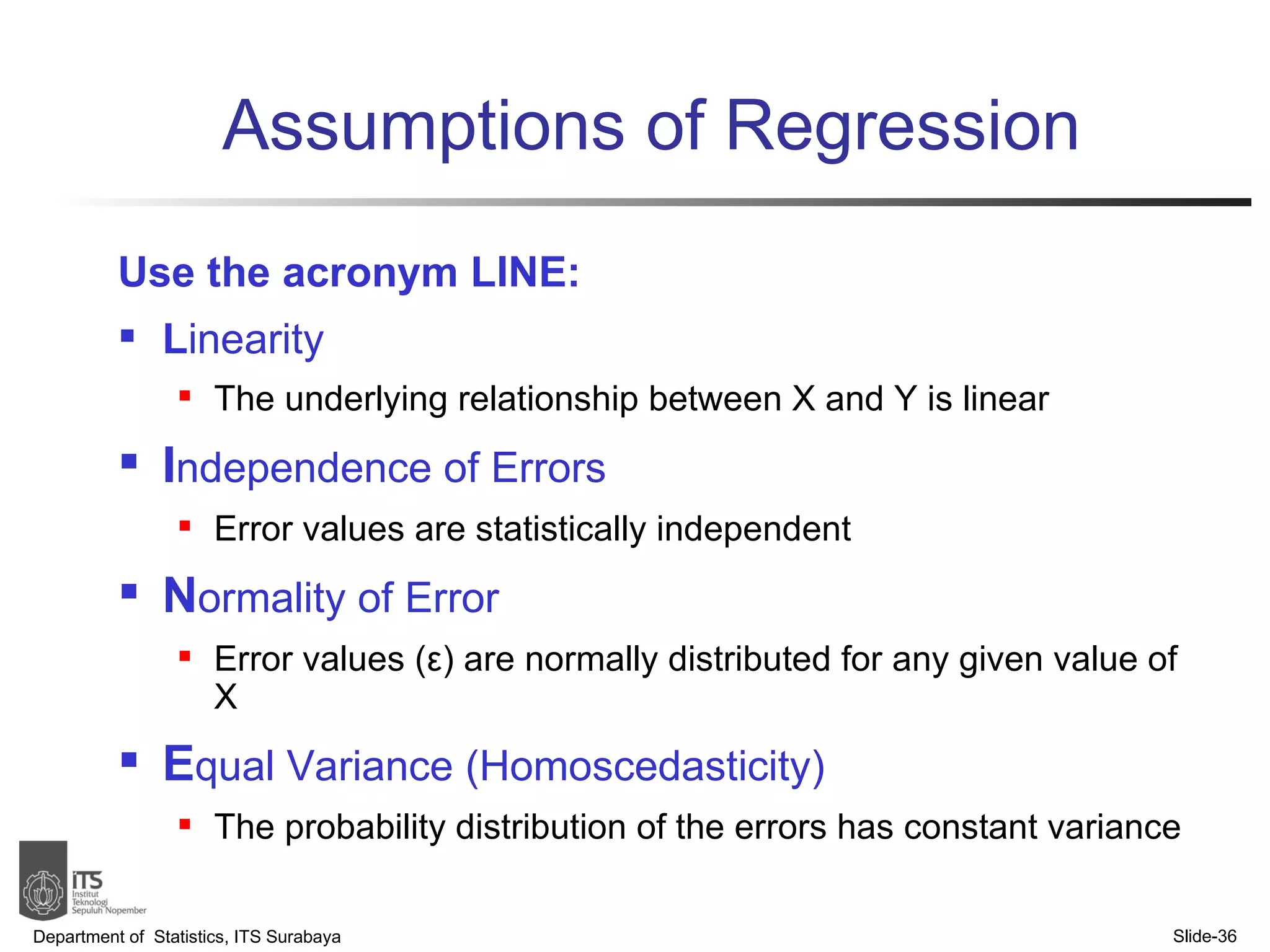
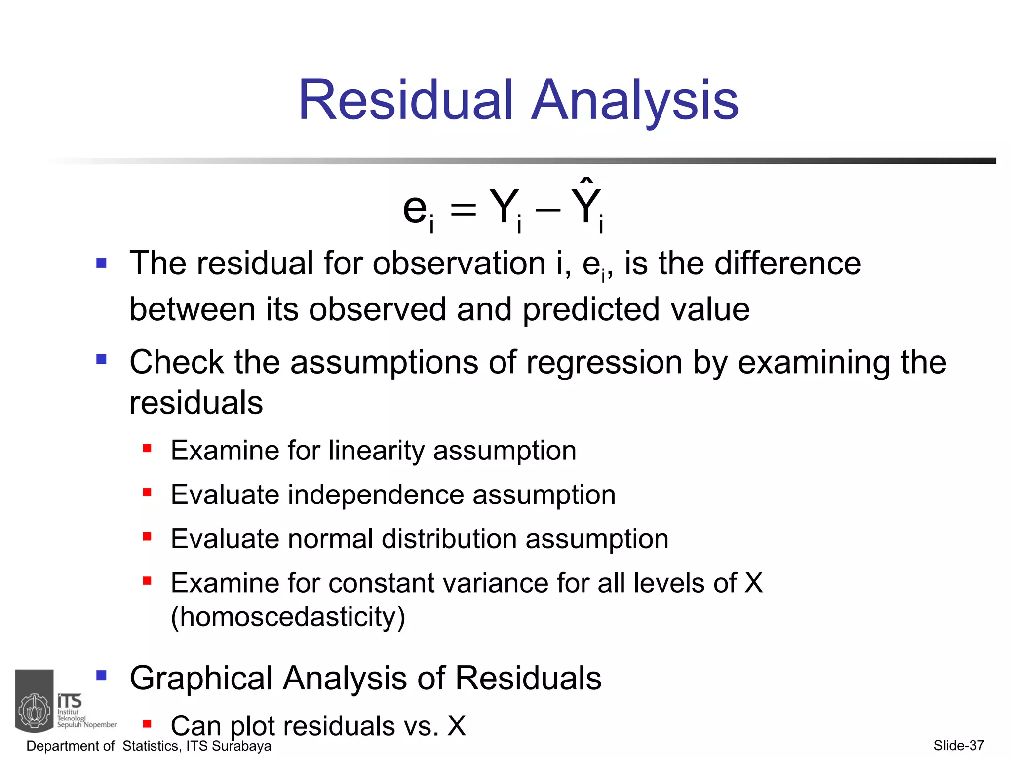
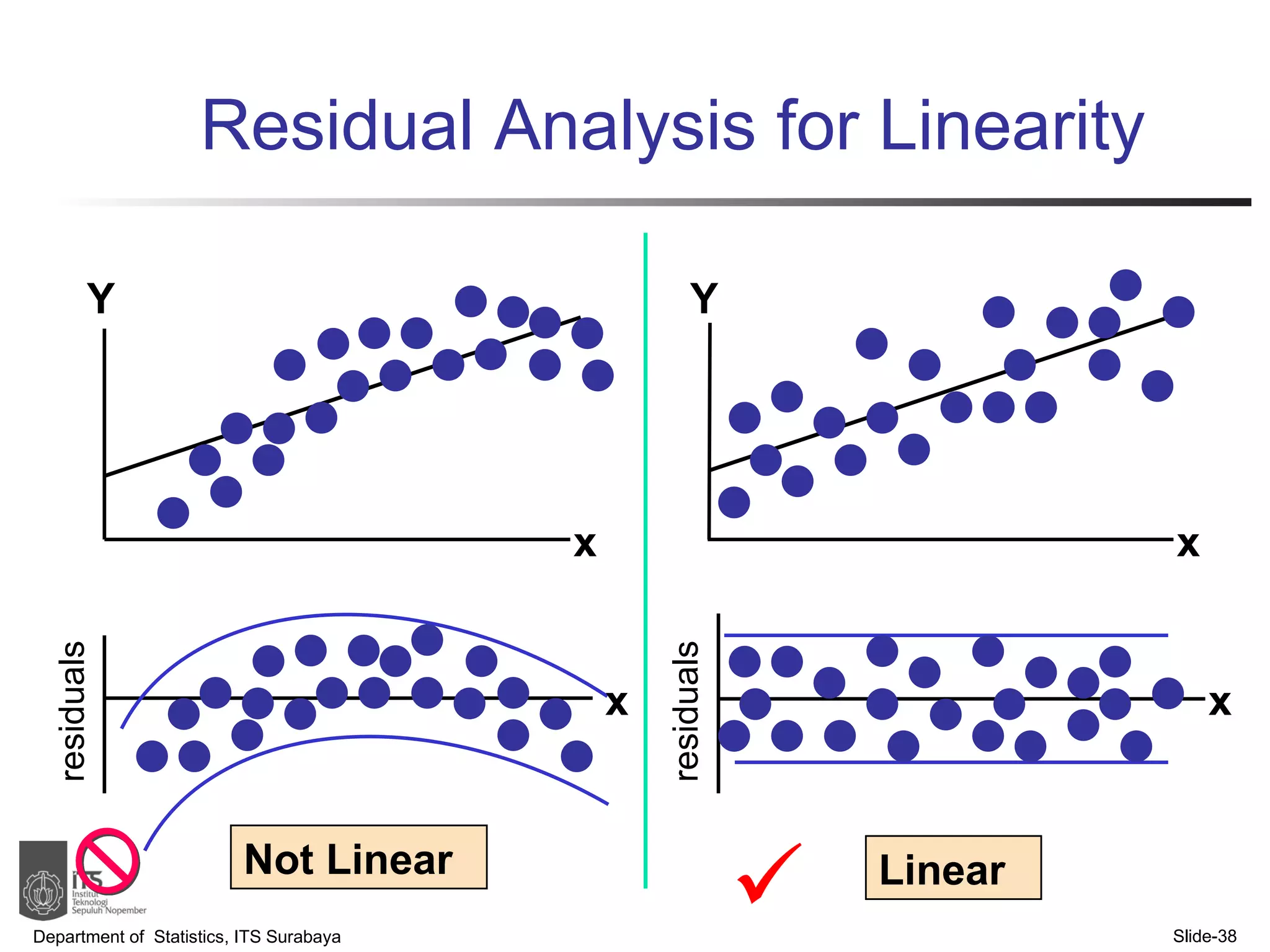
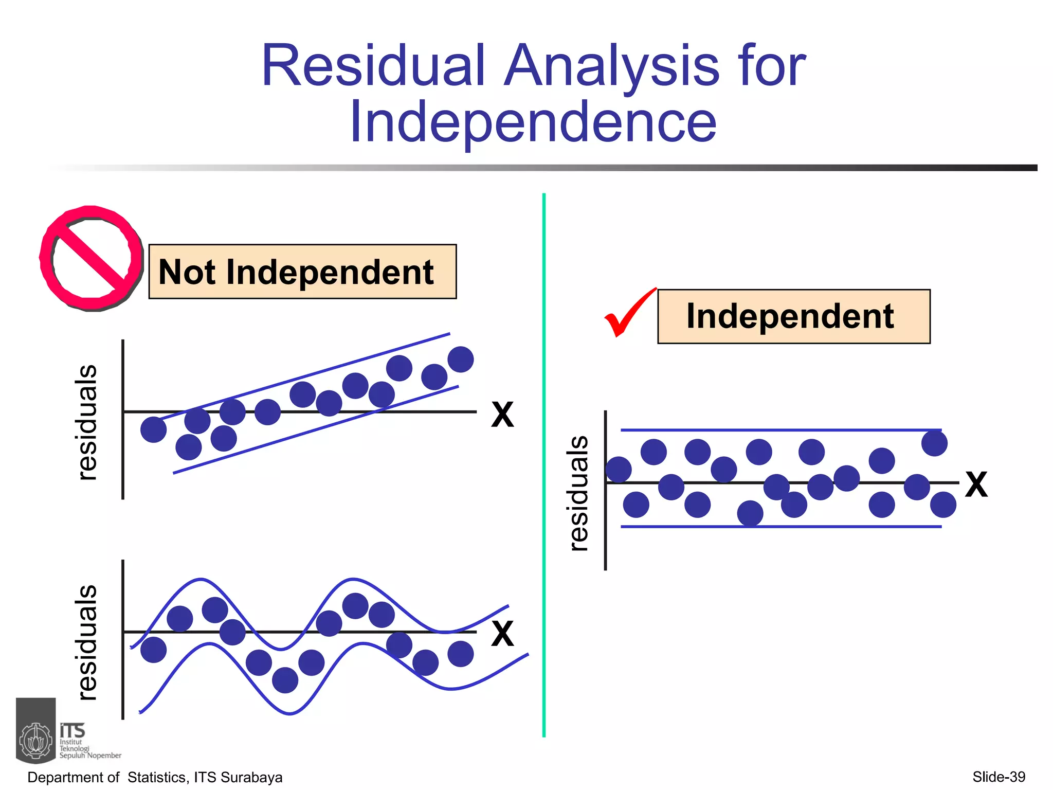
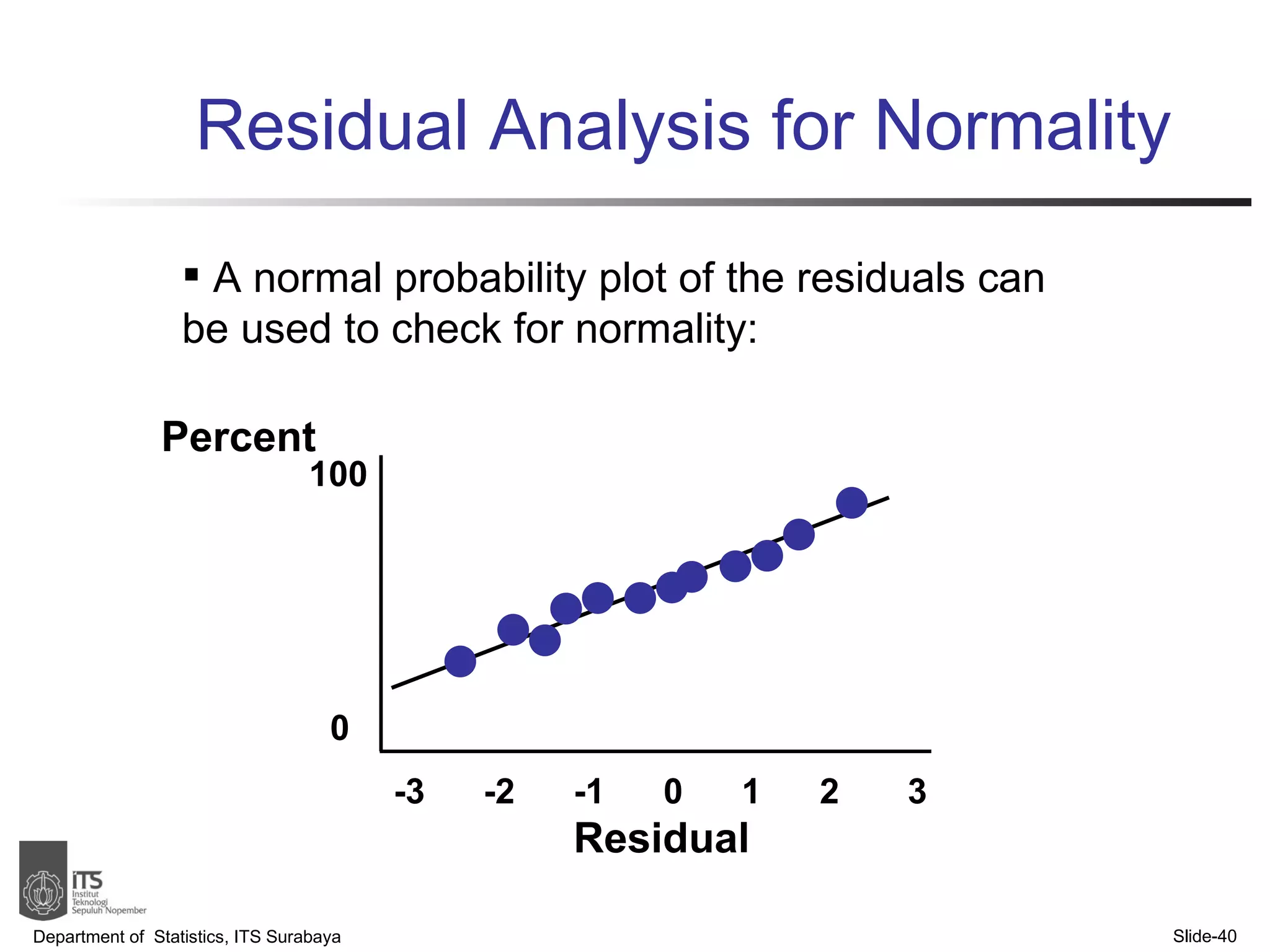
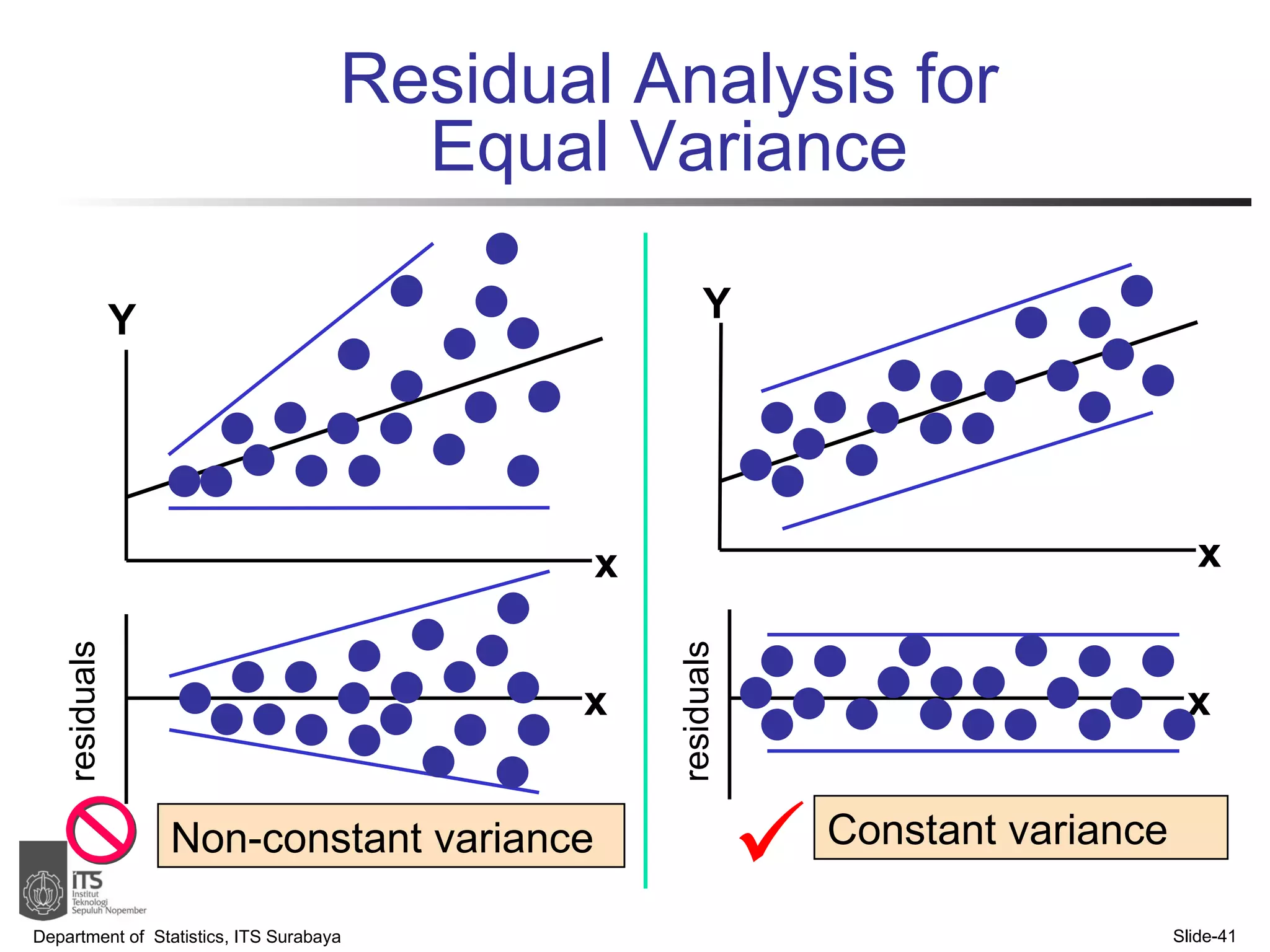
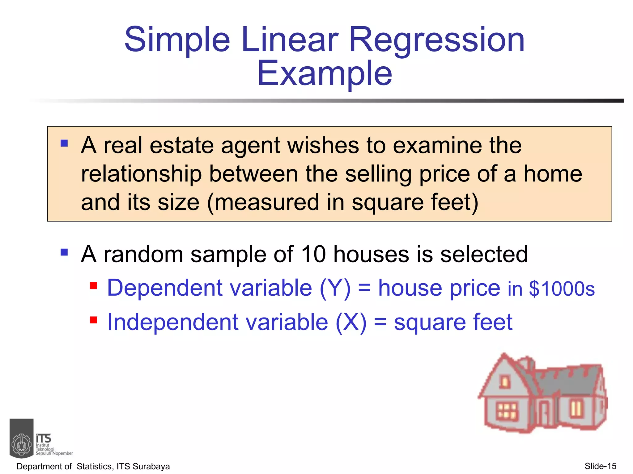
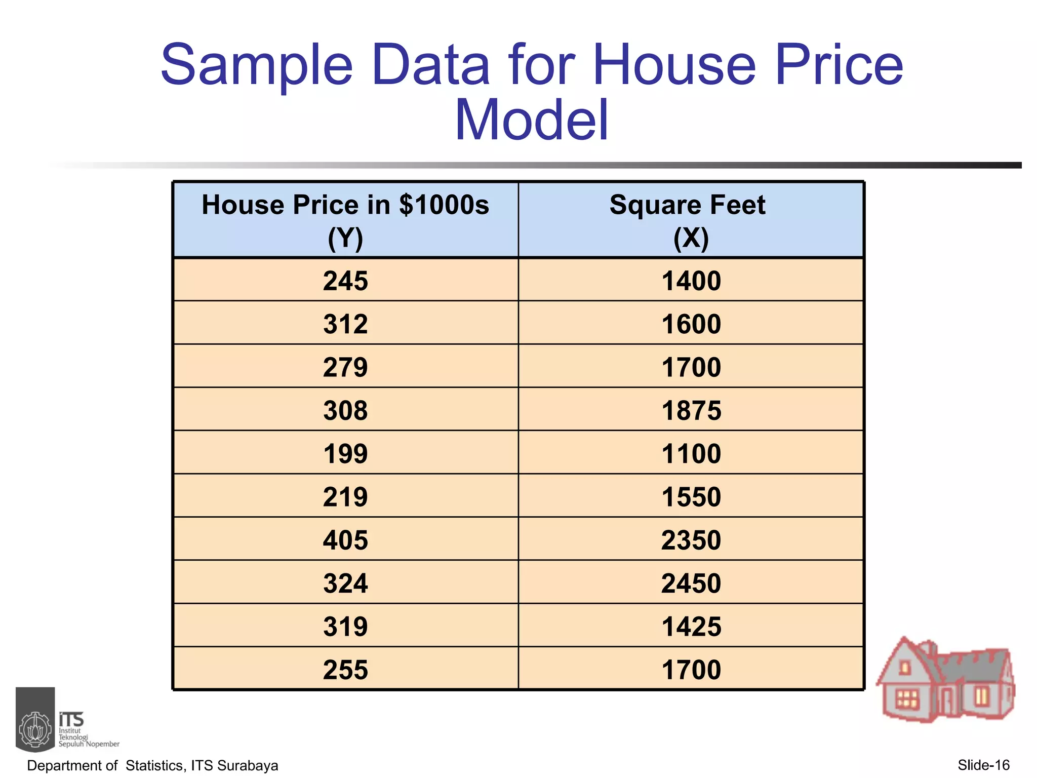
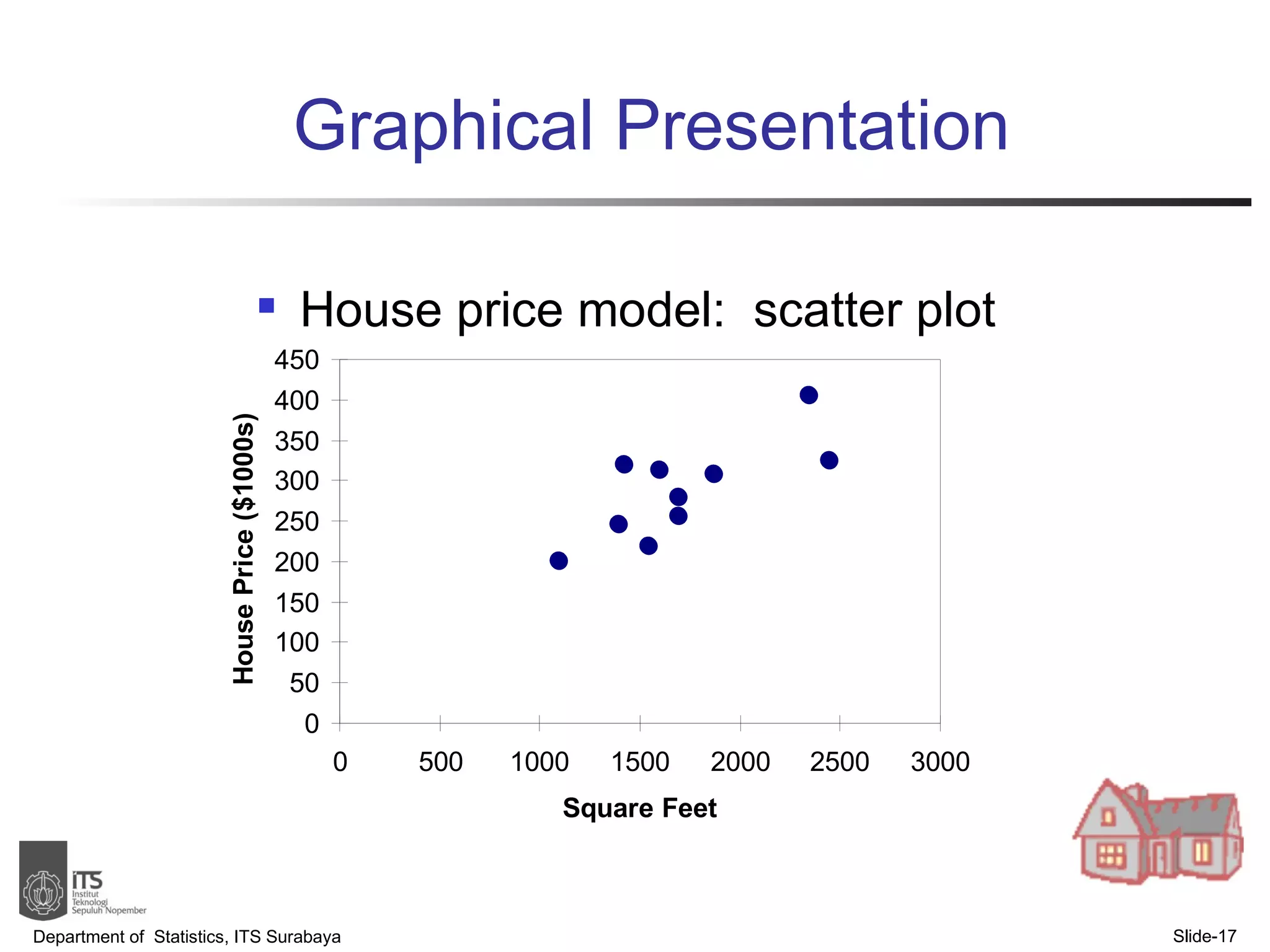
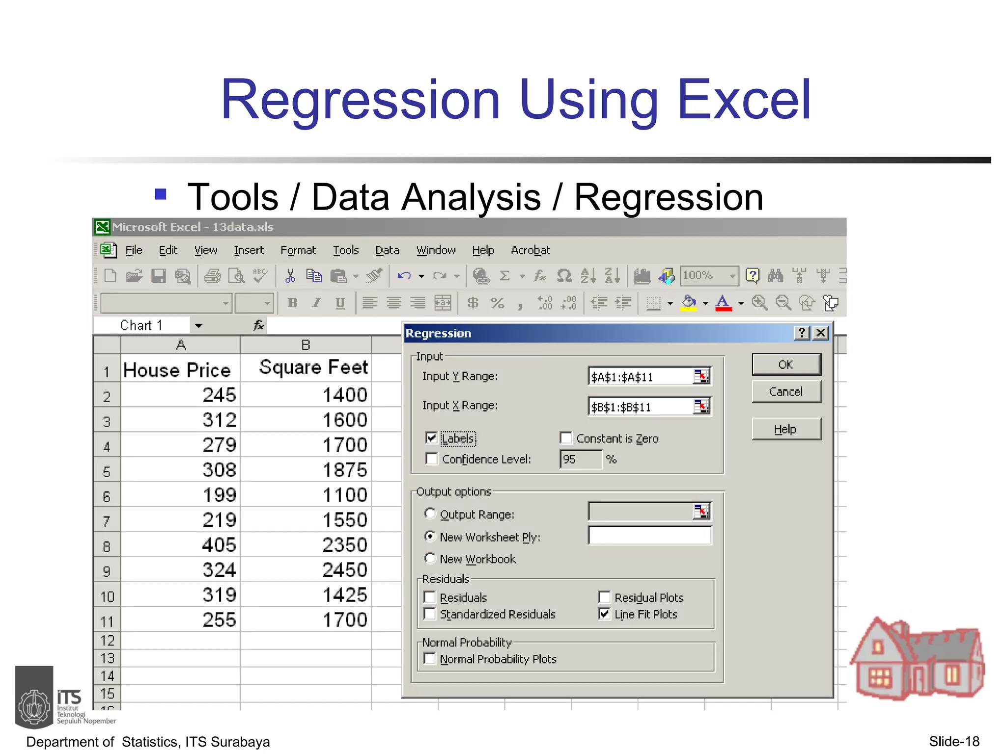
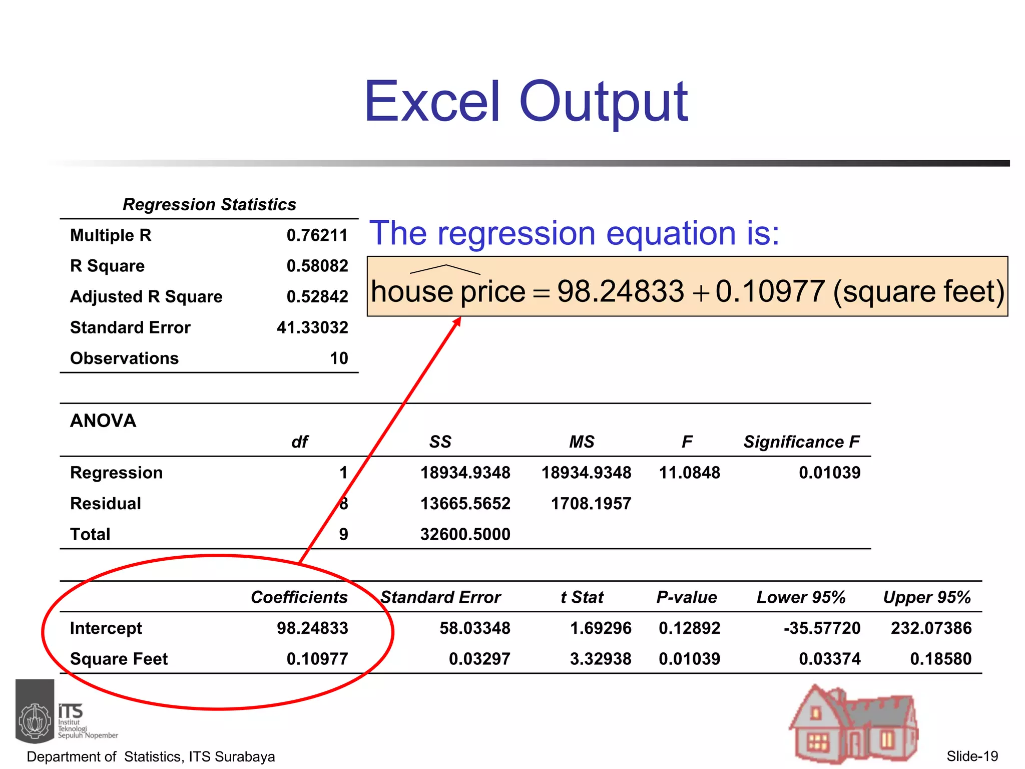
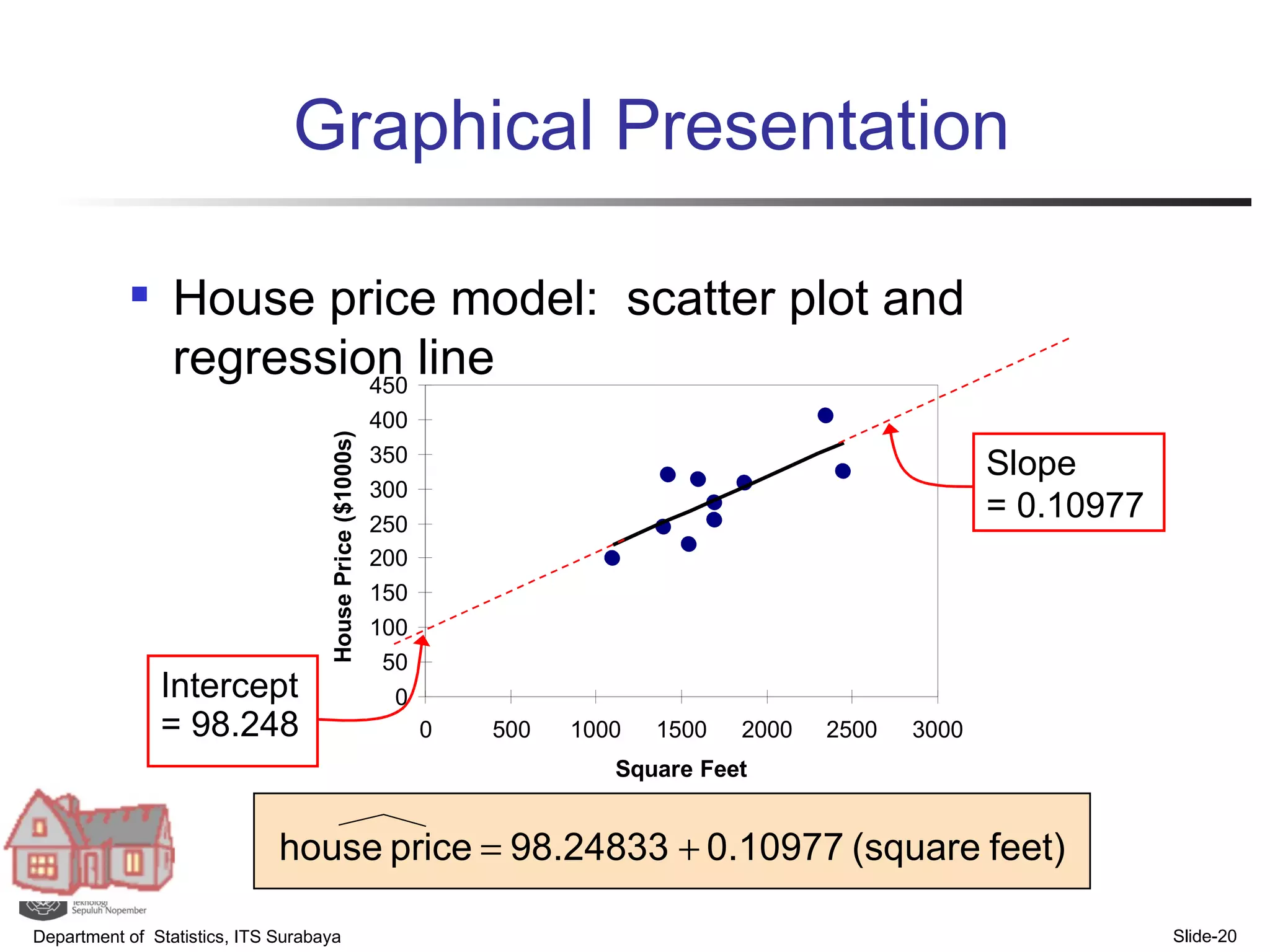
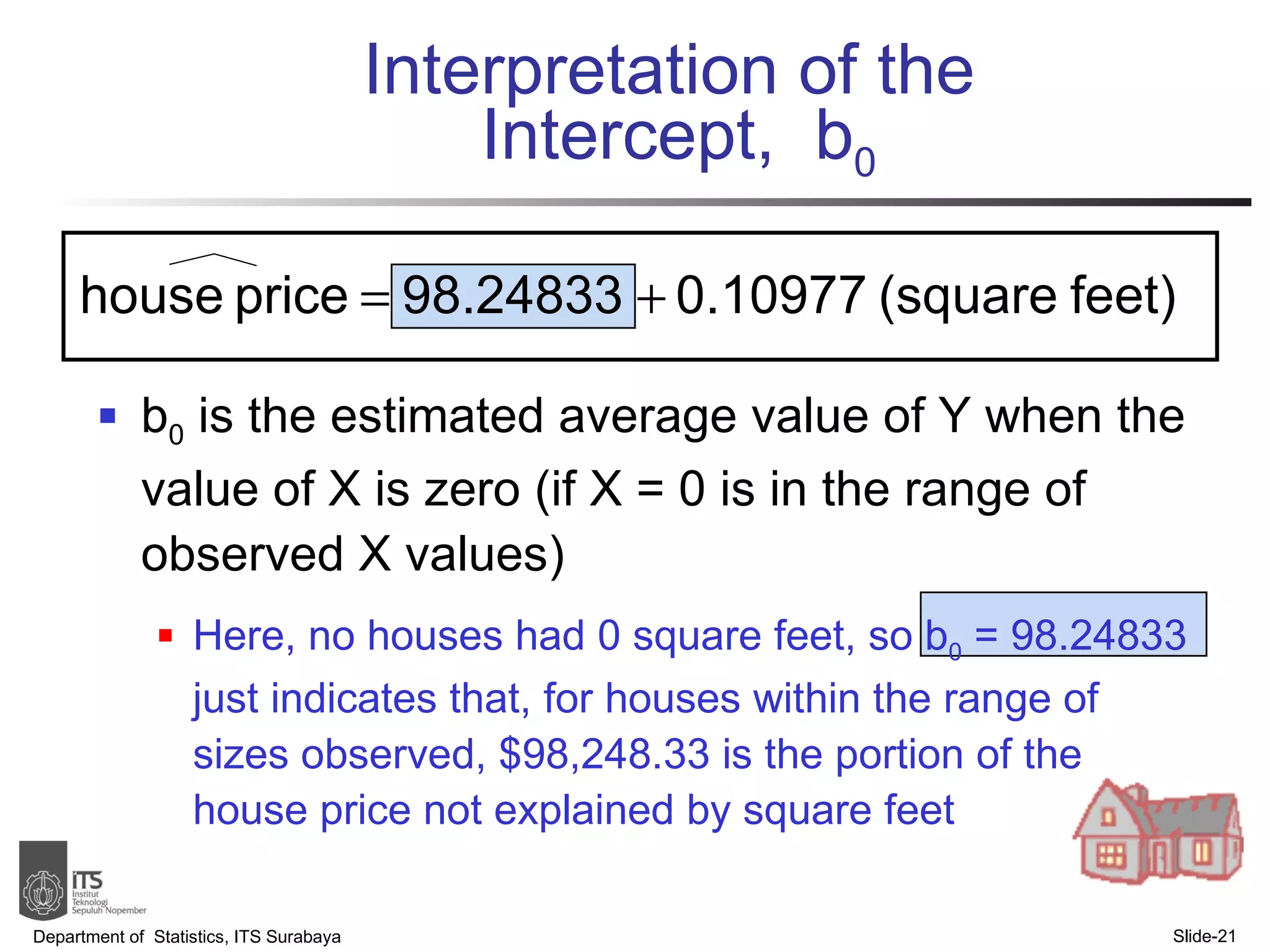
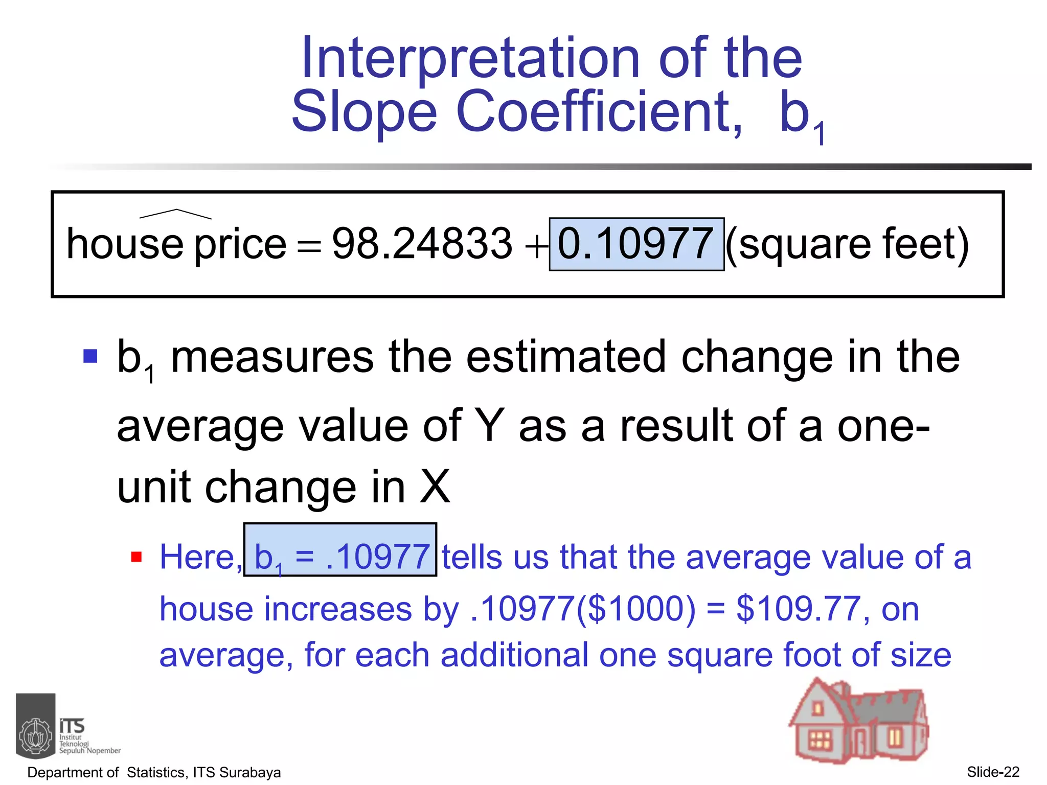
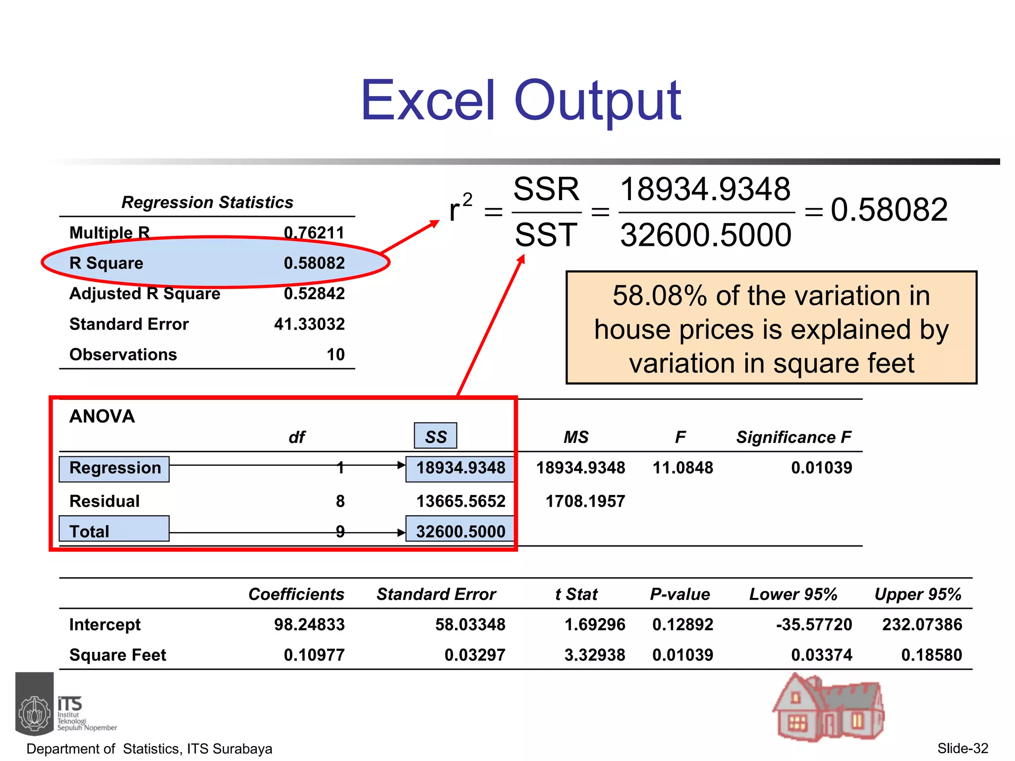
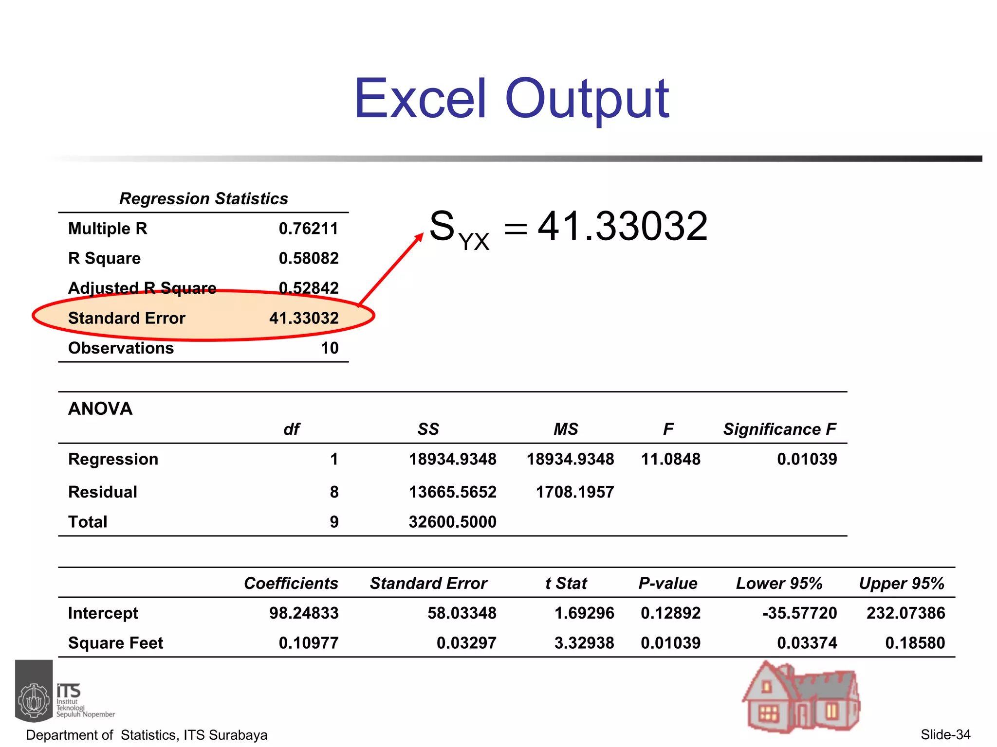
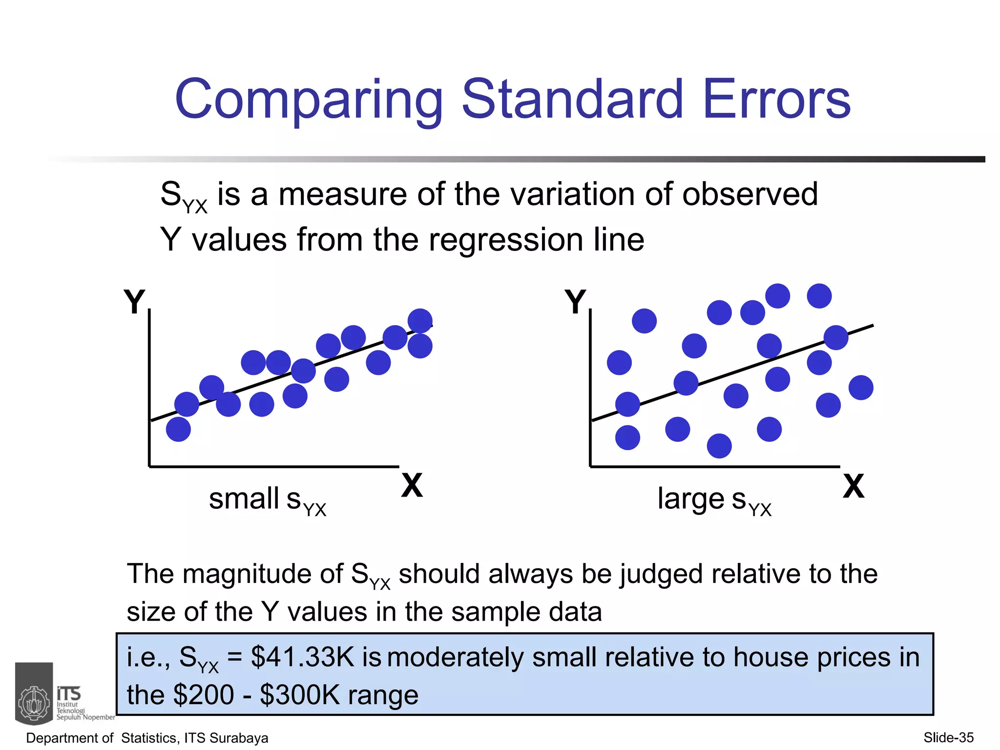
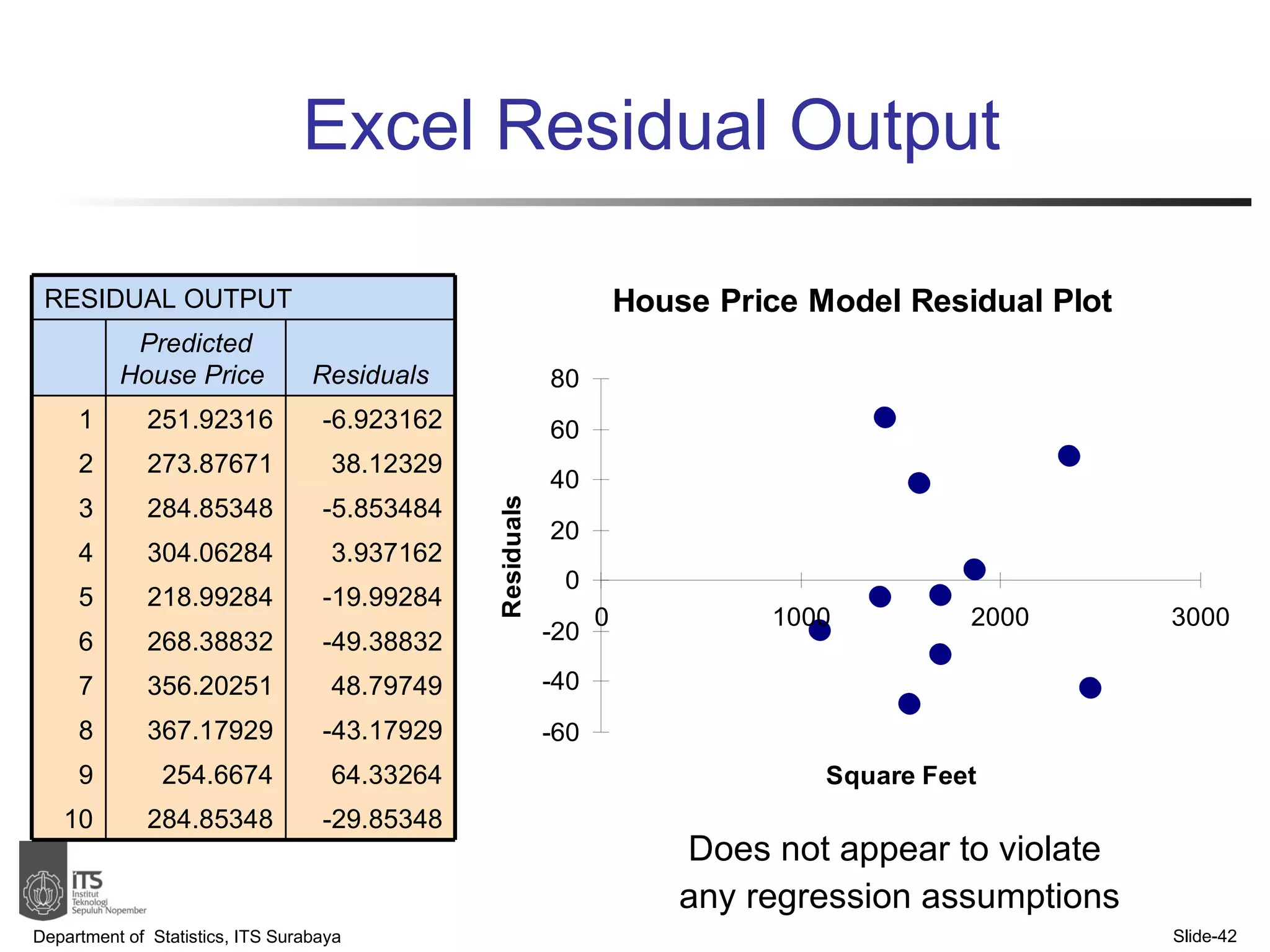
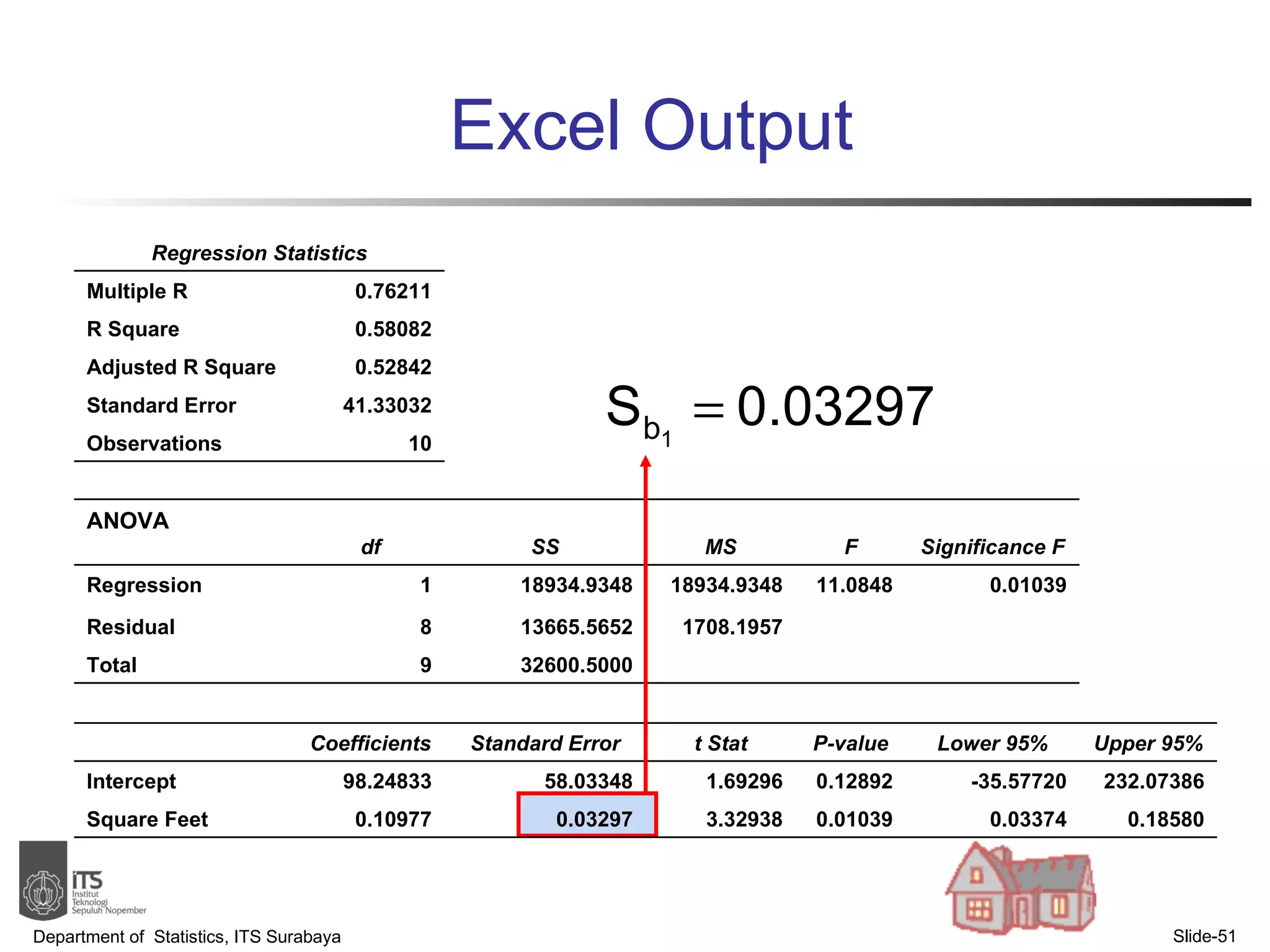
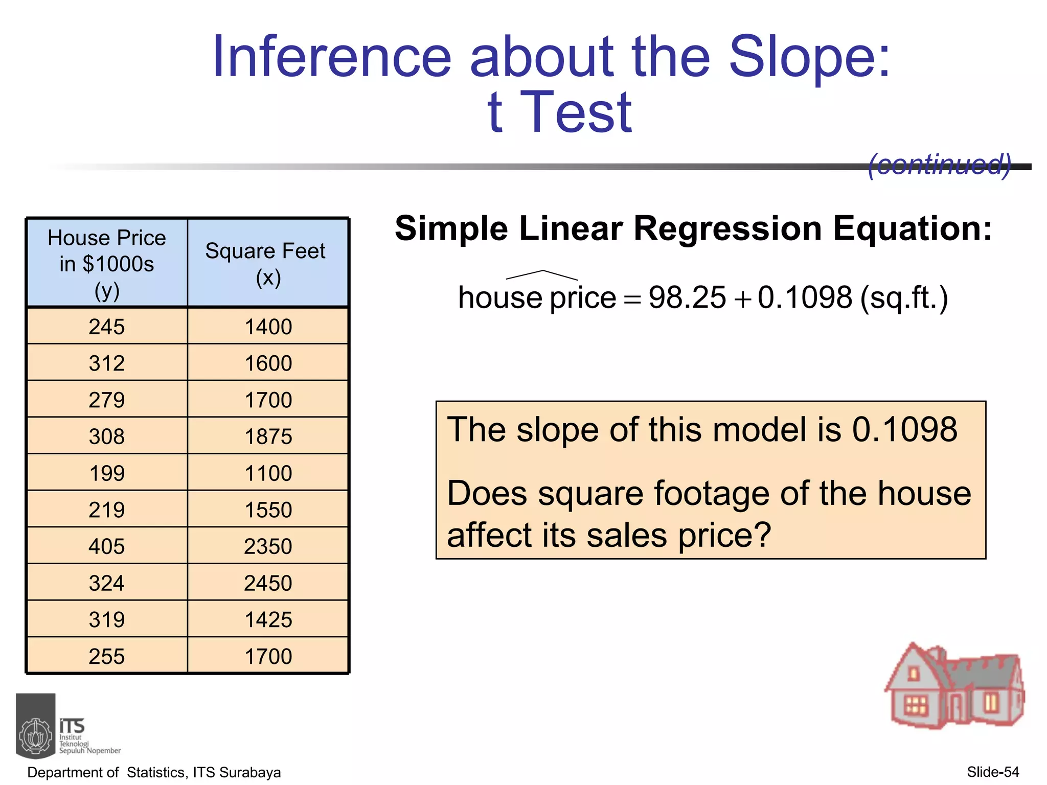
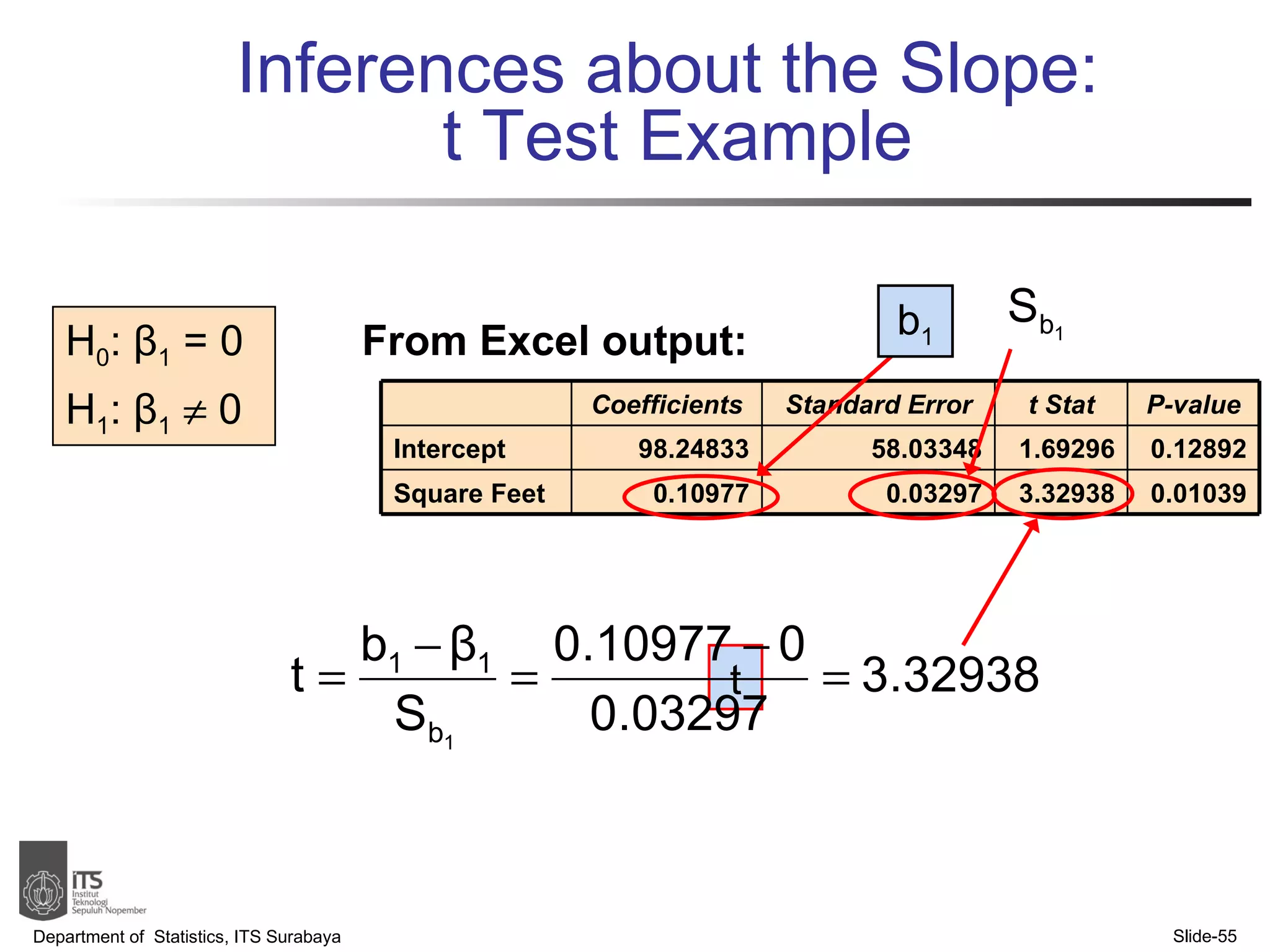
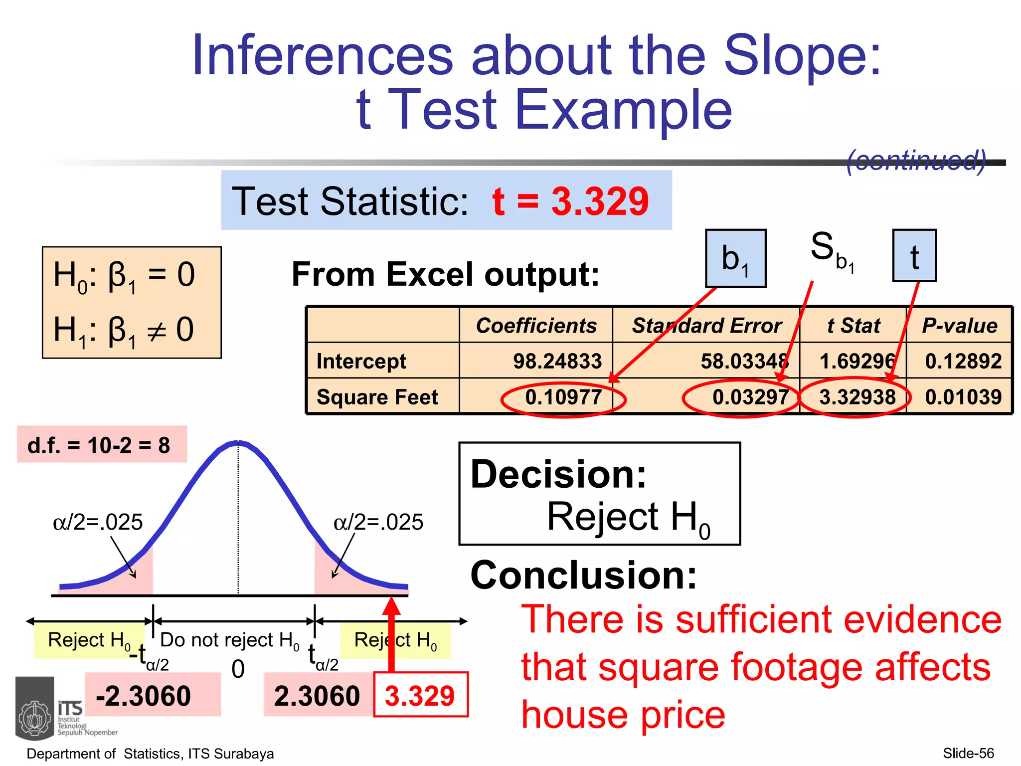
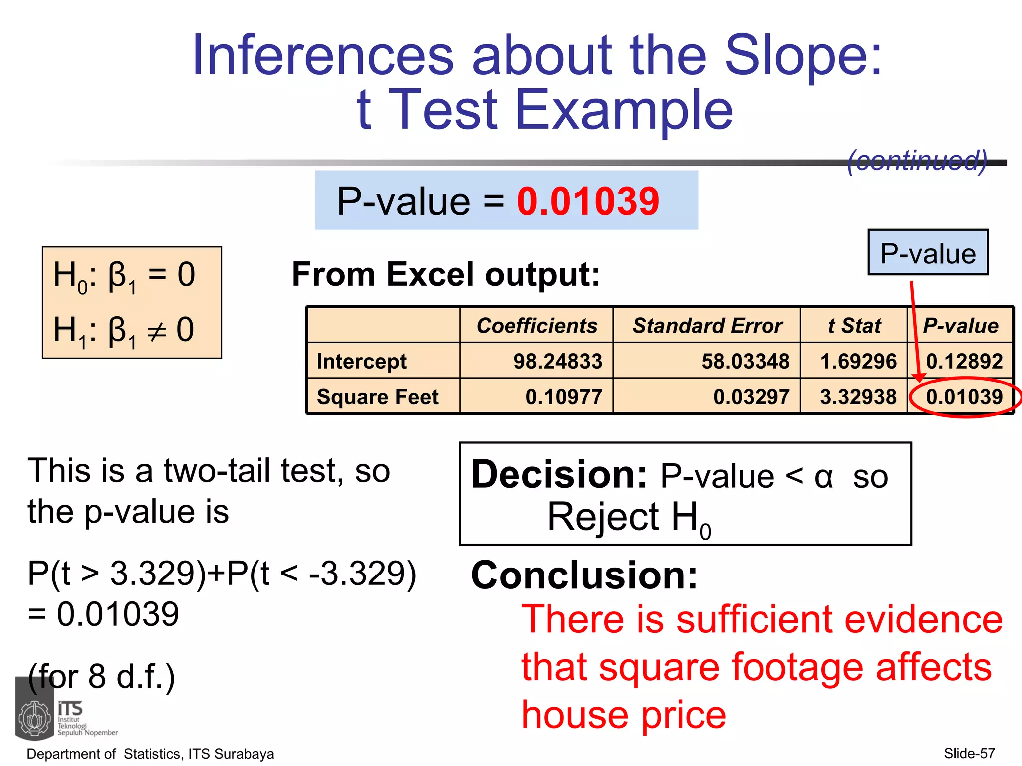
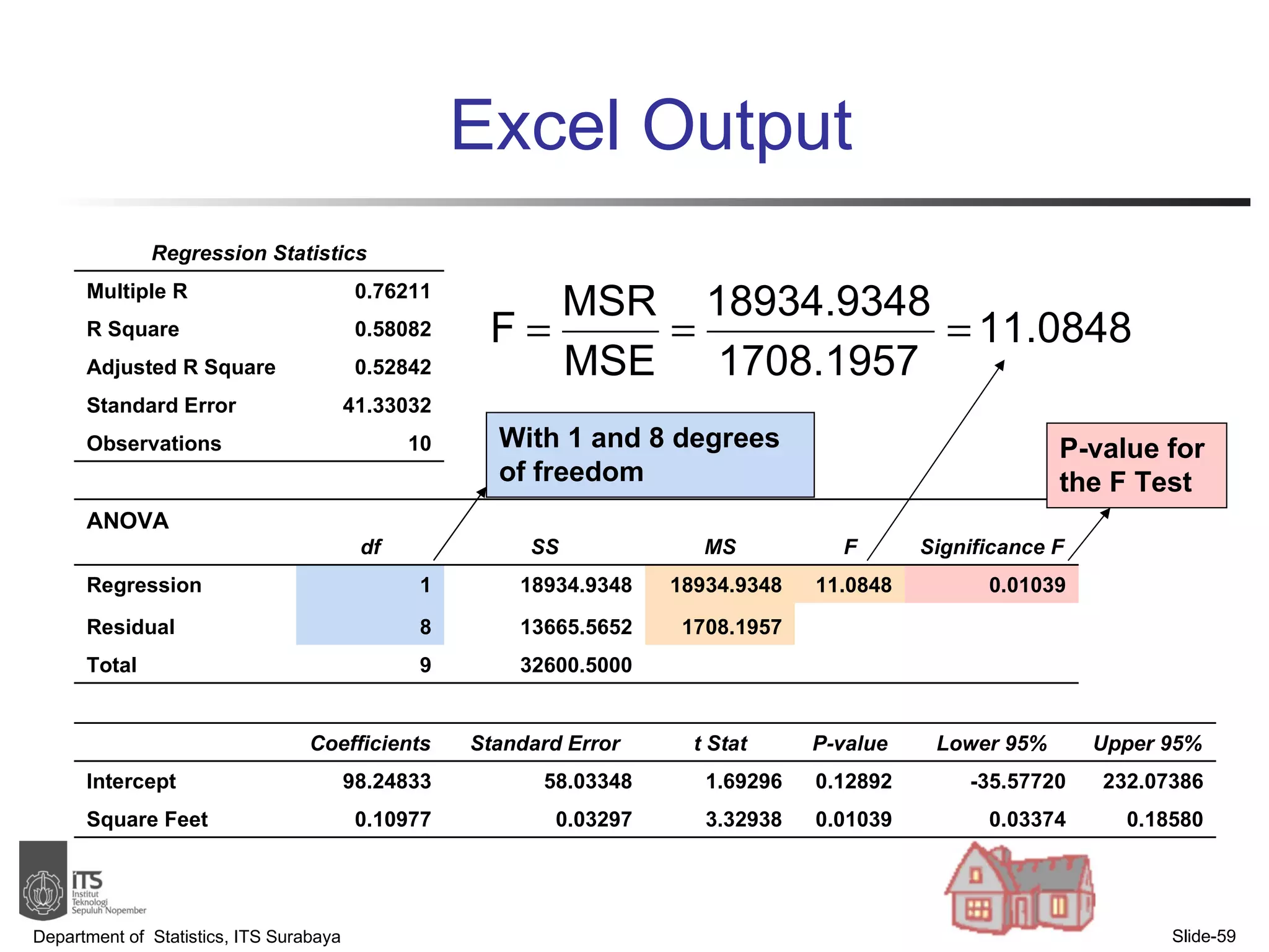
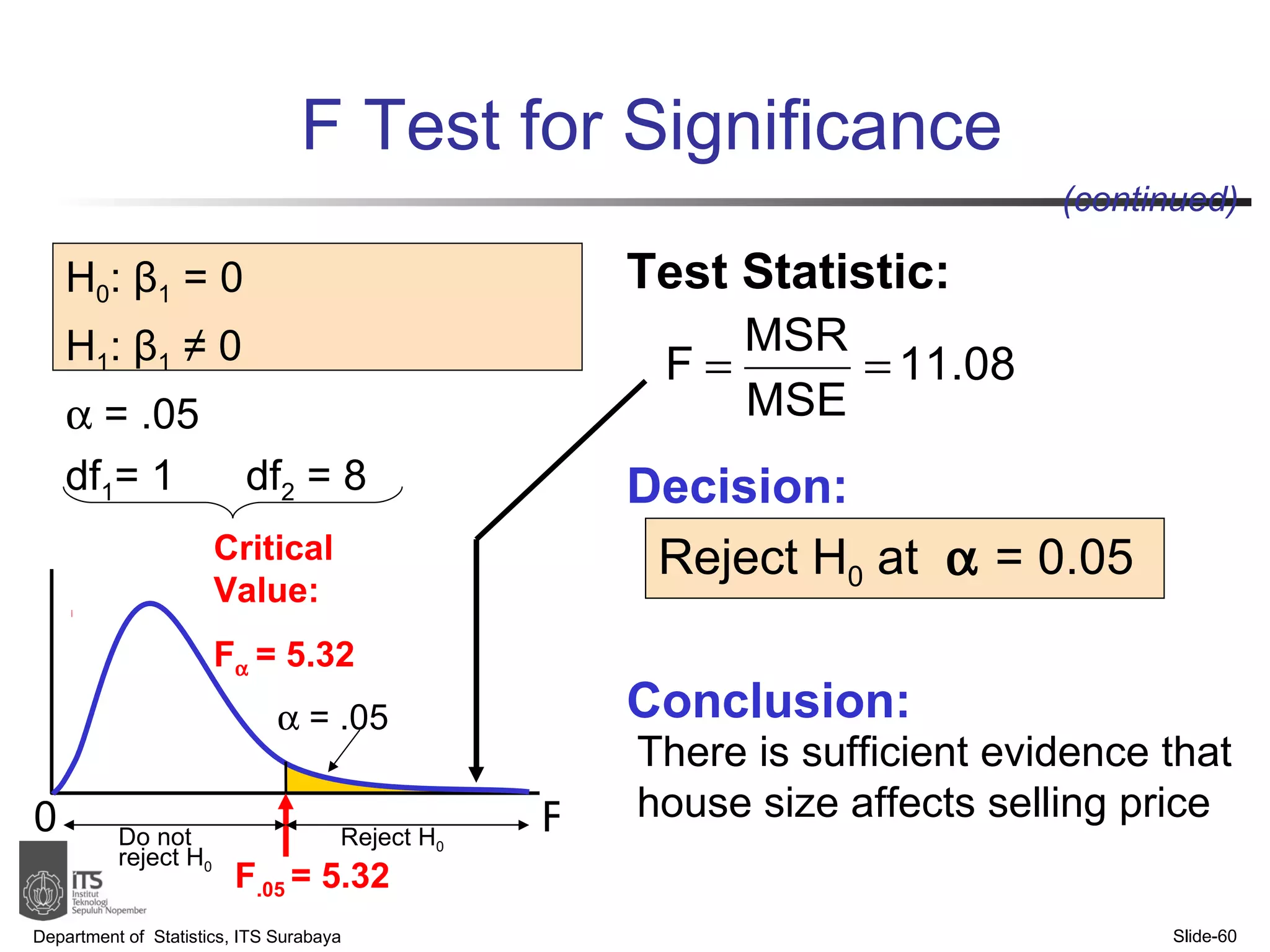
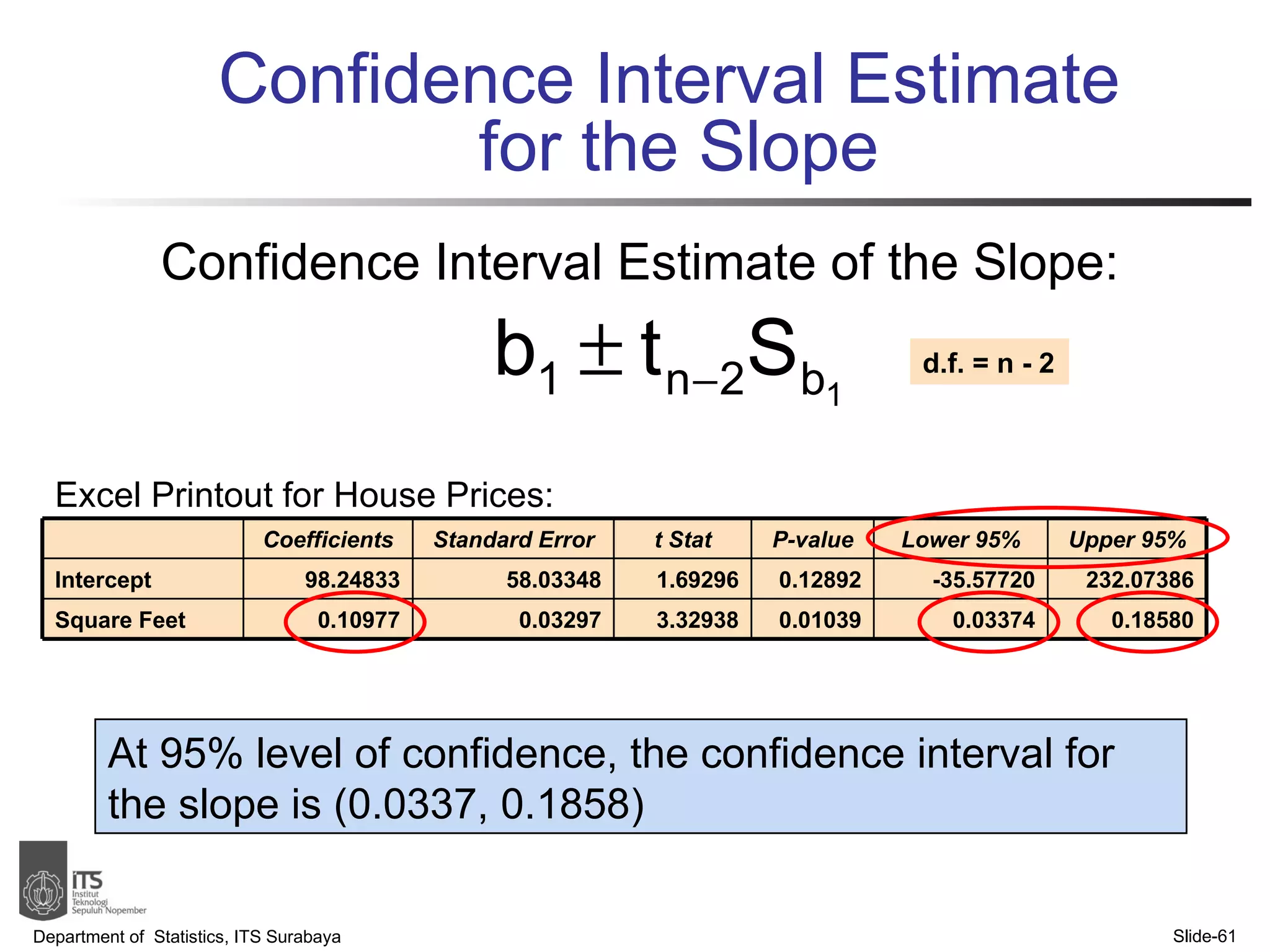
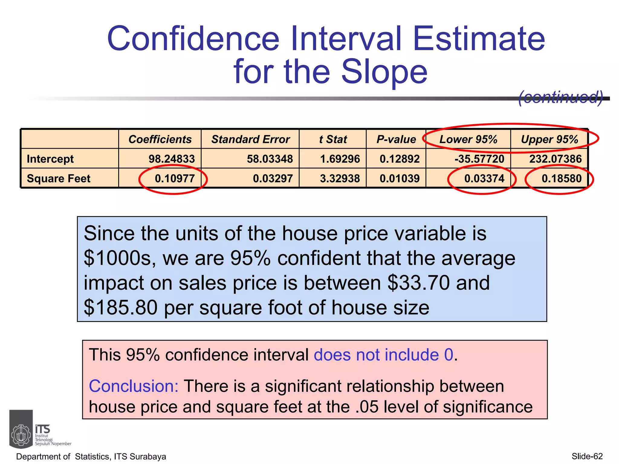
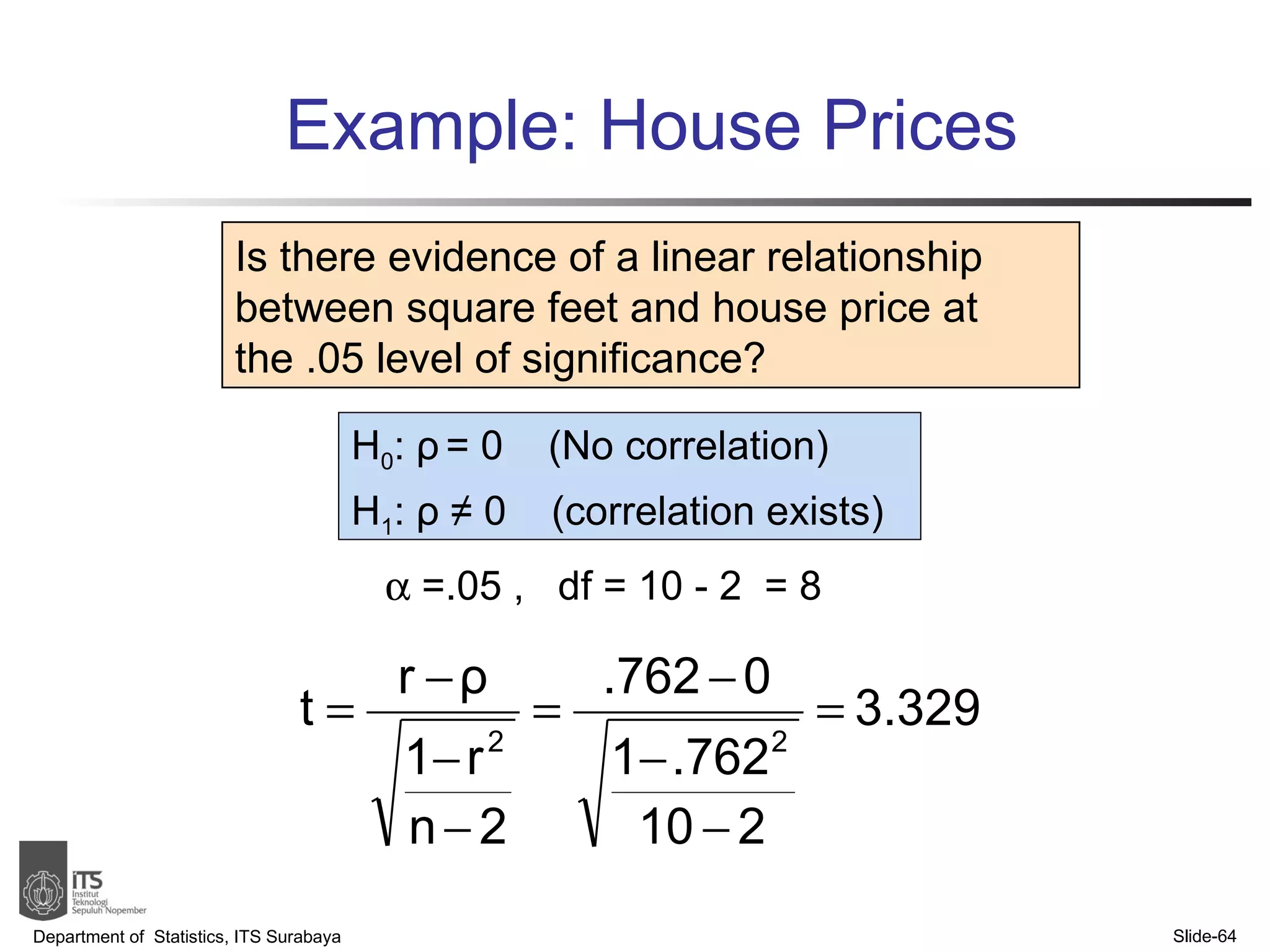
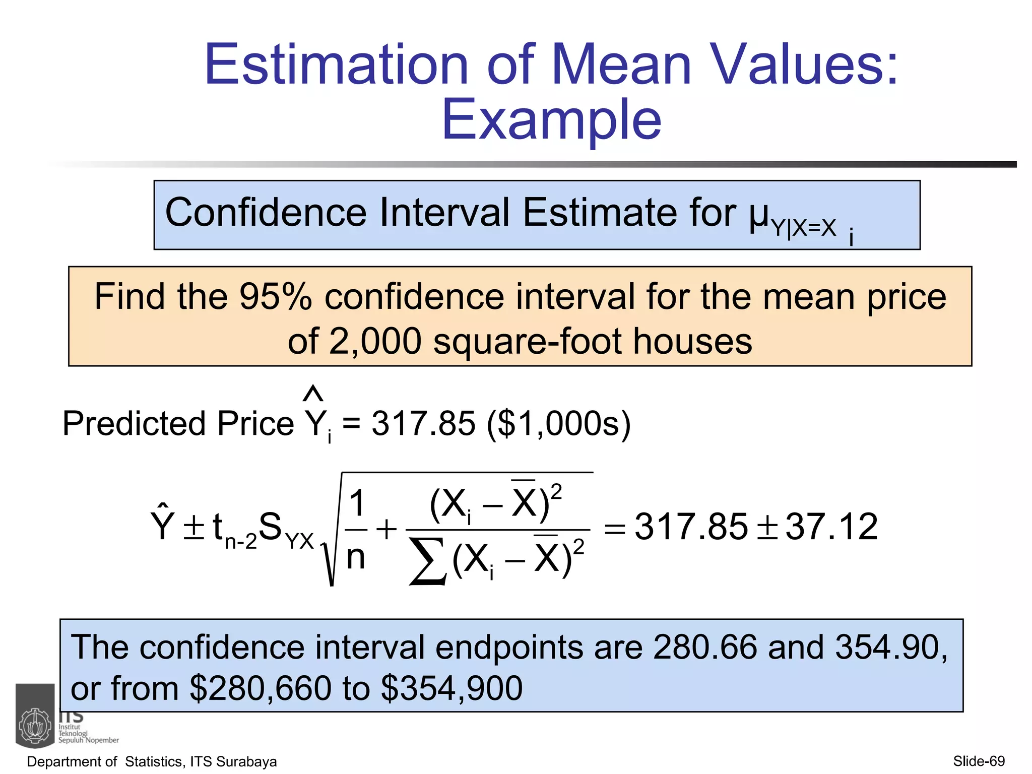
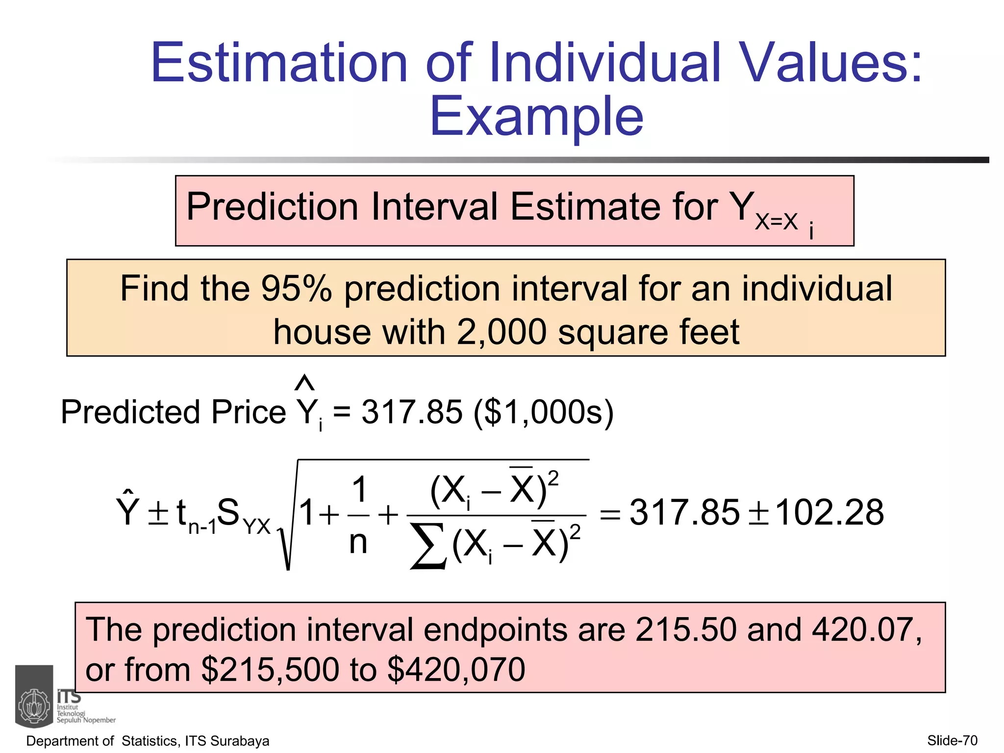
- The document discusses simple linear regression analysis and how to use it to predict a dependent variable (y) based on an independent variable (x). - Key points covered include the simple linear regression model, estimating regression coefficients, evaluating assumptions, making predictions, and interpreting results. - Examples are provided to demonstrate simple linear regression analysis using data on house prices and sizes.

1. Simple Linear Regression Department of Statistics, ITS Surabaya Slide- Prepared by: Sutikno Department of Statistics Faculty of Mathematics and Natural Sciences Sepuluh Nopember Institute of Technology (ITS) Surabaya

2. Learning Objectives How to use regression analysis to predict the value of a dependent variable based on an independent variable The meaning of the regression coefficients b 0 and b 1 How to evaluate the assumptions of regression analysis and know what to do if the assumptions are violated To make inferences about the slope and correlation coefficient To estimate mean values and predict individual values Department of Statistics, ITS Surabaya Slide-

3. Correlation vs. Regression A scatter diagram can be used to show the relationship between two variables Correlation analysis is used to measure strength of the association (linear relationship) between two variables Correlation is only concerned with strength of the relationship No causal effect is implied with correlation Department of Statistics, ITS Surabaya Slide-

4. Introduction to Regression Analysis Regression analysis is used to: Predict the value of a dependent variable based on the value of at least one independent variable Explain the impact of changes in an independent variable on the dependent variable Dependent variable: the variable we wish to predict or explain Independent variable: the variable used to explain the dependent variable Department of Statistics, ITS Surabaya Slide-

5. Simple Linear Regression Model Only one independent variable , X Relationship between X and Y is described by a linear function Changes in Y are assumed to be caused by changes in X Department of Statistics, ITS Surabaya Slide-

6. Types of Relationships Department of Statistics, ITS Surabaya Slide- Y X Y X Y Y X X Linear relationships Curvilinear relationships

7. Types of Relationships Department of Statistics, ITS Surabaya Slide- Y X Y X Y Y X X Strong relationships Weak relationships (continued)

8. Types of Relationships Department of Statistics, ITS Surabaya Slide- Y X Y X No relationship (continued)

9. Simple Linear Regression Model Department of Statistics, ITS Surabaya Slide- Linear component Population Y intercept Population Slope Coefficient Random Error term Dependent Variable Independent Variable Random Error component

10. Simple Linear Regression Model Department of Statistics, ITS Surabaya Slide- (continued) Random Error for this X i value Y X Observed Value of Y for X i Predicted Value of Y for X i X i Slope = β 1 Intercept = β 0 ε i

11. Simple Linear Regression Equation (Prediction Line) Department of Statistics, ITS Surabaya Slide- The simple linear regression equation provides an estimate of the population regression line Estimate of the regression intercept Estimate of the regression slope Estimated (or predicted) Y value for observation i Value of X for observation i The individual random error terms e i have a mean of zero

12. Least Squares Method b 0 and b 1 are obtained by finding the values of b 0 and b 1 that minimize the sum of the squared differences between Y and : Department of Statistics, ITS Surabaya Slide-

13. Finding the Least Squares Equation The coefficients b 0 and b 1 , and other regression results in this section, will be found using Excel or SPSS Department of Statistics, ITS Surabaya Slide- Formulas are shown in the text for those who are interested

14. b 0 is the estimated average value of Y when the value of X is zero b 1 is the estimated change in the average value of Y as a result of a one-unit change in X Interpretation of the Slope and the Intercept Department of Statistics, ITS Surabaya Slide-

15. Simple Linear Regression Example A real estate agent wishes to examine the relationship between the selling price of a home and its size (measured in square feet) A random sample of 10 houses is selected Dependent variable (Y) = house price in $1000s Independent variable (X) = square feet Department of Statistics, ITS Surabaya Slide-

16. Sample Data for House Price Model Department of Statistics, ITS Surabaya Slide- House Price in $1000s (Y) Square Feet (X) 245 1400 312 1600 279 1700 308 1875 199 1100 219 1550 405 2350 324 2450 319 1425 255 1700

17. Graphical Presentation House price model: scatter plot Department of Statistics, ITS Surabaya Slide-

18. Regression Using Excel Tools / Data Analysis / Regression Department of Statistics, ITS Surabaya Slide-

19. Excel Output Department of Statistics, ITS Surabaya Slide- The regression equation is: Regression Statistics Multiple R 0.76211 R Square 0.58082 Adjusted R Square 0.52842 Standard Error 41.33032 Observations 10 ANOVA df SS MS F Significance F Regression 1 18934.9348 18934.9348 11.0848 0.01039 Residual 8 13665.5652 1708.1957 Total 9 32600.5000 Coefficients Standard Error t Stat P-value Lower 95% Upper 95% Intercept 98.24833 58.03348 1.69296 0.12892 -35.57720 232.07386 Square Feet 0.10977 0.03297 3.32938 0.01039 0.03374 0.18580

20. Graphical Presentation House price model: scatter plot and regression line Department of Statistics, ITS Surabaya Slide- Slope = 0.10977 Intercept = 98.248

21. Interpretation of the Intercept, b 0 b 0 is the estimated average value of Y when the value of X is zero (if X = 0 is in the range of observed X values) Here, no houses had 0 square feet, so b 0 = 98.24833 just indicates that, for houses within the range of sizes observed, $98,248.33 is the portion of the house price not explained by square feet Department of Statistics, ITS Surabaya Slide-

22. Interpretation of the Slope Coefficient, b 1 b 1 measures the estimated change in the average value of Y as a result of a one-unit change in X Here, b 1 = .10977 tells us that the average value of a house increases by .10977($1000) = $109.77, on average, for each additional one square foot of size Department of Statistics, ITS Surabaya Slide-

23. Predictions using Regression Analysis Department of Statistics, ITS Surabaya Slide- Predict the price for a house with 2000 square feet: The predicted price for a house with 2000 square feet is 317.85($1,000s) = $317,850

24. Interpolation vs. Extrapolation When using a regression model for prediction, only predict within the relevant range of data Department of Statistics, ITS Surabaya Slide- Relevant range for interpolation Do not try to extrapolate beyond the range of observed X’s

25. Measures of Variation Total variation is made up of two parts: Department of Statistics, ITS Surabaya Slide- Total Sum of Squares Regression Sum of Squares Error Sum of Squares where: = Average value of the dependent variable Y i = Observed values of the dependent variable i = Predicted value of Y for the given X i value

26. SST = total sum of squares Measures the variation of the Y i values around their mean Y SSR = regression sum of squares Explained variation attributable to the relationship between X and Y SSE = error sum of squares Variation attributable to factors other than the relationship between X and Y Measures of Variation Department of Statistics, ITS Surabaya Slide- (continued)

27. Measures of Variation Department of Statistics, ITS Surabaya Slide- (continued) X i Y X Y i SST =  (Y i - Y ) 2 SSE =  (Y i - Y i ) 2  SSR =  ( Y i - Y ) 2  _ _ _ Y  Y Y _ Y 

28. The coefficient of determination is the portion of the total variation in the dependent variable that is explained by variation in the independent variable The coefficient of determination is also called r-squared and is denoted as r 2 Coefficient of Determination, r 2 Department of Statistics, ITS Surabaya Slide- note:

29. Examples of Approximate r 2 Values Department of Statistics, ITS Surabaya Slide- r 2 = 1 Y X Y X r 2 = 1 r 2 = 1 Perfect linear relationship between X and Y: 100% of the variation in Y is explained by variation in X

30. Examples of Approximate r 2 Values Department of Statistics, ITS Surabaya Slide- Y X Y X 0 < r 2 < 1 Weaker linear relationships between X and Y: Some but not all of the variation in Y is explained by variation in X

31. Examples of Approximate r 2 Values Department of Statistics, ITS Surabaya Slide- r 2 = 0 No linear relationship between X and Y: The value of Y does not depend on X. (None of the variation in Y is explained by variation in X) Y X r 2 = 0

32. Excel Output Department of Statistics, ITS Surabaya Slide- 58.08% of the variation in house prices is explained by variation in square feet Regression Statistics Multiple R 0.76211 R Square 0.58082 Adjusted R Square 0.52842 Standard Error 41.33032 Observations 10 ANOVA df SS MS F Significance F Regression 1 18934.9348 18934.9348 11.0848 0.01039 Residual 8 13665.5652 1708.1957 Total 9 32600.5000 Coefficients Standard Error t Stat P-value Lower 95% Upper 95% Intercept 98.24833 58.03348 1.69296 0.12892 -35.57720 232.07386 Square Feet 0.10977 0.03297 3.32938 0.01039 0.03374 0.18580

33. Standard Error of Estimate The standard deviation of the variation of observations around the regression line is estimated by Department of Statistics, ITS Surabaya Slide- Where SSE = error sum of squares n = sample size

34. Excel Output Department of Statistics, ITS Surabaya Slide- Regression Statistics Multiple R 0.76211 R Square 0.58082 Adjusted R Square 0.52842 Standard Error 41.33032 Observations 10 ANOVA df SS MS F Significance F Regression 1 18934.9348 18934.9348 11.0848 0.01039 Residual 8 13665.5652 1708.1957 Total 9 32600.5000 Coefficients Standard Error t Stat P-value Lower 95% Upper 95% Intercept 98.24833 58.03348 1.69296 0.12892 -35.57720 232.07386 Square Feet 0.10977 0.03297 3.32938 0.01039 0.03374 0.18580

35. Comparing Standard Errors Department of Statistics, ITS Surabaya Slide- Y Y X X S YX is a measure of the variation of observed Y values from the regression line The magnitude of S YX should always be judged relative to the size of the Y values in the sample data i.e., S YX = $41.33K is moderately small relative to house prices in the $200 - $300K range

36. Assumptions of Regression Use the acronym LINE: L inearity The underlying relationship between X and Y is linear I ndependence of Errors Error values are statistically independent N ormality of Error Error values ( ε ) are normally distributed for any given value of X E qual Variance (Homoscedasticity) The probability distribution of the errors has constant variance Department of Statistics, ITS Surabaya Slide-

37. Residual Analysis The residual for observation i, e i , is the difference between its observed and predicted value Check the assumptions of regression by examining the residuals Examine for linearity assumption Evaluate independence assumption Evaluate normal distribution assumption Examine for constant variance for all levels of X (homoscedasticity) Graphical Analysis of Residuals Can plot residuals vs. X Department of Statistics, ITS Surabaya Slide-

38. Residual Analysis for Linearity Department of Statistics, ITS Surabaya Slide- Not Linear Linear  x residuals x Y x Y x residuals

39. Department of Statistics, ITS Surabaya Slide- Residual Analysis for Independence Not Independent Independent X X residuals residuals X residuals 

40. Residual Analysis for Normality Department of Statistics, ITS Surabaya Slide- Percent Residual A normal probability plot of the residuals can be used to check for normality: -3 -2 -1 0 1 2 3 0 100

41. Residual Analysis for Equal Variance Department of Statistics, ITS Surabaya Slide- Non-constant variance  Constant variance x x Y x x Y residuals residuals

42. Excel Residual Output Department of Statistics, ITS Surabaya Slide- Does not appear to violate any regression assumptions RESIDUAL OUTPUT Predicted House Price Residuals 1 251.92316 -6.923162 2 273.87671 38.12329 3 284.85348 -5.853484 4 304.06284 3.937162 5 218.99284 -19.99284 6 268.38832 -49.38832 7 356.20251 48.79749 8 367.17929 -43.17929 9 254.6674 64.33264 10 284.85348 -29.85348

43. Used when data are collected over time to detect if autocorrelation is present Autocorrelation exists if residuals in one time period are related to residuals in another period Measuring Autocorrelation: The Durbin-Watson Statistic Department of Statistics, ITS Surabaya Slide-

44. Autocorrelation Autocorrelation is correlation of the errors (residuals) over time Department of Statistics, ITS Surabaya Slide- Violates the regression assumption that residuals are random and independent Here, residuals show a cyclic pattern, not random. Cyclical patterns are a sign of positive autocorrelation

45. The Durbin-Watson Statistic The Durbin-Watson statistic is used to test for autocorrelation Department of Statistics, ITS Surabaya Slide- The possible range is 0 ≤ D ≤ 4 D should be close to 2 if H 0 is true D less than 2 may signal positive autocorrelation, D greater than 2 may signal negative autocorrelation H 0 : residuals are not correlated H 1 : positive autocorrelation is present

46. Testing for Positive Autocorrelation Department of Statistics, ITS Surabaya Slide- Calculate the Durbin-Watson test statistic = D (The Durbin-Watson Statistic can be found using Excel or Minitab or SPSS) Decision rule: reject H 0 if D < d L H 0 : positive autocorrelation does not exist H 1 : positive autocorrelation is present 0 d U 2 d L Reject H 0 Do not reject H 0 Find the values d L and d U from the Durbin-Watson table (for sample size n and number of independent variables k ) Inconclusive

47. Suppose we have the following time series data: Is there autocorrelation? Department of Statistics, ITS Surabaya Slide- Testing for Positive Autocorrelation (continued)

48. Example with n = 25: Testing for Positive Autocorrelation Department of Statistics, ITS Surabaya Slide- (continued) Excel/PHStat output: Durbin-Watson Calculations Sum of Squared Difference of Residuals 3296.18 Sum of Squared Residuals 3279.98 Durbin-Watson Statistic 1.00494

49. Here, n = 25 and there is k = 1 one independent variable Using the Durbin-Watson table, d L = 1.29 and d U = 1.45 D = 1.00494 < d L = 1.29, so reject H 0 and conclude that significant positive autocorrelation exists Therefore the linear model is not the appropriate model to forecast sales Testing for Positive Autocorrelation Department of Statistics, ITS Surabaya Slide- (continued) Decision: reject H 0 since D = 1.00494 < d L 0 d U =1.45 2 d L =1.29 Reject H 0 Do not reject H 0 Inconclusive

50. Inferences About the Slope The standard error of the regression slope coefficient (b 1 ) is estimated by Department of Statistics, ITS Surabaya Slide- where: = Estimate of the standard error of the least squares slope = Standard error of the estimate

51. Excel Output Department of Statistics, ITS Surabaya Slide- Regression Statistics Multiple R 0.76211 R Square 0.58082 Adjusted R Square 0.52842 Standard Error 41.33032 Observations 10 ANOVA df SS MS F Significance F Regression 1 18934.9348 18934.9348 11.0848 0.01039 Residual 8 13665.5652 1708.1957 Total 9 32600.5000 Coefficients Standard Error t Stat P-value Lower 95% Upper 95% Intercept 98.24833 58.03348 1.69296 0.12892 -35.57720 232.07386 Square Feet 0.10977 0.03297 3.32938 0.01039 0.03374 0.18580

52. Comparing Standard Errors of the Slope Department of Statistics, ITS Surabaya Slide- Y X Y X is a measure of the variation in the slope of regression lines from different possible samples

53. Inference about the Slope: t Test t test for a population slope Is there a linear relationship between X and Y? Null and alternative hypotheses H 0 : β 1 = 0 (no linear relationship) H 1 : β 1  0 (linear relationship does exist) Test statistic Department of Statistics, ITS Surabaya Slide- where: b 1 = regression slope coefficient β 1 = hypothesized slope S b = standard error of the slope 1

54. Inference about the Slope: t Test Department of Statistics, ITS Surabaya Slide- Simple Linear Regression Equation: The slope of this model is 0.1098 Does square footage of the house affect its sales price? (continued) House Price in $1000s (y) Square Feet (x) 245 1400 312 1600 279 1700 308 1875 199 1100 219 1550 405 2350 324 2450 319 1425 255 1700

55. Inferences about the Slope: t Test Example H 0 : β 1 = 0 H 1 : β 1  0 Department of Statistics, ITS Surabaya Slide- From Excel output: t b 1 Coefficients Standard Error t Stat P-value Intercept 98.24833 58.03348 1.69296 0.12892 Square Feet 0.10977 0.03297 3.32938 0.01039

56. Inferences about the Slope: t Test Example H 0 : β 1 = 0 H 1 : β 1  0 Department of Statistics, ITS Surabaya Slide- Test Statistic: t = 3.329 There is sufficient evidence that square footage affects house price From Excel output: Reject H 0 t b 1 Decision: Conclusion: Reject H 0 Reject H 0  /2=.025 -t α /2 Do not reject H 0 0 t α /2  /2=.025 -2.3060 2.3060 3.329 d.f. = 10-2 = 8 (continued) Coefficients Standard Error t Stat P-value Intercept 98.24833 58.03348 1.69296 0.12892 Square Feet 0.10977 0.03297 3.32938 0.01039

57. Inferences about the Slope: t Test Example H 0 : β 1 = 0 H 1 : β 1  0 Department of Statistics, ITS Surabaya Slide- P-value = 0.01039 There is sufficient evidence that square footage affects house price From Excel output: Reject H 0 P-value Decision: P-value < α so Conclusion: (continued) This is a two-tail test, so the p-value is P(t > 3.329)+P(t < -3.329) = 0.01039 (for 8 d.f.) Coefficients Standard Error t Stat P-value Intercept 98.24833 58.03348 1.69296 0.12892 Square Feet 0.10977 0.03297 3.32938 0.01039

58. F Test for Significance F Test statistic: where Department of Statistics, ITS Surabaya Slide- where F follows an F distribution with k numerator and (n – k - 1) denominator degrees of freedom (k = the number of independent variables in the regression model)

59. Excel Output Department of Statistics, ITS Surabaya Slide- With 1 and 8 degrees of freedom P-value for the F Test Regression Statistics Multiple R 0.76211 R Square 0.58082 Adjusted R Square 0.52842 Standard Error 41.33032 Observations 10 ANOVA df SS MS F Significance F Regression 1 18934.9348 18934.9348 11.0848 0.01039 Residual 8 13665.5652 1708.1957 Total 9 32600.5000 Coefficients Standard Error t Stat P-value Lower 95% Upper 95% Intercept 98.24833 58.03348 1.69296 0.12892 -35.57720 232.07386 Square Feet 0.10977 0.03297 3.32938 0.01039 0.03374 0.18580

60. H 0 : β 1 = 0 H 1 : β 1 ≠ 0  = .05 df 1 = 1 df 2 = 8 F Test for Significance Department of Statistics, ITS Surabaya Slide- Test Statistic: Decision: Conclusion: Reject H 0 at  = 0.05 There is sufficient evidence that house size affects selling price 0  = .05 F .05 = 5.32 Reject H 0 Do not reject H 0 Critical Value: F  = 5.32 (continued) F

61. Confidence Interval Estimate for the Slope Department of Statistics, ITS Surabaya Slide- Confidence Interval Estimate of the Slope: Excel Printout for House Prices: At 95% level of confidence, the confidence interval for the slope is (0.0337, 0.1858) d.f. = n - 2 Coefficients Standard Error t Stat P-value Lower 95% Upper 95% Intercept 98.24833 58.03348 1.69296 0.12892 -35.57720 232.07386 Square Feet 0.10977 0.03297 3.32938 0.01039 0.03374 0.18580

62. Confidence Interval Estimate for the Slope Department of Statistics, ITS Surabaya Slide- Since the units of the house price variable is $1000s, we are 95% confident that the average impact on sales price is between $33.70 and $185.80 per square foot of house size This 95% confidence interval does not include 0 . Conclusion: There is a significant relationship between house price and square feet at the .05 level of significance (continued) Coefficients Standard Error t Stat P-value Lower 95% Upper 95% Intercept 98.24833 58.03348 1.69296 0.12892 -35.57720 232.07386 Square Feet 0.10977 0.03297 3.32938 0.01039 0.03374 0.18580

63. t Test for a Correlation Coefficient Hypotheses H 0 : ρ = 0 (no correlation between X and Y) H A : ρ ≠ 0 (correlation exists) Test statistic (with n – 2 degrees of freedom) Department of Statistics, ITS Surabaya Slide-

64. Example: House Prices Department of Statistics, ITS Surabaya Slide- Is there evidence of a linear relationship between square feet and house price at the .05 level of significance? H 0 : ρ = 0 (No correlation) H 1 : ρ ≠ 0 (correlation exists)  =.05 , df = 10 - 2 = 8

65. Example: Test Solution Department of Statistics, ITS Surabaya Slide- Conclusion: There is evidence of a linear association at the 5% level of significance Decision: Reject H 0 Reject H 0 Reject H 0  /2=.025 -t α /2 Do not reject H 0 0 t α /2  /2=.025 -2.3060 2.3060 3.329 d.f. = 10-2 = 8

66. Estimating Mean Values and Predicting Individual Values Department of Statistics, ITS Surabaya Slide- Y X X i Y = b 0 +b 1 X i  Confidence Interval for the mean of Y, given X i Prediction Interval for an individual Y , given X i Goal: Form intervals around Y to express uncertainty about the value of Y for a given X i Y 

67. Confidence Interval for the Average Y, Given X Department of Statistics, ITS Surabaya Slide- Confidence interval estimate for the mean value of Y given a particular X i Size of interval varies according to distance away from mean, X

68. Prediction Interval for an Individual Y, Given X Department of Statistics, ITS Surabaya Slide- Confidence interval estimate for an Individual value of Y given a particular X i This extra term adds to the interval width to reflect the added uncertainty for an individual case

69. Estimation of Mean Values: Example Department of Statistics, ITS Surabaya Slide- Find the 95% confidence interval for the mean price of 2,000 square-foot houses Predicted Price Y i = 317.85 ($1,000s)  Confidence Interval Estimate for μ Y|X=X The confidence interval endpoints are 280.66 and 354.90, or from $280,660 to $354,900 i

70. Estimation of Individual Values: Example Department of Statistics, ITS Surabaya Slide- Find the 95% prediction interval for an individual house with 2,000 square feet Predicted Price Y i = 317.85 ($1,000s)  Prediction Interval Estimate for Y X=X The prediction interval endpoints are 215.50 and 420.07, or from $215,500 to $420,070 i

71. Finding Confidence and Prediction Intervals in Excel In Excel, use PHStat | regression | simple linear regression … Check the “ confidence and prediction interval for X=” box and enter the X-value and confidence level desired Department of Statistics, ITS Surabaya Slide-

72. Input values Finding Confidence and Prediction Intervals in Excel Department of Statistics, ITS Surabaya Slide- (continued) Confidence Interval Estimate for μ Y|X=Xi Prediction Interval Estimate for Y X=Xi Y 

73. Pitfalls of Regression Analysis Lacking an awareness of the assumptions underlying least-squares regression Not knowing how to evaluate the assumptions Not knowing the alternatives to least-squares regression if a particular assumption is violated Using a regression model without knowledge of the subject matter Extrapolating outside the relevant range Department of Statistics, ITS Surabaya Slide-

74. Strategies for Avoiding the Pitfalls of Regression Start with a scatter diagram of X vs. Y to observe possible relationship Perform residual analysis to check the assumptions Plot the residuals vs. X to check for violations of assumptions such as homoscedasticity Use a histogram, stem-and-leaf display, box-and-whisker plot, or normal probability plot of the residuals to uncover possible non-normality Department of Statistics, ITS Surabaya Slide-

75. Strategies for Avoiding the Pitfalls of Regression If there is violation of any assumption, use alternative methods or models If there is no evidence of assumption violation, then test for the significance of the regression coefficients and construct confidence intervals and prediction intervals Avoid making predictions or forecasts outside the relevant range Department of Statistics, ITS Surabaya Slide- (continued)