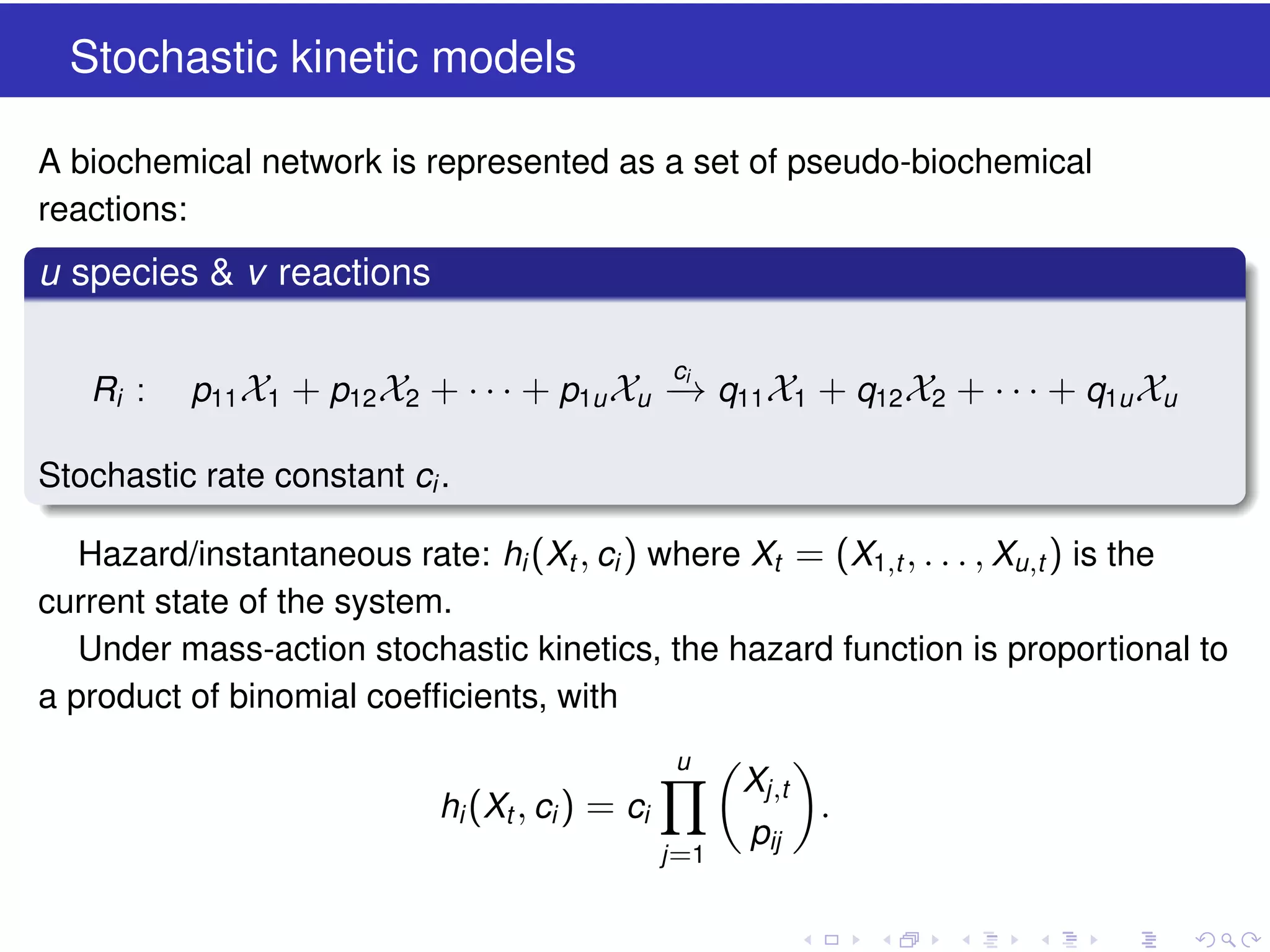
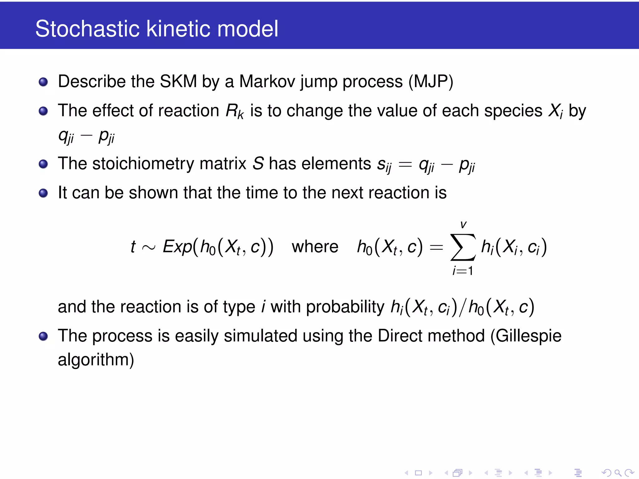
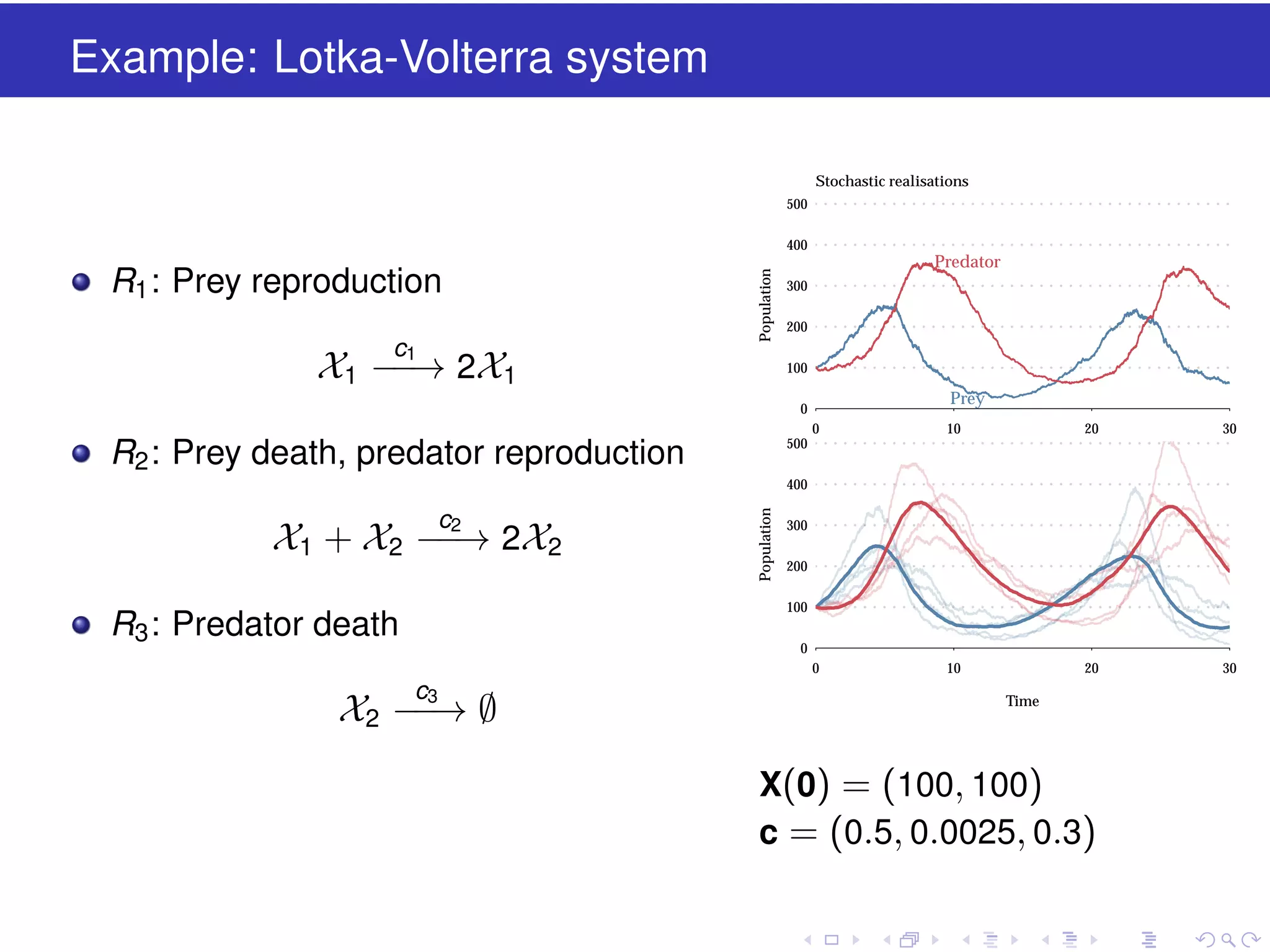
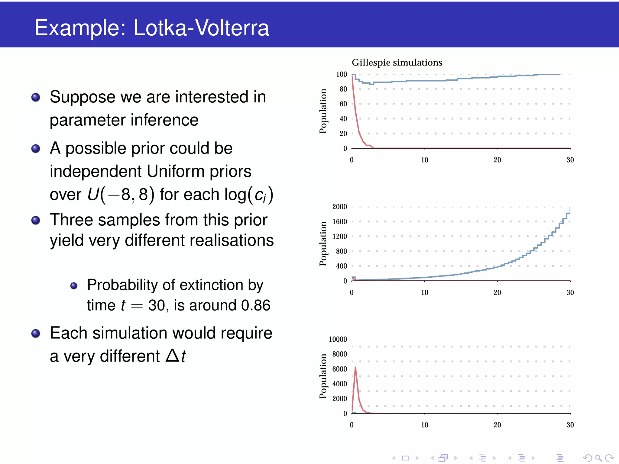
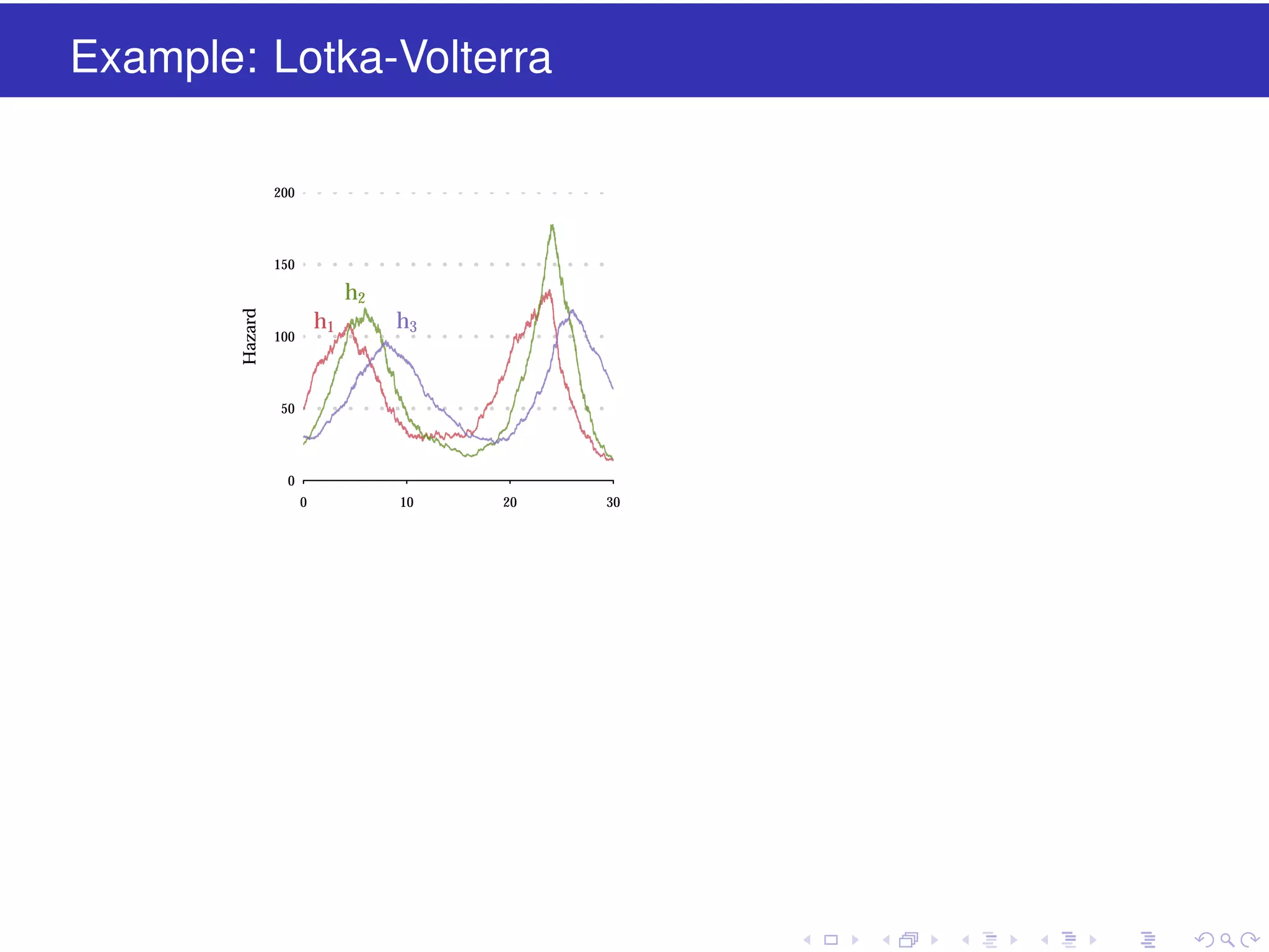
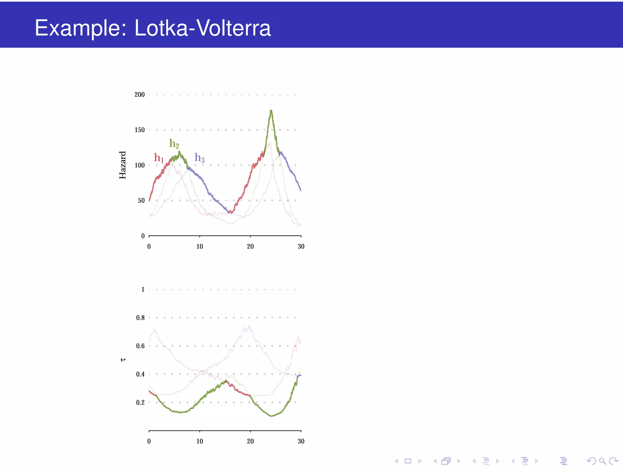
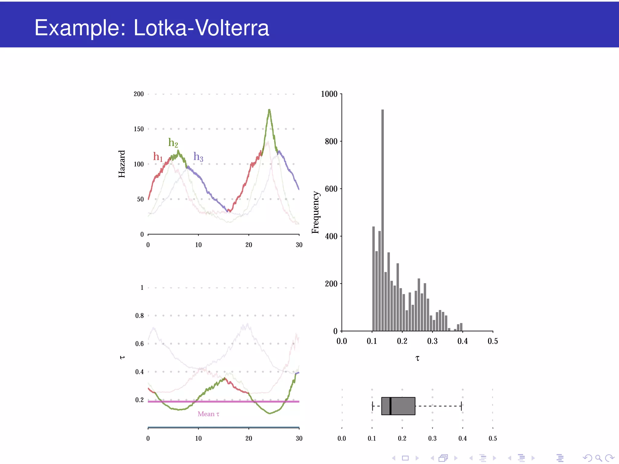
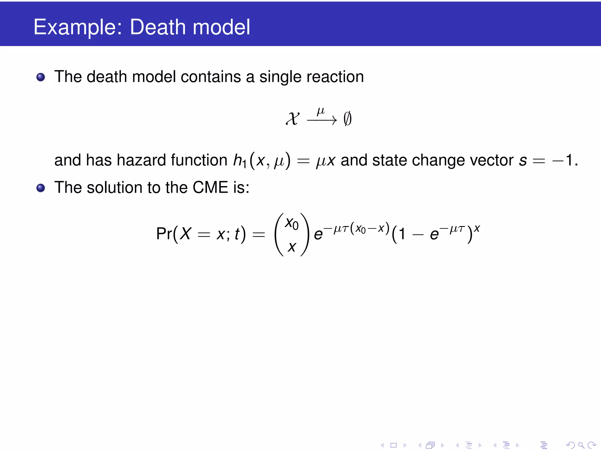
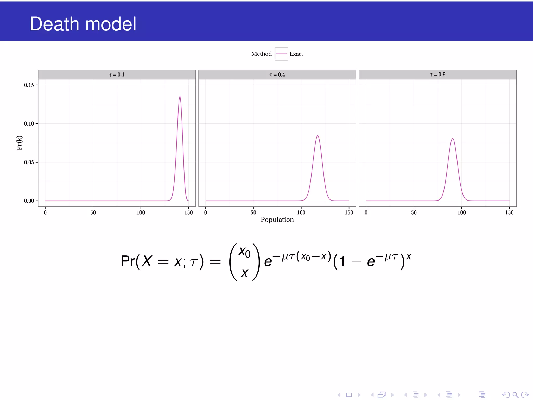
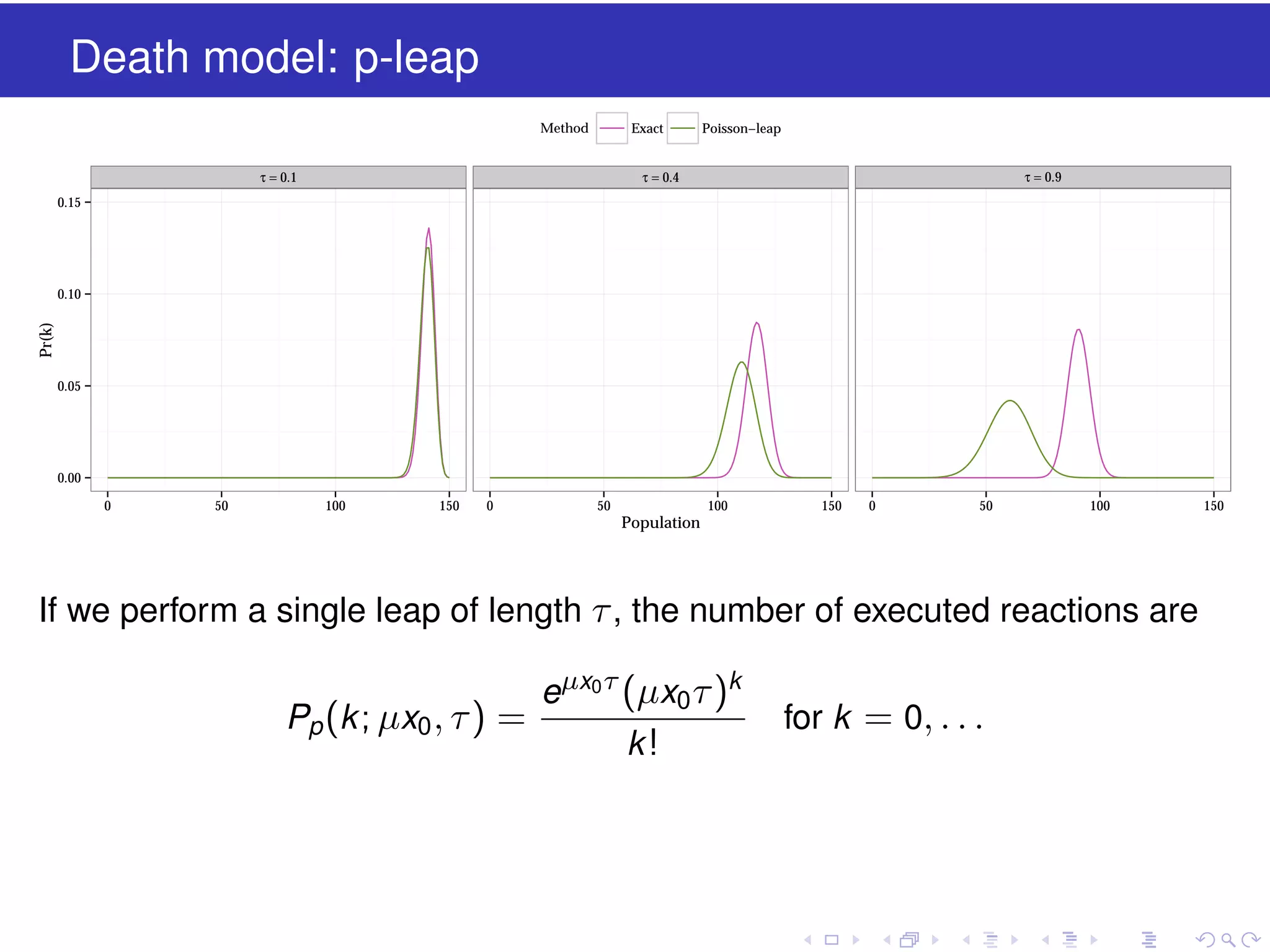
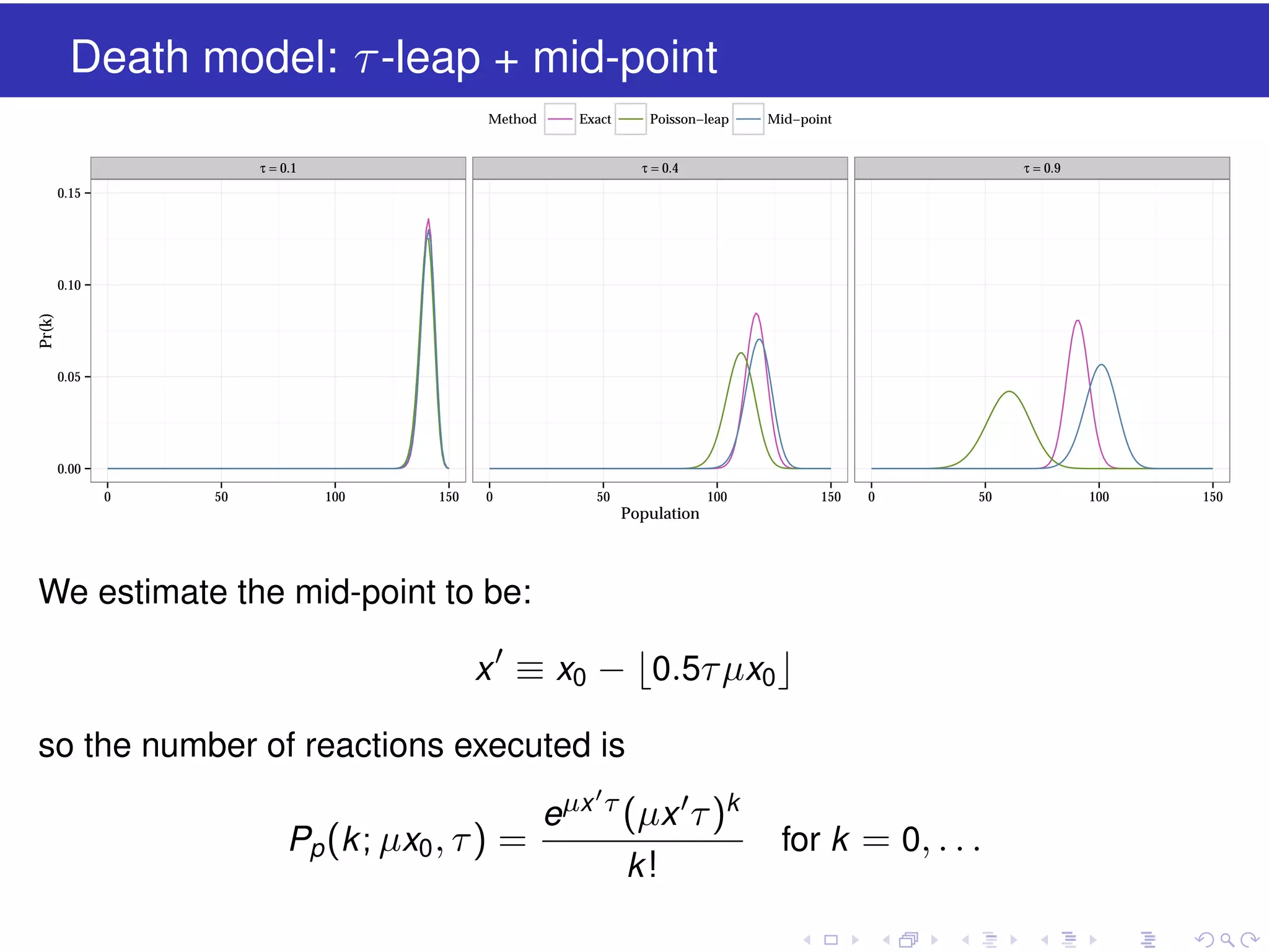
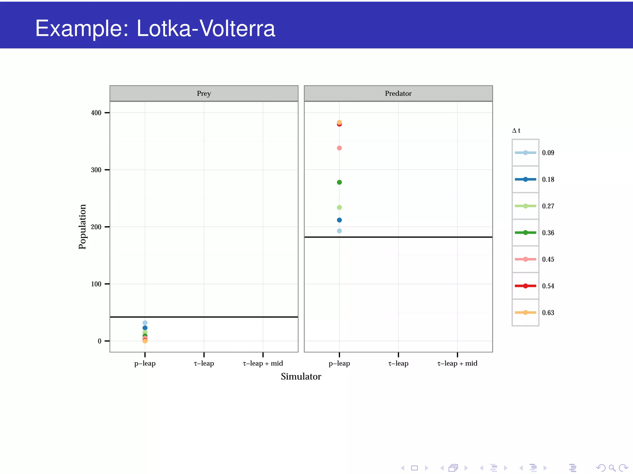
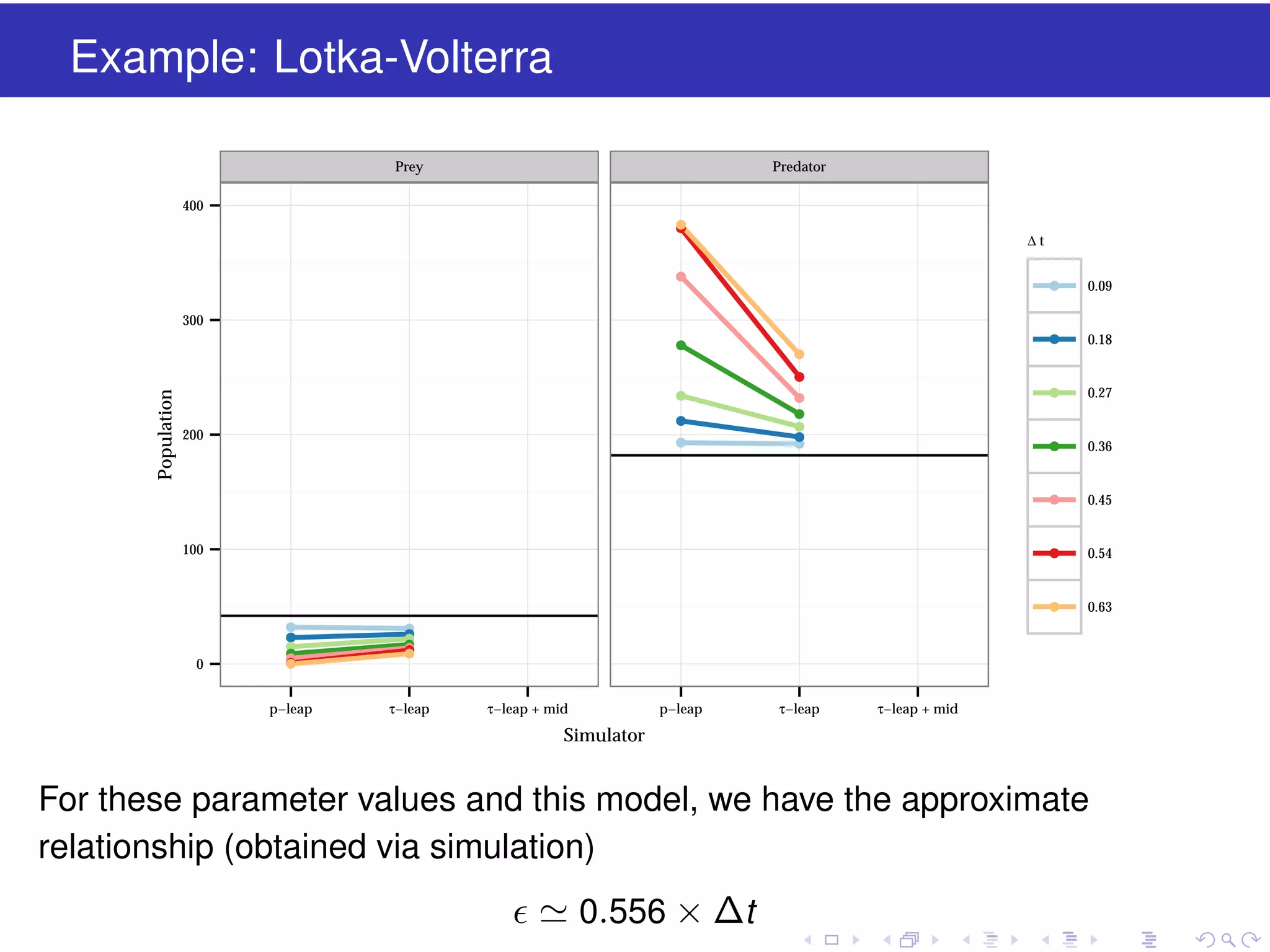
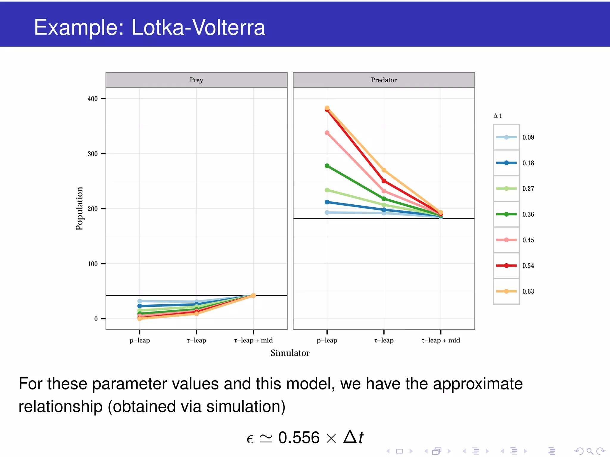
This document discusses approximate methods for simulating chemically reacting systems stochastically in a more computationally efficient manner than the direct method. It introduces the τ-leap method, where reactions are simulated in fixed time intervals (τ) by assuming reaction rates are constant over τ. It describes how τ can be chosen to satisfy a "leap condition" and minimize errors. The midpoint estimation technique is introduced to further reduce errors by estimating propensities at the midpoint of each τ interval. Examples applying these methods to a Lotka-Volterra system are provided to illustrate the techniques.

1. Approximate accelerated stochastic simulation of
chemically reacting systems
Colin Gillespie
October 16, 2013

2. Overview
Stochastic kinetic models
Issues with the Direct method
τ -leap method (Gillespie, 2001)
Leap conditions
Mid-point estimation
Examples
A
Source code (R and LTEX of these slides):
https://github.com/csgillespie/talks/

3. Stochastic kinetic models
A biochemical network is represented as a set of pseudo-biochemical
reactions:
u species & v reactions
Ri :
ci
p11 X1 + p12 X2 + · · · + p1u Xu − q11 X1 + q12 X2 + · · · + q1u Xu
→
Stochastic rate constant ci .
Hazard/instantaneous rate: hi (Xt , ci ) where Xt = (X1,t , . . . , Xu ,t ) is the
current state of the system.
Under mass-action stochastic kinetics, the hazard function is proportional to
a product of binomial coefficients, with
u
hi (Xt , ci ) = ci
j =1
Xj ,t
pij
.

4. Stochastic kinetic model
Describe the SKM by a Markov jump process (MJP)
The effect of reaction Rk is to change the value of each species Xi by
qji − pji
The stoichiometry matrix S has elements sij = qji − pji
It can be shown that the time to the next reaction is
v
t ∼ Exp(h0 (Xt , c )) where
h0 (Xt , c ) =
hi (Xi , ci )
i =1
and the reaction is of type i with probability hi (Xt , ci )/h0 (Xt , c )
The process is easily simulated using the Direct method (Gillespie
algorithm)

5. Example: Lotka-Volterra system
Stochastic realisations
500
c1
Population
400
R1 : Prey reproduction
X1 − → 2X1
−
Predator
300
200
100
Prey
0
0
10
0
20
10
30
20
30
500
R2 : Prey death, predator reproduction
X1 + X2 − → 2X2
−
Population
400
c2
300
200
100
R3 : Predator death
0
c3
X2 − → ∅
−
Time
X(0) = (100, 100)
c = (0.5, 0.0025, 0.3)

6. The direct method
1
Initialisation: initial conditions, reactions constants, and random number
generators
2
Propensities update: Update each of the v hazard functions, hi (x )
3
Propensities total: Calculate the total hazard h0 =
4
Reaction time: τ = −ln[U (0, 1)]/h0 and t = t + τ
5
Reaction selection: A reaction is chosen proportional to it’s hazard
6
Reaction execution: Update species
7
Iteration: If the simulation time is exceeded stop, otherwise go back to
step 2
Typically there are a large number of iterates
v
i =1
hi (x )

7. The direct method
1
Initialisation: initial conditions, reactions constants, and random number
generators
2
Propensities update: Update each of the v hazard functions, hi (x )
3
Propensities total: Calculate the total hazard h0 =
4
Reaction time: τ = −ln[U (0, 1)]/h0 and t = t + τ
5
Reaction selection: A reaction is chosen proportional to it’s hazard
6
Reaction execution: Update species
7
Iteration: If the simulation time is exceeded stop, otherwise go back to
step 2
Typically there are a large number of iterates
v
i =1
hi (x )

8. The direct method
1
Initialisation: initial conditions, reactions constants, and random number
generators
2
Propensities update: Update each of the v hazard functions, hi (x )
3
Propensities total: Calculate the total hazard h0 =
4
Reaction time: τ = −ln[U (0, 1)]/h0 and t = t + τ
5
Reaction selection: A reaction is chosen proportional to it’s hazard
6
Reaction execution: Update species
7
Iteration: If the simulation time is exceeded stop, otherwise go back to
step 2
Typically there are a large number of iterates
v
i =1
hi (x )

9. The direct method
1
Initialisation: initial conditions, reactions constants, and random number
generators
2
Propensities update: Update each of the v hazard functions, hi (x )
3
Propensities total: Calculate the total hazard h0 =
4
Reaction time: τ = −ln[U (0, 1)]/h0 and t = t + τ
5
Reaction selection: A reaction is chosen proportional to it’s hazard
6
Reaction execution: Update species
7
Iteration: If the simulation time is exceeded stop, otherwise go back to
step 2
Typically there are a large number of iterates
v
i =1
hi (x )

10. Approximations
Relax some assumptions (e.g. discreteness and stochasticity) in order to
make simulation faster and more scalable
Diffusion approximation / chemical Langevin equation (CLE)
Linear noise approximation (LNA) / moment closure (2MA)
ODE
Hybrid discrete-continuous models

11. Poisson leap
If all reactions are zeroth-order, then the model is a homogeneous
Poisson process
Hence the number of reactions in (t0 , t1 ) follows a Poisson distribution
For a more general model, if we consider a small time interval,
(t , t + ∆t ), then:
the hazard rates should be approximately constant
the number of reactions (of a given type) can be sampled from a Poisson
distribution
A balance between speed and accuracy

12. Poisson leap method
1
Set t = 0. Initialise the rate constants and the initial molecule numbers x
2
Calculate hi (x , ci ), for i = 1, . . . , v , and simulate the v -dimensional
reaction vector r , with i th entry a Po(hi (x , ci )∆t ) random quantity
3
Update the state according
4
Update t := t + ∆t
5
Output t and x. If t < Tmax return to step 2

13. Poisson leap method
1
Set t = 0. Initialise the rate constants and the initial molecule numbers x
2
Calculate hi (x , ci ), for i = 1, . . . , v , and simulate the v -dimensional
reaction vector r , with i th entry a Po(hi (x , ci )∆t ) random quantity
3
Update the state according
4
Update t := t + ∆t
5
Output t and x. If t < Tmax return to step 2
How do you chose ∆t?

14. Example: Lotka-Volterra
Gillespie simulations
100
80
Population
Suppose we are interested in
parameter inference
60
40
20
A possible prior could be
independent Uniform priors
over U (−8, 8) for each log(ci )
0
20
30
0
10
20
30
0
10
20
30
1600
1200
800
400
0
Probability of extinction by
time t = 30, is around 0.86
10000
Population
Each simulation would require
a very different ∆t
10
2000
Population
Three samples from this prior
yield very different realisations
0
8000
6000
4000
2000
0

15. Basic τ -leap method
Suppose a temporal leap τ will result in a state change λ
Choose a value of τ that satisfies the leap condition. For each reaction,
Rj , we want
|hj (x + λ) − hj (x)|
to be small
Sample kj ∼ P (hj (x)τ )
Compute λ
Set t := t + τ and x := x + λ

16. Choosing τ
If the reactions don’t depend on x, the leap condition will be satisfied
exactly for any τ (and so exact)
If population numbers are large, then it would take a large number of
reactions to “noticeably” change the hazard functions
If satisfying the leap condition requires a very small value τ << 1/h0 (x),
then we may as well use the exact SSA

17. A procedure for selecting τ (Gillespie 2001)
The expected net change in (t , t + τ ) will be:
v
¯
λ=
[hj (x)τ ]sj = τ ξ(x)
j =1
So we require that the expected changes in the propensity functions in
time τ , are bounded by some fraction of all propensity functions, i.e.
|hj (x + λ) − hj (x)| < h0 (x) for j = 1, . . . , v .
Estimate the difference using a Taylor expansion:
u
hj (x + λ) − hj (x)
τ ξi (x)
i =1
∂
hj (x)
∂ xi
Defining
bji (x) ≡
∂ hj (x)
∂ xi
(j = 1, . . . , v ; i = 1, . . . , u )

18. A procedure for selecting τ
The requirement becomes
u
ξi (x)bji (x) ≤ h0 (x) (j = 1, . . . , v )
τ
i =1
The largest value of τ consistent with this condition (and hence optimal) is
τ = min
j ∈[1,v ]
Typical values of
are around 0.05
h0 ( x)
u
i =1 ξi (x)bji (x)

19. Example: Lotka-Volterra
200
150
Hazard
h2
h1
100
h3
50
0
0
10
20
30

20. Example: Lotka-Volterra
200
150
Hazard
h2
h1
100
h3
50
0
0
10
20
30
0
10
20
30
1
0.8
τ
0.6
0.4
0.2

21. Example: Lotka-Volterra
200
150
Hazard
h2
h1
100
h3
50
0
0
10
20
30
0
10
20
30
1
0.8
τ
0.6
0.4
0.2

22. Example: Lotka-Volterra
1000
200
150
800
h3
Frequency
Hazard
h2
h1
100
50
0
0
10
20
600
400
30
200
1
0.8
0
0.0
0.6
0.1
0.2
0.3
0.4
0.5
0.3
0.4
0.5
τ
τ
0.4
0.2
Mean τ
0
10
20
30
0.0
0.1
0.2

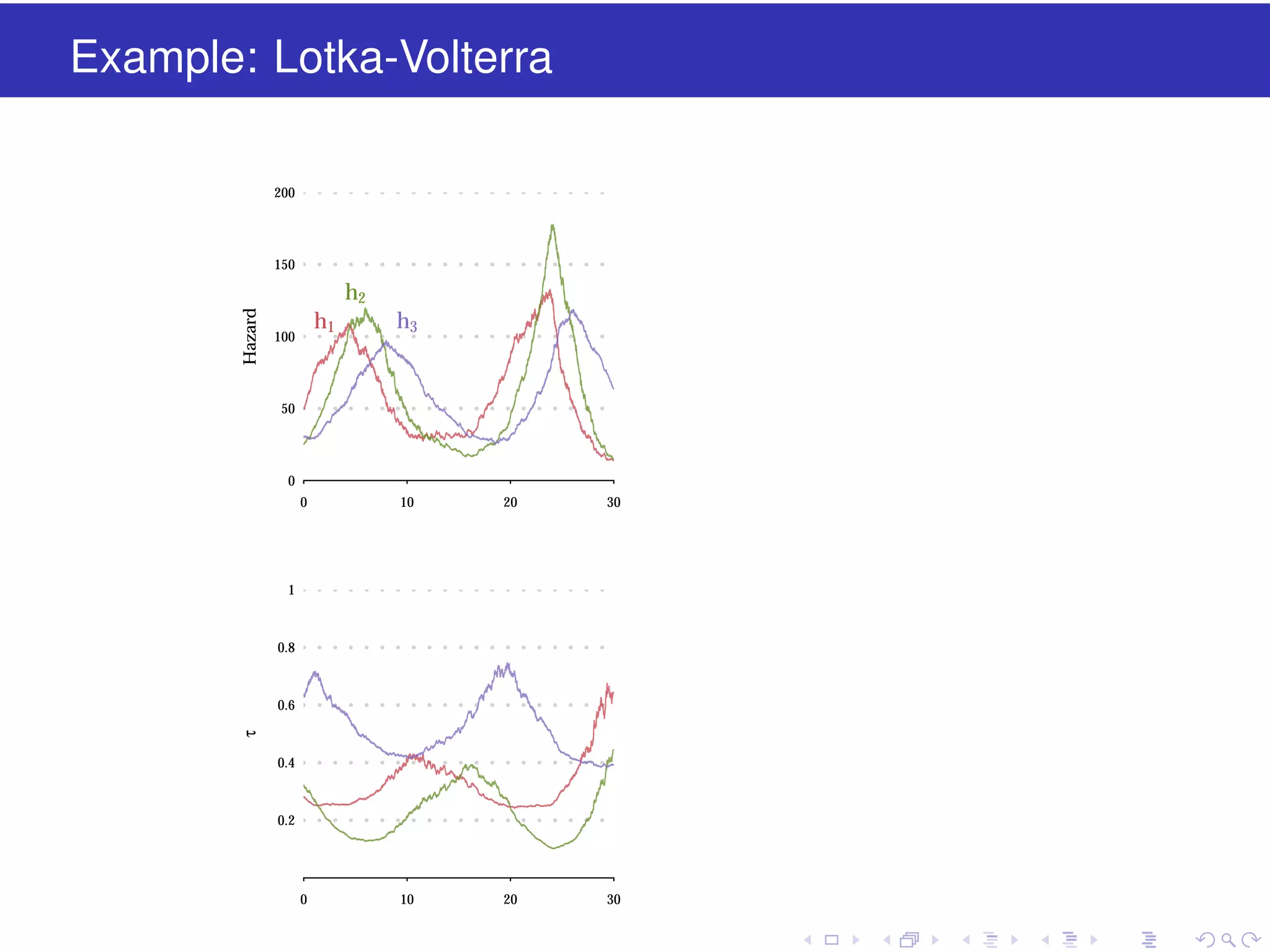
23. The estimated-midpoint technique
The leap condition requires that the hazards functions do not
“appreciably” change in the course of a leap
But we want to take large leaps, so we will inevitably get computational
errors
This is similar to solving the ODE
dX (t )
dt
= f (X )
using an Euler scheme
A standard technique is to use a second-order Runge-Kutta or modified
Euler method
X (t + ∆t ) = X (t ) + f [X (t ) + 0.5f (X (t ))∆t ]∆t
i.e. we use an Euler method to estimate the midpoint during [t , t + ∆t ],
then calculate the increment in X by evaluating the slope function f at that
estimated midpoint

24. Example: Death model
The death model contains a single reaction
µ
X −→ ∅
−
and has hazard function h1 (x , µ) = µx and state change vector s = −1.
The solution to the CME is:
Pr(X = x ; t ) =
x0
x
e−µτ (x0 −x ) (1 − e−µτ )x

25. Death model
Method
τ = 0.1
Exact
τ = 0.9
τ = 0.4
0.15
Pr(k)
0.10
0.05
0.00
0
50
100
150
0
50
100
150
0
Population
Pr(X = x ; τ ) =
x0
x
e−µτ (x0 −x ) (1 − e−µτ )x
50
100
150

26. Death model: p-leap
Method
Exact
τ = 0.1
Poisson−leap
τ = 0.9
τ = 0.4
0.15
Pr(k)
0.10
0.05
0.00
0
50
100
150
0
50
100
150
0
50
100
Population
If we perform a single leap of length τ , the number of executed reactions are
Pp (k ; µx0 , τ ) =
eµx0 τ (µx0 τ )k
k!
for k = 0, . . .
150

27. Death model: τ -leap + mid-point
Method
Exact
Poisson−leap
τ = 0.1
Mid−point
τ = 0.9
τ = 0.4
0.15
Pr(k)
0.10
0.05
0.00
0
50
100
150
0
50
100
150
0
50
Population
We estimate the mid-point to be:
x ≡ x0 − 0.5τ µx0
so the number of reactions executed is
Pp (k ; µx0 , τ ) =
eµx τ (µx τ )k
k!
for k = 0, . . .
100
150

28. Example: Lotka-Volterra
Prey
Predator
400
q
q
∆t
q
q
0.09
q
q
0.18
q
q
0.27
q
0.36
q
0.45
q
0.54
q
0.63
Population
300
q
200
q
100
0
q
q
q
q
q
q
p−leap
τ−leap
τ−leap + mid
Simulator
p−leap
τ−leap
τ−leap + mid

29. Example: Lotka-Volterra
Prey
Predator
400
q
q
∆t
q
q
0.09
q
0.18
q
0.27
q
0.36
q
0.45
q
0.54
q
0.63
300
q
q
Population
q
q
q
200
q
q
q
q
q
q
100
q
q
q
q
q
q
p−leap
0
q
q
q
q
q
q
τ−leap
τ−leap + mid
p−leap
τ−leap
τ−leap + mid
Simulator
For these parameter values and this model, we have the approximate
relationship (obtained via simulation)
0.556 × ∆t

30. Example: Lotka-Volterra
Prey
Predator
400
q
q
∆t
q
q
0.09
q
0.18
q
0.27
q
0.36
q
0.45
q
0.54
q
0.63
300
q
q
Population
q
q
q
200
q
q
q
q
q
q
q
q
q
100
q
q
q
q
q
q
p−leap
0
q
q
q
q
q
q
τ−leap
q
τ−leap + mid
p−leap
τ−leap
τ−leap + mid
Simulator
For these parameter values and this model, we have the approximate
relationship (obtained via simulation)
0.556 × ∆t

31. Summary
Similar issues arise when solving SDEs with the Euler-Maruyama
scheme
In fact, if we substitute Poisson with Gaussian random numbers in the
p-leap scheme, we get the Euler-Maruyama algorithm
Choosing a fixed ∆t for a wide range of parameter combinations doesn’t
make sense
Is it possible to these ideas when constructing bridges for SDEs?

32. References
Gillespie DT. Exact stochastic simulation of coupled chemical reactions. The
Journal of Physical Chemistry, 1977, 81: 2340 – 2361. Direct method
Gillespie, DT. Approximate accelerated stochastic simulation of chemically
reacting systems. The Journal of Chemical Physics, 2001, 115: 1716. τ -leap
method
Sandmann, W. Streamlined formulation of adaptive explicit-implicit tau-leaping
with automatic tau selection. Simulation Conference (WSC), Proceedings of the
2009 Winter. IEEE, 2009. Nice overview of the various τ -leap flavours.
Golightly, A & Gillespie, CS. Simulation of Stochastic Kinetic Models. In Silico
Systems Biology. Humana Press, 2013, 169 – 187. Overview of various SSA.
https://github.com/csgillespie/In-silico-Systems-Biology