This document is Mengdi Zheng's dissertation for the degree of Doctor of Philosophy in Applied Mathematics from Brown University. The dissertation focuses on developing numerical methods for stochastic partial differential equations (SPDEs) driven by Lévy jump processes. Chapter 1 introduces the motivation and challenges in uncertainty quantification of nonlinear SPDEs driven by Lévy noise. The subsequent chapters develop simulation methods for Lévy jump processes, adaptive stochastic collocation methods, and Wick-Malliavin approximations to solve SPDEs with discrete and tempered stable Lévy noise in multiple dimensions.


![List of Tables
4.1 For gPC with different orders P and WM with a fixed order of P =
3, Q = 2 in reaction equation (4.23) with one Poisson RV (λ = 0.5,
y0 = 1, k(ξ) = c0(ξ;λ)
2!
+ c1(ξ;λ)
3!
+ c2(ξ;λ)
4!
, σ = 0.1, RK4 scheme with
time step dt = 1e − 4), we compare: (1) computational complexity
ratio to evaluate k(t, ξ)y(t; ω) between gPC and WM (upper); (2) CPU
time ratio to compute k(t, ξ)y(t; ω) between gPC and WM (lower).We
simulated in Matlab on Intel (R) Core (TM) i5-3470 CPU @ 3.20 GHz. 69
4.2 Computational complexity ratio to evaluate u∂u
∂x
term in Burgers equa-
tion with d RVs between WM and gPC, as C(P,Q)d
(P+1)3d : here we take the
WM order as Q = P − 1, and gPC with order P, in different dimen-
sions d = 2, 3, and 50. . . . . . . . . . . . . . . . . . . . . . . . . . . . 83
5.1 MC/CP vs. MC/S: error l2u2(T) of the solution for Equation (5.1)
versus the number of samples s with λ = 10 (upper) and λ = 1
(lower). T = 1, c = 0.1, α = 0.5, = 0.1, µ = 2 (upper and lower).
Spatial discretization: Nx = 500 Fourier collocation points on [0, 2];
temporal discretization: first-order Euler scheme in (5.22) with time
steps t = 1 × 10⁻⁵
. In the CP approximation: RelTol = 1 × 10⁻⁸
for integration in U(δ). . . . . . . . . . . . . . . . . . . . . . . . . . . 102
xi](https://image.slidesharecdn.com/thesis-150401122906-conversion-gate01/85/Thesis-11-320.jpg)
![List of Figures
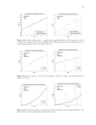
2.1 Empirical CDF of KL Expansion RVs Y1, ..., YM with M = 10 KL
expansion terms, for a centered Poisson process (Nt − λt) of λ =
10, Tmax = 1, with s = 10000 samples, and N = 200 points on the
time domain [0, 1]. . . . . . . . . . . . . . . . . . . . . . . . . . . . . 13
2.2 Exact sample path vs. sample path approximated by the KL ex-
pansion: when λ is smaller, the sample path is better approximated.
(Brownian motion is the limiting case for a centered poisson process
with very large birth rate.) . . . . . . . . . . . . . . . . . . . . . . . . 14
2.3 Exact mean vs. mean by KL expansion: when λ is larger, the KL
representation seems to be better. . . . . . . . . . . . . . . . . . . . . 14
2.4 Exact 2nd moment vs. 2nd moment by KL expansion with sampled
coefficients. The 2nd moments are not as well approximated as the
mean. . . . . . . . . . . . . . . . . . . . . . . . . . . . . . . . . . . . 14
3.1 Orthogonality defined in (3.27) with respect to the polynomial order
i up to 20 with Binomial distributions. . . . . . . . . . . . . . . . . . 32
3.2 CPU time to evaluate orthogonality for Binomial distributions. . . . . 33
3.3 Minimum polynomial order i (vertical axis) such that orth(i) is greater
than a threshold value. . . . . . . . . . . . . . . . . . . . . . . . . . . 34
3.4 Left: GENZ1 functions with different values of c and w; Right: h-
convergence of ME-PCM for function GENZ1. Two Gauss quadrature
points, d = 2, are employed in each element corresponding to a degree
m = 3 of exactness. c = 0.1, w = 1, ξ ∼ Bino(120, 1/2). Lanczos
method is employed to compute the orthogonal polynomials. . . . . . 42
3.5 Left: GENZ4 functions with different values of c and w; Right: h-
convergence of ME-PCM for function GENZ4. Two Gauss quadrature
points, d = 2, are employed in each element corresponding to a degree
m = 3 of exactness. c = 0.1, w = 1, ξ ∼ Bino(120, 1/2). Lanczos
method is employed for numerical orthogonality. . . . . . . . . . . . . 43
3.6 Non-nested sparse grid points with respect to sparseness parameter
k = 3, 4, 5, 6 for random variables ξ1, ξ2 ∼ Bino(10, 1/2), where the
one-dimensional quadrature formula is based on Gauss quadrature rule. 44
3.7 Convergence of sparse grids and tensor product grids to approximate
E[fi(ξ1, ξ2)], where ξ1 and ξ2 are two i.i.d. random variables associated
with a distribution Bino(10, 1/2). Left: f1 is GENZ1 Right: f4 is
GENZ4. Orthogonal polynomials are generated by Lanczos method. . 45
xii](https://image.slidesharecdn.com/thesis-150401122906-conversion-gate01/85/Thesis-12-320.jpg)
![3.8 Convergence of sparse grids and tensor product grids to approximate
E[fi(ξ1, ξ2, ..., ξ8)], where ξ1,...,ξ8 are eight i.i.d. random variables asso-
ciated with a distribution Bino(10, 1/2). Left: f1 is GENZ1 Right: f4
is GENZ4. Orthogonal polynomials are generated by Lanczos method. 45
3.9 p-convergence of PCM with respect to errors defined in equations
(3.54) and (3.55) for the reaction equation with t = 1, y0 = 1. ξ is
associated with negative binomial distribution with c = 1
2
and β = 1.
Orthogonal polynomials are generated by the Stieltjes method. . . . . 47
3.10 Left: exact solution of the KdV equation (3.65) at time t = 0, 1.
Right: the pointwise error for the soliton at time t = 1 . . . . . . . . 49
3.11 p-convergence of PCM with respect to errors defined in equations
(3.67) and (3.68) for the KdV equation with t = 1. a = 1, x0 = −5
and σ = 0.2, with 200 Fourier collocation points on the spatial domain
[−30, 30]. Left: ξ ∼Pois(10); Right: ξ ∼ Bino(n = 5, p = 1/2)). aPC
stands for arbitrary Polynomial Chaos, which is Polynomial Chaos
with respect to arbitrary measure. Orthogonal polynomials are gen-
erated by Fischer’s method. . . . . . . . . . . . . . . . . . . . . . . . 50
3.12 h-convergence of ME-PCM with respect to errors defined in equations
(3.67) and (3.68) for the KdV equation with t = 1.05, a = 1, x0 = −5,
σ = 0.2, and ξ ∼ Bino(n = 120, p = 1/2), with 200 Fourier collocation
points on the spatial domain [−30, 30], where two collocation points
are employed in each element. Orthogonal polynomials are generated
by the Fischer method (left) and the Stieltjes method (right). . . . . 51
3.13 Adapted mesh with five elements with respect to Pois(40) distribution. 52
3.14 p-convergence of ME-PCM on a uniform mesh and an adapted mesh
with respect to errors defined in equations (3.67) and (3.68) for the
KdV equation with t = 1, a = 1, x0 = −5, σ = 0.2, and ξ ∼
Pois(40), with 200 Fourier collocation points on the spatial domain
[−30, 30]. Left: Errors of the mean. Right: Errors of the second
moment. Orthogonal polynomials are generated by the Nowak method. 53
3.15 ξ1, ξ2 ∼ Bino(10, 1/2): convergence of sparse grids and tensor product
grids with respect to errors defined in equations (3.67) and (3.68) for
problem (3.69), where t = 1, a = 1, x0 = −5, and σ1 = σ2 = 0.2,
with 200 Fourier collocation points on the spatial domain [−30, 30].
Orthogonal polynomials are generated by the Lanczos method. . . . 54
3.16 ξ1 ∼ Bino(10, 1/2) and ξ2 ∼ N(0, 1): convergence of sparse grids and
tensor product grids with respect to errors defined in in equations
(3.67) and (3.68) for problem (3.69), where t = 1, a = 1, x0 = −5,
and σ1 = σ2 = 0.2, with 200 Fourier collocation points on the spatial
domain [−30, 30]. Orthogonal polynomials are generated by Lanczos
method. . . . . . . . . . . . . . . . . . . . . . . . . . . . . . . . . . . 55
3.17 Convergence of sparse grids and tensor product grids with respect to
errors defined in in equations (3.67) and (3.68) for problem (3.70),
where t = 0.5, a = 0.5, x0 = −5, σi = 0.1 and ξi ∼ Bino(5, 1/2), i =
1, 2, ..., 8, with 300 Fourier collocation points on the spatial domain
[−50, 50]. Orthogonal polynomials are generated by Lanczos method. 56
xiii](https://image.slidesharecdn.com/thesis-150401122906-conversion-gate01/85/Thesis-13-320.jpg)
![4.1 Reaction equation with one Poisson RV ξ ∼ Pois(λ) (d = 1): errors
versus final time T defined in (4.34) for different WM order Q in
equation (4.27), with polynomial order P = 10, y0 = 1, λ = 0.5. We
used RK4 scheme with time step dt = 1e − 4; k(ξ) = c0(ξ;λ)
2!
+ c1(ξ;λ)
3!
+
c2(ξ;λ)
4!
, σ = 0.1(left); k(ξ) = c0(ξ;λ)
0!
+ c1(ξ;λ)
3!
+ c2(ξ;λ)
6!
, σ = 1 (right). . . 68
4.2 Reaction equation with five Poisson RVs ξ1,...,5 ∼Pois(λ) (d = 5):
error defined in (4.34) with respect to time, for different WM order
Q, with parameters: λ = 1, σ = 0.5, y0 = 1, polynomial order P =
4, RK2 scheme with time step dt = 1e − 3, and k(ξ1, ξ2, ..., ξ5, t) =
5
i=1 cos(it)c1(ξi) in equation (4.23). . . . . . . . . . . . . . . . . . . 70
4.3 Reaction equation with one Poisson RV ξ1 ∼Pois(λ) and one Binomial
RV ξ2 ∼ Bino(N, p) (d = 2): error defined in (4.34) with respect to
time, for different WM order Q, with parameters: λ = 1, σ = 0.1,
N = 10, p = 1/2, y0 = 1, polynomial order P = 10, RK4 scheme with
time step dt = 1e − 4, and k(ξ1, ξ2, t) = c1(ξ1)k1(ξ2) in equation (4.23). 71
4.4 Burgers equation with one Poisson RV ξ ∼Pois(λ) (d = 1, ψ1(x, t) =
1): l2u2(T) error defined in (6.62) versus time, with respect to dif-
ferent WM order Q. Here we take in equation (4.32): polynomial
expansion order P = 6, λ = 1, ν = 1/2, σ = 0.1, IMEX (Crank-
Nicolson/RK2) scheme with time step dt = 2e − 4, and 100 Fourier
collocation points on [−π, π]. . . . . . . . . . . . . . . . . . . . . . . 73
4.5 P-convergence for Burgers equation with one Poisson RV ξ ∼Pois(λ)
(d = 1, ψ1(x, t) = 1): errors defined in equation (6.62) versus poly-
nomial expansion order P, for different WM order Q, and by prob-
abilistic collocation method (PCM) with P + 1 points with the fol-
lowing parameters: ν = 1, λ = 1, final time T = 0.5, IMEX (Crank-
Nicolson/RK2) scheme with time step dt = 5e − 4, 100 Fourier collo-
cation points on [−π, π], σ = 0.5 (left), and σ = 1 (right). . . . . . . 73
4.6 Q-convergence for Burgers equation with one Poisson RV ξ ∼Pois(λ)
(d = 1, ψ1(x, t) = 1): errors defined in equation (6.62) versus WM
order Q, for different polynomial order P, with the following param-
eters: ν = 1, λ = 1, final time T = 0.5, IMEX(RK2/Crank-Nicolson)
scheme with time step dt = 5e − 4, 100 Fourier collocation points on
[−π, π], σ = 0.5 (left), and σ = 1 (right). The dashed lines serve as a
reference of the convergence rate. . . . . . . . . . . . . . . . . . . . . 74
4.7 Burgers equation with three Poisson RVs ξ1,2,3 ∼Pois(λ) (d = 3): error
defined in equation (6.62) with respect to time, for different WM order
Q, with parameters: λ = 0.1, σ = 0.1, y0 = 1, ν = 1/100, polynomial
order P = 2, IMEX (RK2/Crank-Nicolson) scheme with time step
dt = 2.5e − 4. . . . . . . . . . . . . . . . . . . . . . . . . . . . . . . . 76
4.8 Reaction equation with P-adaptivity and two Poisson RVs ξ1,2 ∼Pois(λ)
(d = 2): error defined in (4.34) with two Poisson RVs by comput-
ing the WM propagator in equation (4.27) with respect to time by
the RK2 method with: fixed WM order Q = 1, y0 = 1, ξ1,2 ∼
Pois(1), a(ξ1, ξ2, t) = c1(ξ1; λ)c1(ξ2; λ), for fixed polynomial order
P (dashed lines), for varied polynomial order P (solid lines), for
σ = 0.1 (left), and σ = 1 (right). Adaptive criterion values are:
l2err(t) ≤ 1e − 8(left), and l2err(t) ≤ 1e − 6(right). . . . . . . . . . . 77
xiv](https://image.slidesharecdn.com/thesis-150401122906-conversion-gate01/85/Thesis-14-320.jpg)
![4.9 Burgers equation with P-Q-adaptivity and one Poisson RV ξ ∼Pois(λ)
(d = 1, ψ1(x, t) = 1): error defined in equation (6.62) by comput-
ing the WM propagator in equation (4.32) with IMEX (RK2/Crank-
Nicolson) method (λ = 1, ν = 1/2, time step dt = 2e − 4). Fixed
polynomial order P = 6, σ = 1, and Q is varied (left); fixed WM
order Q = 3, σ = 0.1, and P is varied (right). Adaptive criterion
value is: l2u2(T) ≤ 1e − 10 (left and right). . . . . . . . . . . . . . . 78
4.10 Terms in Q
p=0
P
i=0 ˆui
∂ˆuk+2p−i
∂x
Ki,k+2p−i,p for each PDE in the WM
propagator for Burgers equation with one RV in equation (4.38) are
denoted by dots on the grids: here P = 4, Q = 1
2
, k = 0, 1, 2, 3, 4. Each
grid represents a PDE in the WM propagator, labeled by k. Each dot
represents a term in the sum Q
p=0
P
i=0 ˆui
∂ˆuk+2p−i
∂x
Ki,k+2p−i,p . The
small index next to the dot is for p, x direction is the index i for ˆui,
and y direction is the index k + 2p − i in
∂ˆuk+2p−i
∂x
. The dots on the
same diagonal line have the same index p. . . . . . . . . . . . . . . . 81
4.11 The total number of terms as ˆum1...md
∂
∂x
ˆuk1+2p1−m1,...,kd+2pd−md
Km1,k1+2p1−m1,p1
...Kmd,kd+2pd−md,pd
in the WM propagator for Burgers equation with d
RVs, as C(P, Q)d
: for dimensions d = 2 (left) and d = 3 (right). Here
we assume P1 = ... = Pd = P and Q1 = ... = Qd = Q. . . . . . . . . . 83
5.1 Empirical histograms of an IG subordinator (α = 1/2) simulated via
the CP approximationat t = 0.5: the IG subordinator has c = 1,
λ = 3; each simulation contains s = 106
samples (we zoom in and plot
x ∈ [0, 1.8] to examine the smaller jumps approximation); they are
with different jump truncation sizes as δ = 0.1 (left, dotted, CPU time
1450s), δ = 0.02 (middle, dotted, CPU time 5710s), and δ = 0.005
(right, dotted, CPU time 38531s). The reference PDFs are plotted in
red solid lines; the one-sample K-S test values are calculated for each
plot; the RelTol of integration in U(δ) and bδ
is 1 × 10⁻⁸
. These runs
were done on Intel (R) Core (TM) i5-3470 CPU @ 3.20 GHz in Matlab. 99
5.2 Empirical histograms of an IG subordinator (α = 1/2) simulated via
the series representationat t = 0.5: the IG subordinator has c = 1,
λ = 3; each simulation is done on the time domain [0, 0.5] and con-
tains s = 106
samples (we zoom in and plot x ∈ [0, 1.8] to examine
the smaller jumps approximation); they are with different number of
truncations in the series as Qs = 10 (left, dotted, CPU time 129s),
Qs = 100 (middle, dotted, CPU time 338s), and Qs = 1000 (right,
dotted, CPU time 2574s). The reference PDFs are plotted in red
solid lines; the one-sample K-S test values are calculated for each
plot. These runs were done on Intel (R) Core (TM) i5-3470 CPU @
3.20 GHz in Matlab. . . . . . . . . . . . . . . . . . . . . . . . . . . . 99
5.3 PCM/CP vs. PCM/S: error l2u2(T) of the solution for Equation (5.1)
versus the number of jumps Qcp (in PCM/CP) or Qs (in PCM/S)
with λ = 10 (left) and λ = 1 (right). T = 1, c = 0.1, α = 0.5,
= 0.1, µ = 2, Nx = 500 Fourier collocation points on [0, 2] (left
and right). In the PCM/CP: RelTol = 1 × 10⁻¹⁰
for integration
in U(δ). In the PCM/S: RelTol = 1 × 10⁻⁸
for the integration of
E[((
αΓj
2cT
)−1/α
∧ ηjξ
1/α
j )2
]. . . . . . . . . . . . . . . . . . . . . . . . . . 107
xv](https://image.slidesharecdn.com/thesis-150401122906-conversion-gate01/85/Thesis-15-320.jpg)
![5.4 PCM vs. MC: error l2u2(T) of the solution for Equation (5.1) versus
the number of samples s obtained by MC/CP and PCM/CP with
δ = 0.01 (left) and MC/S with Qs = 10 and PCM/S (right). T = 1
, c = 0.1, α = 0.5, λ = 1, = 0.1, µ = 2 (left and right). Spatial
discretization: Nx = 500 Fourier collocation points on [0, 2] (left and
right); temporal discretization: first-order Euler scheme in (5.22) with
time steps t = 1 × 10⁻⁵
(left and right). In both MC/CP and
PCM/CP: RelTol = 1 × 10⁻⁸
for integration in U(δ). . . . . . . . . 109
5.5 Zoomed in density Pts(t, x) plots for the solution of Equation (5.2)
at different times obtained from solving Equation (5.37) for α = 0.5
(left) and Equation (5.42) for α = 1.5 (right): σ = 0.4, x0 = 1, c = 1,
λ = 10 (left); σ = 0.1, x0 = 1, c = 0.01, λ = 0.01 (right). We have
Nx = 2000 equidistant spatial points on [−12, 12] (left); Nx = 2000
points on [−20, 20] (right). Time step is t = 1 × 10⁻⁴
(left) and
t = 1 × 10⁻⁵
(right). The initial conditions are approximated by δD
20
(left and right). . . . . . . . . . . . . . . . . . . . . . . . . . . . . . 114
5.6 Density/CP vs. PCM/CP with the same δ: errors err1st and err2nd
of the solution for Equation (5.2) versus time obtained by the density
Equation (5.36) with CP approximation and PCM/CP in Equation
(5.55). c = 0.5, α = 0.95, λ = 10, σ = 0.01, x0 = 1 (left); c = 0.01,
α = 1.6, λ = 0.1, σ = 0.02, x0 = 1 (right). In the density/CP: RK2
with time steps t = 2 × 10⁻³
, 1000 Fourier collocation points on
[−12, 12] in space, δ = 0.012, RelTol = 1 × 10⁻⁸
for U(δ), and initial
condition as δD
20 (left and right). In the PCM/CP: the same δ = 0.012
as in the density/CP. . . . . . . . . . . . . . . . . . . . . . . . . . . 116
5.7 TFPDE vs. PCM/CP: error err2nd of the solution for Equation (5.2)
versus time with λ = 10 (left) and λ = 1 (right). Problems we are
solving: α = 0.5, c = 2, σ = 0.1, x0 = 1 (left and right). For
PCM/CP: RelTol = 1 × 10⁻⁸
for U(δ) (left and right). For the TF-
PDE: finite difference scheme in (5.47) with t = 2.5 × 10⁻⁵
, Nx
equidistant points on [−12, 12], initial condition given by δD
40 (left and
right). . . . . . . . . . . . . . . . . . . . . . . . . . . . . . . . . . . . 118
5.8 Zoomed in plots for the density Pts(x, T) by solving the TFPDE (5.37)
and the empirical histogram by MC/CP at T = 0.5 (left) and T = 1
(right): α = 0.5, c = 1, λ = 1, x0 = 1 and σ = 0.01 (left and
right). In the MC/CP: sample size s = 105
, 316 bins, δ = 0.01,
RelTol = 1 × 10⁻⁸
for U(δ), time step t = 1 × 10⁻³
(left and
right). In the TFPDE: finite difference scheme given in (5.47) with
t = 1 × 10⁻⁵
in time, Nx = 2000 equidistant points on [−12, 12]
in space, and the initial conditions are approximated by δD
40 (left and
right). We perform the one-sample K-S tests here to test how two
methods match. . . . . . . . . . . . . . . . . . . . . . . . . . . . . . 119
6.1 An illustration of the applications of multi-dimensional L´evy jump
models in mathematical finance. . . . . . . . . . . . . . . . . . . . . 127
6.2 Three ways to correlate L´evy pure jump processes. . . . . . . . . . . 128
6.3 The L´evy measures of bivariate tempered stable Clayton processes
with different dependence strength (described by the correlation length
τ) between their L1 and L2 components. . . . . . . . . . . . . . . . . 133
xvi](https://image.slidesharecdn.com/thesis-150401122906-conversion-gate01/85/Thesis-16-320.jpg)
![6.4 The L´evy measures of bivariate tempered stable Clayton processes
with different dependence strength (described by the correlation length
τ) between their L++
1 and L++
2 components (only in the ++ corner).
It shows how the dependence structure changes with respect to the
parameter τ in the Clayton family of copulas. . . . . . . . . . . . . . 134
6.5 trajectory of component L++
1 (t) (in blue) and L++
2 (t) (in green) that
are dependent described by Clayton copula with dependent structure
parameter τ. Observe how trajectories get more similar when τ in-
creases. . . . . . . . . . . . . . . . . . . . . . . . . . . . . . . . . . . . 137
6.6 Sample path of (L1, L2) with marginal L´evy measure given by equation
(6.14), L´evy copula given by (6.13), with each components such as
F++
given by Clayton copula with parameter τ. Observe that when τ
is bigger, the ’flipping’ motion happens more symmetrically, because
there is equal chance for jumps to be the same sign with the same
size, and for jumps to be the opposite signs with the same size. . . . 139
6.7 Sample paths of bivariate tempered stable Clayton L´evy jump pro-
cesses (L1, L2) simulated by the series representation given in Equa-
tion (6.30). We simulate two sample paths for each value of τ. . . . . 140
6.8 An illustration of the three methods used in this paper to solve the
moment statistics of Equation (6.1). . . . . . . . . . . . . . . . . . . 140
6.9 An illustration of the three methods used in this paper to solve the
moment statistics of Equation (6.1). . . . . . . . . . . . . . . . . . . 147
6.10 An illustration of the three methods used in this paper to solve the
moment statistics of Equation (6.1). . . . . . . . . . . . . . . . . . . 148
6.11 PCM/S (probabilistic) vs. MC/S (probabilistic): error l2u2(t) of the
solution for Equation (6.1) with a bivariate pure jump L´evy process
with the L´evy measure in radial decomposition given by Equation
(6.9) versus the number of samples s obtained by MC/S and PCM/S
(left) and versus the number of collocation points per RV obtained
by PCM/S with a fixed number of truncations Q in Equation (6.10)
(right). t = 1 , c = 1, α = 0.5, λ = 5, µ = 0.01, NSR = 16.0%
(left and right). In MC/S: first order Euler scheme with time step
t = 1 × 10⁻³
(right). . . . . . . . . . . . . . . . . . . . . . . . . . . 151
6.12 PCM/series rep v.s. exact: T = 1. We test the noise/signal=variance/mean
ratio to be 4% at T = 1. . . . . . . . . . . . . . . . . . . . . . . . . . 152
6.13 PCM/series d-convergence and Q-convergence at T=1. We test the
noise/signal=variance/mean ratio to be 4% at t=1. The l2u2 error is
defined as l2u2(t) =
||Eex[u2(x,t;ω)]−Enum[u2(x,t;ω)]||L2([0,2])
||Eex[u2(x,t;ω)]||L2([0,2])
. . . . . . . . . . 153
6.14 MC v.s. exact: T = 1. Choice of parameters of this problem: we
evaluated the moment statistics numerically with integration rela-
tive tolerance to be 10−8
. With this set of parameter, we test the
noise/signal=variance/mean ratio to be 4% at T = 1. . . . . . . . . . 153
6.15 MC v.s. exact: T = 2. Choice of parameters of this problem: we
evaluated the moment statistics numerically with integration rela-
tive tolerance to be 10−8
. With this set of parameter, we test the
noise/signal=variance/mean ratio to be 10% at T = 2. . . . . . . . . 154
xvii](https://image.slidesharecdn.com/thesis-150401122906-conversion-gate01/85/Thesis-17-320.jpg)

![6.23 S-convergence in MC/S with 10-dimensional L´evy jump processes:difference
in the E[u2
] (left) between different sample sizes s and s = 106
(as a
reference). The heat equation (6.1) is driven by a 10-dimensional jump
process with a L´evy measure (6.9) obtained by MC/S with series rep-
resentation (6.10). We show the L2 norm of these differences versus
s (right). Final time T = 1, c = 0.1, α = 0.5, λ = 10, µ = 0.01, time
step t = 4 × 10⁻³
, and Q = 10. The NSR at T = 1 is 6.62%. . . . . 167
6.24 Samples of (u1, u2) (left) and joint PDF of (u1, u2, ..., u10) on the
(u1, u2) plane by MC (right) : c = 0.1, α = 0.5, λ = 10, µ = 0.01,dt =
4e − 3 (first order Euler scheme), T = 1, Q = 10 (number of trunca-
tions in the series representation), and sample size s = 106
. . . . . . 167
6.25 Samples of (u9, u10) (left) and joint PDF of (u1, u2, ..., u10) on the
(u9, u10) plane by MC (right) : c = 0.1, α = 0.5, λ = 10, µ = 0.01,dt =
4e − 3 (first order Euler scheme), T = 1, Q = 10 (number of trunca-
tions in the series representation), and sample size s = 106
. . . . . . . 168
6.26 First two moments for solution of the heat equation (6.1) driven by a
10-dimensional jump process with a L´evy measure (6.9) obtained by
MC/S with series representation (6.10) at final time T = 0.5 (left) and
T = 1 (right) by MC : c = 0.1, α = 0.5, λ = 10, µ = 0.01, dt = 4e − 3
(with the first order Euler scheme), Q = 10, and sample size s = 106
. 169
6.27 Q-convergence in PCM/S with 10-dimensional L´evy jump processes:difference
in the E[u2
] (left) between different series truncation order Q and
Q = 16 (as a reference). The heat equation (6.1) is driven by a
10-dimensional jump process with a L´evy measure (6.9) obtained by
MC/S with series representation (6.10). We show the L2 norm of these
differences versus Q (right). Final time T = 1, c = 0.1, α = 0.5, λ =
10, µ = 0.01. The NSR at T = 1 is 6.62%. . . . . . . . . . . . . . . . 169
6.28 MC/S V.s. PCM/S with 10-dimensional L´evy jump processes:difference
between the E[u2
] computed from MC/S and that computed from
PCM/S at final time T = 0.5 (left) and T = 1 (right). The heat equa-
tion (6.1) is driven by a 10-dimensional jump process with a L´evy
measure (6.9) obtained by MC/S with series representation (6.10).
c = 0.1, α = 0.5, λ = 10, µ = 0.01. In MC/S, time step t = 4×10⁻³
,
Q = 10. In PCM/S, Q = 16. . . . . . . . . . . . . . . . . . . . . . . . 170
6.29 The function in Equation (6.82) with d = 2 (left up and left down)
and the ANOVA approximation of it with effective dimension of two
(right up and right down). A = 0.5, d = 2. . . . . . . . . . . . . . . . 173
6.30 The function in Equation (6.82) with d = 2 (left up and left down)
and the ANOVA approximation of it with effective dimension of two
(right up and right down). A = 0.1, d = 2. . . . . . . . . . . . . . . . 173
6.31 The function in Equation (6.82) with d = 2 (left up and left down)
and the ANOVA approximation of it with effective dimension of two
(right up and right down). A = 0.01, d = 2. . . . . . . . . . . . . . . 174
xix](https://image.slidesharecdn.com/thesis-150401122906-conversion-gate01/85/Thesis-19-320.jpg)
![6.32 1D-ANOVA-FP V.s. 2D-ANOVA-FP with 10-dimensional L´evy jump processes:the
mean (left) for the solution of the heat equation (6.1) driven by a 10-
dimensional jump process with a L´evy measure (6.9) computed by
1D-ANOVA-FP, 2D-ANOVA-FP, and PCM/S. The L2 norms of dif-
ference in E[u] between these three methods are plotted versus final
time T (right). c = 1, α = 0.5, λ = 10, µ = 10−4
. In 1D-ANOVA-FP:
t = 4 × 10⁻³
in RK2, M = 30 elements, q = 4 GLL points on
each element. In 2D-ANOVA-FP: t = 4 × 10⁻³
in RK2, M = 5
elements on each direction, q2
= 16 GLL points on each element. In
PCM/S: Q = 10 in the series representation (6.10). Initial condition
of ANOVA-FP: MC/S data at t0 = 0.5, s = 1 × 10⁴
, t = 4 × 10⁻³
.
NSR ≈ 18.24% at T = 1. . . . . . . . . . . . . . . . . . . . . . . . . 175
6.33 1D-ANOVA-FP V.s. 2D-ANOVA-FP with 10-dimensional L´evy jump processes:the
second moment (left) for the solution of heat equation (6.1) driven by
a 10-dimensional jump process with a L´evy measure (6.9) computed
by 1D-ANOVA-FP, 2D-ANOVA-FP, and PCM/S. The L2 norms of
difference in E[u2
] between these three methods are plotted versus
final time T (right). c = 1, α = 0.5, λ = 10, µ = 10−4
. In 1D-ANOVA-
FP: t = 4 × 10⁻³
in RK2, M = 30 elements, q = 4 GLL points
on each element. In 2D-ANOVA-FP: t = 4 × 10⁻³
in RK2, M = 5
elements on each direction, q2
= 16 GLL points on each element. Ini-
tial condition of ANOVA-FP: MC/S data at t0 = 0.5, s = 1 × 10⁴
,
t = 4×10⁻³
. In PCM/S: Q = 10 in the series representation (6.10).
NSR ≈ 18.24% at T = 1. . . . . . . . . . . . . . . . . . . . . . . . . 176
6.34 Evolution of marginal distributions pi(xi, t) at final time t = 0.6, ..., 1.
c = 1 , α = 0.5, λ = 10, µ = 10−4
. Initial condition from MC:
t0 = 0.5, s = 104
, dt = 4 × 10⁻³
, Q = 10. 1D-ANOVA-FP : RK2
with time step dt = 4 × 10⁻³
, 30 elements with 4 GLL points on each
element . . . . . . . . . . . . . . . . . . . . . . . . . . . . . . . . . . 177
6.35 Showing the mean E[u] at different final time by PCM (Q = 10) and
by solving 1D-ANOVA-FP equations. c = 1 , α = 0.5, λ = 10,
µ = 1e − 4. Initial condition from MC: s = 104
, dt = 4−3
, Q = 10.
1D-ANOVA-FP : RK2 with dt = 4 × 10⁻³
, 30 elements with 4 GLL
points on each element. . . . . . . . . . . . . . . . . . . . . . . . . . 178
6.36 The mean E[u2
] at different final time by PCM (Q = 10) and by
solving 1D-ANOVA-FP equations. c = 1 , α = 0.5, λ = 10, µ = 1e−4.
Initial condition from MC: s = 104
, dt = 4 × 10⁻³
, Q = 10. 1D-
ANOVA-FP : RK2 with dt = 4 × 10⁻³
, 30 elements with 4 GLL
points on each element. . . . . . . . . . . . . . . . . . . . . . . . . . 179
6.37 The mean E[u2
] at different final time by PCM (Q = 10) and by
solving 2D-ANOVA-FP equations. c = 1 , α = 0.5, λ = 10, µ = 10−4
.
Initial condition from MC: s = 104
, dt = 4 × 10⁻³
, Q = 10. 2D-
ANOVA-FP : RK2 with dt = 4 × 10⁻³
, 30 elements with 4 GLL
points on each element. . . . . . . . . . . . . . . . . . . . . . . . . . 180
6.38 Left: sensitivity index defined in Equation (6.87) on each pair of
(i, j), j ≥ i. Right: sensitivity index defined in Equation (6.88) on
each pair of (i, j), j ≥ i. They are computed from the MC data at
t0 = 0.5 with s = 104
samples. . . . . . . . . . . . . . . . . . . . . . 182
xx](https://image.slidesharecdn.com/thesis-150401122906-conversion-gate01/85/Thesis-20-320.jpg)
![6.39 Error growth by 2D-ANOVA-FP in different dimension d:the error growth
l2u1rel(T; t0) in E[u] defined in Equation (6.91) versus final time T
(left); the error growth l2u2rel(T; t0) in E[u2
] defined in Equation
(6.92) versus T (middle); l2u1rel(T = 1; t0) and l2u2rel(T = 1; t0)
versus dimension d (right). We consider the diffusion equation (6.1)
driven by a d-dimensional jump process with a L´evy measure (6.9)
computed by 2D-ANOVA-FP, and PCM/S. c = 1, α = 0.5, µ = 10−4
(left, middle, right). In Equation (6.49): t = 4 × 10⁻³
in RK2,
M = 30 elements, q = 4 GLL points on each element. In Equation
(6.50): t = 4 × 10⁻³
in RK2, M = 5 elements on each direction,
q2
= 16 GLL points on each element. Initial condition of ANOVA-FP:
MC/S data at t0 = 0.5, s = 1 × 10⁴
, t = 4 × 10⁻³
, and Q = 16. In
PCM/S: Q = 16 in the series representation (6.10). NSR ≈ 20.5%
at T = 1 for all the dimensions d = 2, 4, 6, 10, 14, 18. These runs were
done on Intel (R) Core (TM) i5-3470 CPU @ 3.20 GHz in Matlab. . . 184
7.1 Summary of thesis . . . . . . . . . . . . . . . . . . . . . . . . . . . . 189
xxi](https://image.slidesharecdn.com/thesis-150401122906-conversion-gate01/85/Thesis-21-320.jpg)

![2
1.1 Motivation
Stochastic partial differential equations (SPDEs) are widely used for stochastic mod-
eling in diverse applications from physics, to engineering, biology and many other
fields, where the source of uncertainty includes random coefficients and stochastic
forcing. Our work is motivated by two things: application and shortcomings of past
work.
The source of uncertainty, practically, can be any non-Gaussian process. In many
cases, the random parameters are only observed at discrete values, which implies
that a discrete probability measure is more appropriate from the modeling point of
view. More generally, random processes with jumps are of fundamental importance in
stochastic modeling, e.g., stochastic-volatility jump-diffusion models in finance [171],
stochastic simulation algorithms for modeling diffusion, reaction and taxis in biol-
ogy [41], fluid models with jumps [158], quantum-jump models in physics [35], etc.
This serves as the motivation of our work on simulating SPDEs driven by discrete
random variables (RVs). Nonlinear SPDEs with discrete RVs and jump processes are
of practical use, since sources of stochastic excitations including uncertain parame-
ters and boundary/initial conditions are typically observed at discrete values. Many
complex systems of fundamental and industrial importance are significantly affected
by the underlying fluctuations/variations in random excitations, such as stochastic-
volatility jump-diffusion model in mathematical finance [12, 13, 24, 27, 28, 171],
stochastic simulation algorithms for modeling diffusion, reaction and taxis in biol-
ogy [41], truncated Levy flight model in turbulence [85, 106, 121, 158], quantum-jump
models in physics [35], etc.
An interesting source of uncertainty is L´evy jump processes, such as tempered](https://image.slidesharecdn.com/thesis-150401122906-conversion-gate01/85/Thesis-23-320.jpg)
![3
α stable (TαS) processes. TαS processes were introduced in statistical physics to
model turbulence, e.g., the truncated L´evy flight model [85, 106, 121], and in math-
ematical finance to model stochastic volatility, e.g., the CGMY model [27, 28]. The
empirical distribution of asset prices is not always in a stable distribution or a nor-
mal distribution. The tail is heavier than a normal distribution and thinner than a
stable distribution [20]. Therefore, the TαS process was introduced as the CGMY
model to modify the Black and Scholes model. More details of white noise the-
ory for L´evy jump processes with applications to SPDEs and finance can be found
in [18, 120, 96, 97, 124]. Although one-dimensional (1D) jump models are constructed
in finance with L´evy processes [14, 86, 100], many financial models require multi-
dimensional L´evy jump processes with dependent components [33], such as basket
option pricing [94], portfolio optimization [39], and risk scenarios for portfolios [33].
In history, multi-dimensional Gaussian models are widely applied in finance because
of the simplicity in the description of dependence structures [134], however in some
applications we must take jumps in price processes into account [27, 28].
This work is constructed on previous work on the field of uncertainty quan-
tification (UQ), which includes the generalized polynomial chaos method (gPC),
multi-element generalized polynomial chaos method (MEgPC), probabilistic collo-
cation method (PCM), sparse collocation method, analysis of variance (ANOVA),
and many other variants (see, e.g., [8, 9, 50, 52, 58, 156] and references therein).
1.1.1 Computational limitations for UQ of nonlinear SPDEs
Numerically, nonlinear SPDEs with discrete processes are often solved by gPC in-
volving a system of coupled deterministic nonlinear equations [169], or probabilistic
collocation method (PCM) [50, 170, 177] involving nonlinear corresponding PDEs](https://image.slidesharecdn.com/thesis-150401122906-conversion-gate01/85/Thesis-24-320.jpg)
![4
obtained at the collocation points. For stochastic processes with short correlation
length, the number of RVs required to represent the processes can be extremely large.
Therefore, the number of equations involved in the gPC propagator for a nonlinear
SPDE driven by such a process can be very large and highly coupled.
1.1.2 Computational limitations for UQ of SPDEs driven by
L´evy jump processes
For simulations of L´evy jump processes as TαS, we do not know the distribution of in-
crements explicitly [33], but we may still simulate the trajectories of TαS processes by
the random walk approximation [10]. However, the random walk approximation does
not identify the jump time and size of the large jumps precisely [139, 140, 141, 142].
In the heavy tailed case, large jumps contribute more than small jumps in functionals
of a L´evy process. Therefore, in this case, we have mainly used two other ways to
simulate the trajectories of a TαS process numerically: compound Poisson (CP) ap-
proximation [33] and series representation [140]. In the CP approximation, we treat
the jumps smaller than a certain size δ by their expectation, and treat the remaining
process with larger jumps as a CP process [33]. There are six different series represen-
tations of L´evy jump processes. They are the inverse L´evy measure method [44, 82],
LePage’s method [92], Bondesson’s method [23], thinning method [140], rejection
method [139], and shot noise method [140, 141]. However, in each representation,
the number of RVs involved is very large (such as 100). In this work, for TαS pro-
cesses, we will use the shot noise representation for Lt as a series representation
method because the tail of L´evy measure of a TαS process does not have an explicit
inverse [142]. Both the CP and the series approximation converge slowly when the
jumps of the L´evy process are highly concentrated around zero, however both can](https://image.slidesharecdn.com/thesis-150401122906-conversion-gate01/85/Thesis-25-320.jpg)
![5
be improved by replacing the small jumps via Brownian motions [6]. The α-stable
distribution was introduced to model the empirical distribution of asset prices [104],
replacing the normal distribution. In the past literature, the simulation of SDEs or
functionals of TαS processes was mainly done via MC [128]. MC for functionals of
TαS processes is possible after a change of measure that transform TαS processes
into stable processes [130].
1.2 Introduction of TαS L´evy jump processes
TαS processes were introduced in statistical physics to model turbulence, e.g., the
truncated L´evy flight model [85, 106, 121], and in mathematical finance to model
stochastic volatility, e.g., the CGMY model [27, 28]. Here, we consider a symmet-
ric TαS process (Lt) as a pure jump L´evy martingale with characteristic triplet
(0, ν, 0) [19, 143] (no drift and no Gaussian part). The L´evy measure is given by [33]
1
:
ν(x) =
ce−λ|x|
|x|α+1
, 0 < α < 2. (1.1)
This L´evy measure can be interpreted as an Esscher transformation [57] from that
of a stable process with exponential tilting of the L´evy measure. The parameter
c > 0 alters the intensity of jumps of all given sizes; it changes the time scale of
the process. Also, λ > 0 fixes the decay rate of big jumps, while α determines the
relative importance of smaller jumps in the path of the process2
. The probability
density for Lt at a given time is not available in a closed form (except when α = 1
2
3
).
1
In a more generalized form, L´evy measure is ν(x) = c−e−λ−|x|
|x|α+1 Ix<0 + c+e−λ+|x|
|x|α+1 Ix>0. We may
have different coefficients c+, c−, λ+, λ− on the positive and the negative jump parts.
2
In the case when α = 0, Lt is the gamma process.
3
See inverse Gaussian processes.](https://image.slidesharecdn.com/thesis-150401122906-conversion-gate01/85/Thesis-26-320.jpg)
![6
The characteristic exponent for Lt is [33]:
Φ(s) = s−1
log E[eisLs
] = 2Γ(−α)λα
c[(1 −
is
λ
)α
− 1 +
isα
λ
], α = 1, (1.2)
where Γ(x) is the Gamma function and E is the expectation. By taking the deriva-
tives of the characteristic exponent we obtain the mean and variance:
E[Lt] = 0, V ar[Lt] = 2tΓ(2 − α)cλα−2
. (1.3)
In order to derive the second moments for the exact solutions of Equations (5.1) and
(5.2), we introduce the Itˆo isometry. The jump of Lt is defined by Lt = Lt − Lt− .
We define the Poisson random measure N(t, U) as [71, 119, 123]:
N(t, U) =
0≤s≤t
I Ls∈U , U ∈ B(R0), ¯U ⊂ R0. (1.4)
Here R0 = R{0}, and B(R0) is the σ-algebra generated by the family of all Borel
subsets U ⊂ R, such that ¯U ⊂ R0; IA is an indicator function. The Poisson random
measure N(t, U) counts the number of jumps of size Ls ∈ U at time t. In order
to introduce the Itˆo isometry, we define the compensated Poisson random measure
˜N [71] as:
˜N(dt, dz) = N(dt, dz) − ν(dz)dt = N(dt, dz) − E[N(dt, dz)]. (1.5)
The TαS process Lt (as a martingale) can be also written as:
Lt =
t
0 R0
z ˜N(dτ, dz). (1.6)
For any t, let Ft be the σ-algebra generated by (Lt, ˜N(ds, dz)), z ∈ R0, s ≤ t. We
define the filtration to be F = {Ft, t ≥ 0}. If a stochastic process θt(z), t ≥ 0, z ∈ R0](https://image.slidesharecdn.com/thesis-150401122906-conversion-gate01/85/Thesis-27-320.jpg)
![7
is Ft-adapted, we have the following Itˆo isometry [119]:
E[(
T
0 R0
θt(z) ˜N(dt, dz))2
] = E[
T
0 R0
θ2
t (z)ν(dz)dt]. (1.7)
1.3 Organization of the thesis
In Chapter 2, we discuss four methods to simulate L´evy jump processes preliminar-
ies and background information to the reader: 1. random walk approximation; 2.
Karhumen-Loeve expansion; 3. compound Poisson approximation; 4. series repre-
sentation.
In Chapter 3, The methods of generating orthogonal polynomial bases with re-
spect to discrete measures are presented, followed by a discussion about the error of
numerical integration. Numerical solutions of the stochastic reaction equation and
Korteweg- de Vries (KdV) equation, including adaptive procedures, are explained.
Then, we summarize the work. In the appendices, we provide more details about
the deterministic KdV equation solver, and the adaptive procedure.
In Chapter 4, we define the WM expansion and derive the Wick-Malliavin prop-
agators for a stochastic reaction equation and a stochastic Burgers equation. We
present several numerical results for SPDEs with one RV and multiple RVs, in-
cluding an adaptive procedure to control the error in time. We also compare the
computational complexity between gPC and WM for stochastic Burgers equation
with the same level of accuracy. Also, we provide an iterative algorithm to generate
coefficients in the WM approximation.
In Chapter 5, we compare the CP approximation and the series representation](https://image.slidesharecdn.com/thesis-150401122906-conversion-gate01/85/Thesis-28-320.jpg)


![10
In general there are three ways to generate a L´evy process [140]: random walk ap-
proximation, series representation and compound Poisson (CP) approximation. The
random walk approximation approximate the continuous random walk by a discrete
random walk on a discrete time sequence, if the marginal distribution of the process is
known. It is often used to simulate L´evy jump processes with large jumps, but it does
not identify the jump time and size of the large jumps precisely [139, 140, 141, 142].
We attempt to simulate a non-Gaussian process by Karhumen-Lo`eve (KL) expansion
here as well by computing the covariance kernel and its eigenfunctions. In the CP
approximation, we treat the jumps smaller than a certain size by their expectation
as a drift term, and the remaining process with large jumps as a CP process [33].
There are six different series representations of L´evy jump processes. They are the in-
verse L´evy measure method [44, 82], LePage’s method [92], Bondesson’s method [23],
thinning method [140], rejection method [139], and shot noise method [140, 141].
2.1 Random walk approximation to Poisson pro-
cesses
For a L´evy jump process Lt, on a fixed time grid [t0, t1, t2, ..., tN ], we may approximate
Lt by Lt = N
i=1 XiI{t < ti}. When the marginal distribution of Lt is known,
the distribution of Xi is known to be Lti−ti−1
. Therefore, on the fixed time grid,
we may generate the RVs Xi by sampling from the known distribution. When Lt
is composed of large jumps with low intensity (or rate of jumps), this can be a
good approximation. However, we are mostly interested in L´evy jump processes
with infinite activity (with high rates of jumps), therefore this will not be a good
approximation for the kind of processes we are going to consider, such as tempered](https://image.slidesharecdn.com/thesis-150401122906-conversion-gate01/85/Thesis-31-320.jpg)
![11
α stable processes.
2.2 KL expansion for Poisson processes
Let us first take a Poisson process N(t; ω) with intensity λ on a computational time
domain [0, T] as an example. We mimic the KL expansion for Gaussian processes to
simulate non-Gaussian processes as Poisson processes.
• First we calculate the covariance kernel (assuming t > t).
Cov(N(t; ω)N(t ; ω)) = E[N(t; ω)N(t ; ω)] − E[N(t; ω)]E[N(t ; ω)]
= E[N(t; ω)N(t; ω)] + E[N(t; ω)]E[N(t − t; ω)] − E[N(t; ω)]E[N(t ; ω)]
= λt, t > t,
(2.1)
Therefore, the covariance kernel is
Cov(N(t; ω)N(t ; ω)) = λ(t t ) (2.2)
• The eigenvalues and eigenfunctions for this kernel would be:
ek(t) =
√
2sin(k −
1
2
)πt (2.3)
and
λk =
1
(k − 1
2
)2π2
(2.4)
where k=1,2,3,...
• The stochastic process Nt approximated by finite number of terms in the KL](https://image.slidesharecdn.com/thesis-150401122906-conversion-gate01/85/Thesis-32-320.jpg)
![12
expansion can be written as:
˜N(t; ω) = λt +
M
i=1
λiYiei(t) (2.5)
where
1
0
e2
k(t)dt = 1 (2.6)
and
T
0
e2
k(t)dt = T −
sin[T(1 − 2k)π]
π(1 − 2k)
(2.7)
and they are orthogonal.
• The distribution of Yk can be calculated by the following. Given a sample path
ω ∈ Ω,
< N(t; ω) − λt, ek(t) >=
Yk
√
λ
π(k − 1
2
)
< ek(t), ek(t) >
= 2Yk
√
λ[
T(2k − 1)π − sin((2k − 1)πT)
π2(2k − 1)2
]
=< N(t; ω), ek(t) > −
√
2λ
π2
[−2πTcos(πT/2) + 4sin(πT/2)].
(2.8)
Therefore,
Yk =
π2
(2k − 1)2
[< N(t; ω), ek(t) > −
√
2λ
π2 [−2πTcos(πT/2) + 4sin(πT/2)]]
2
√
λ[T(2k − 1)π − sin((2k − 1)πT]
.
(2.9)
From each sample path each sample path ω, we can calculate the value of
Y1, ..., YM . In this way the distribution of Y1, ..., YM can be sampled. Nu-
merically, if we simulate enough number of samples of a Poisson process (by
simulating the jump times and jump sizes separately), we may have the em-
pirical distribution of RVs Y1, ..., YM .
• Now let us see how well the sample paths of the Poisson process Nt are ap-](https://image.slidesharecdn.com/thesis-150401122906-conversion-gate01/85/Thesis-33-320.jpg)
![13
5 4 3 2 1 0 1 2 3 4 5
0
0.1
0.2
0.3
0.4
0.5
0.6
0.7
0.8
0.9
1
Empirical CDF for KL Exp RVs
i
CDF
Figure 2.1: Empirical CDF of KL Expansion RVs Y1, ..., YM with M = 10 KL expansion terms,
for a centered Poisson process (Nt −λt) of λ = 10, Tmax = 1, with s = 10000 samples, and N = 200
points on the time domain [0, 1].
proximated by the KL expansion.
• Now let us see how well the mean of the Poisson process Nt are approximated
by the KL expansion.
• Now let us see how well the second moment of the Poisson process Nt are
approximated by the KL expansion.
2.3 Compound Poisson approximation to L´evy jump
processes
Let us take a tempered α stable process (TαS) as an example here. TαS processes
were introduced in statistical physics to model turbulence, e.g., the truncated L´evy
flight model [85, 106, 121], and in mathematical finance to model stochastic volatility,
e.g., the CGMY model [27, 28]. Here, we consider a symmetric TαS process (Lt) as
a pure jump L´evy martingale with characteristic triplet (0, ν, 0) [19, 143] (no drift](https://image.slidesharecdn.com/thesis-150401122906-conversion-gate01/85/Thesis-34-320.jpg)
![15
and no Gaussian part). The L´evy measure is given by [33] 1
:
ν(x) =
ce−λ|x|
|x|α+1
, 0 < α < 2. (2.10)
This L´evy measure can be interpreted as an Esscher transformation [57] from that
of a stable process with exponential tilting of the L´evy measure. The parameter
c > 0 alters the intensity of jumps of all given sizes; it changes the time scale of
the process. Also, λ > 0 fixes the decay rate of big jumps, while α determines the
relative importance of smaller jumps in the path of the process2
. The probability
density for Lt at a given time is not available in a closed form (except when α = 1
2
3
).
The characteristic exponent for Lt is [33]:
Φ(s) = s−1
log E[eisLs
] = 2Γ(−α)λα
c[(1 −
is
λ
)α
− 1 +
isα
λ
], α = 1, (2.11)
where Γ(x) is the Gamma function and E is the expectation. By taking the deriva-
tives of the characteristic exponent we obtain the mean and variance:
E[Lt] = 0, V ar[Lt] = 2tΓ(2 − α)cλα−2
. (2.12)
In the CP approximation, we simulate the jumps larger than δ as a CP process
and replace jumps smaller than δ by their expectation as a drift term [33]. Here
we explain the method to approximate a TαS subordinator Xt (without a Gaussian
part and a drift) with the L´evy measure ν(x) = ce−λx
xα+1 Ix>0 (positive jumps only); this
method can be generalized to a TαS process with both positive and negative jumps.
1
In a more generalized form, L´evy measure is ν(x) = c−e−λ−|x|
|x|α+1 Ix<0 + c+e−λ+|x|
|x|α+1 Ix>0. We may
have different coefficients c+, c−, λ+, λ− on the positive and the negative jump parts.
2
In the case when α = 0, Lt is the gamma process.
3
See inverse Gaussian processes.](https://image.slidesharecdn.com/thesis-150401122906-conversion-gate01/85/Thesis-36-320.jpg)
![16
The CP approximation Xδ
t for this TαS subordinator Xt is:
Xt ≈ Xδ
t =
s≤t
XsI Xs≥δ+E[
s≤t
XsI Xs<δ] =
∞
i=1
Jδ
i It≤Ti
+bδ
t ≈
Qcp
i=1
Jδ
i It≤Ti
+bδ
t,
(2.13)
We introduce Qcp here as the number of jumps occurred before time t. The first
term ∞
i=1 Jδ
i It≤Ti
is a compound Poisson process with jump intensity
U(δ) = c
∞
δ
e−λx
dx
xα+1
(2.14)
and jump size distribution pδ
(x) = 1
U(δ)
ce−λx
xα+1 Ix≥δ for Jδ
i . The jump size random
variables (RVs) Jδ
i are generated via the rejection method [37]. This is the algorithm
of rejection method to generate RVs with distribution pδ
(x) = 1
U(δ)
ceλx
xα+1 Ix≥δ for CP
approximation [37]
The distribution pδ
(x) can be bounded by
pδ
(x) ≤
δ−α
e−λδ
αU(δ)
fδ
(x), (2.15)
where fδ
(x) = αδ−α
xα+1 Ix≥δ. The algorithm to generate RVs with distribution pδ
(x) =
1
U(δ)
ceλx
xα+1 Ix≥δ is [33, 37]:
• REPEAT
• Generate RVs W and V : independent and uniformly distributed on [0, 1]
• Set X = δW−1/α](https://image.slidesharecdn.com/thesis-150401122906-conversion-gate01/85/Thesis-37-320.jpg)
![17
• Set T = fδ(X)δ−αe−λδ
pδ(X)αU(δ)
• UNTIL V T ≤ 1
• RETURN X .
Here, Ti is the i-th jump arrival time of a Poisson process with intensity U(δ).
The accuracy of CP approximation method can be improved by replacing the smaller
jumps by a Brownian motion [6], when the growth of the L´evy measure near zero
is fast. The second term functions as a drift term, bδ
t, resulted from truncating
the smaller jumps. The drift is bδ
= c
δ
0
e−λxdx
xα . This integration diverges when
α ≥ 1, therefore the CP approximation method only applies to TαS processes with
0 < α < 1. In this paper, both the intensity U(δ) and drift bδ
are calculated
via numerical integrations with Gauss-quadrature rules [54] with a specified relative
tolerance (RelTol) 4
. In general, there are two algorithms to simulate a compound
Poisson process [33]: the first method is to simulate the jump time Ti by exponentially
distributed RVs and take the number of jumps Qcp as large as possible; the second
method is to first generate and fix the number of jumps, then generate the jump time
by uniformly distributed RVs on [0, t]. Algorithms for simulating a CP process (the
second kind) with intensity and the jump size distribution in their explicit forms are
known on a fixed time grid [33]. Here we describe how to simulate the trajectories of a
CP process with intensity U(δ) and jump size distribution νδ(x)
U(δ)
, on a simulation time
domain [0, T] at time t. The algorithm to generate sample paths for CP processes
without a drift:
4
The RelTol of numerical integration is defined as |q−Q|
|Q| , where q is the computed value of the
integral and Q is the unknown exact value.](https://image.slidesharecdn.com/thesis-150401122906-conversion-gate01/85/Thesis-38-320.jpg)
![18
• Simulate an RV N from Poisson distribution with parameter U(δ)T, as the
total number of jumps on the interval [0, T].
• Simulate N independent RVs, Ti, uniformly distributed on the interval [0, T],
as jump times.
• Simulate N jump sizes, Yi with distribution νδ(x)
U(δ)
.
• Then the trajectory at time t is given by N
i=1 ITi≤tYi.
In order to simulate the sample paths of a symmetric TαS process with a L´evy
measure given in Equation (5.3), we generate two independent TαS subordinators
via the CP approximation and subtract one from the other. The accuracy of the CP
approximation is determined by the jump truncation size δ.
The numerical experiments for this method will be given in Chapter 5.
2.4 Series representation to L´evy jump processes
Let { j}, {ηj}, and {ξj} be sequences of i.i.d. RVs such that P( j = ±1) = 1/2, ηj ∼
Exponential(λ), and ξj ∼Uniform(0, 1). Let {Γj} be arrival times in a Poisson
process with rate one. Let {Uj} be i.i.d. uniform RVs on [0, T]. Then, a TαS
process Lt with L´evy measure given in Equation (5.3) can be represented as [142]:
Lt =
+∞
j=1
j[(
αΓj
2cT
)−1/α
∧ ηjξ
1/α
j ]I{Uj≤t}, 0 ≤ t ≤ T. (2.16)
Equation (5.14) converges almost surely as uniformly in t [139]. In numerical simu-
lations, we truncate the series in Equation (5.14) up to Qs terms. The accuracy of](https://image.slidesharecdn.com/thesis-150401122906-conversion-gate01/85/Thesis-39-320.jpg)


![22
3.2 Generation of orthogonal polynomials for dis-
crete measures
Let µ be a positive measure with infinite support S(µ) ⊂ R and finite moments at
all orders, i.e.,
S
ξn
µ(dξ) < ∞, ∀n ∈ N0, (3.1)
where N0 = {0, 1, 2, ...}, and it is defined as a Riemann-Stieltjes integral. There
exists one unique [54] set of orthogonal monic polynomials {Pi}∞
i=0 with respect to
the measure µ such that
S
Pi(ξ)Pj(ξ)µ(dξ) = δijγ−2
i , i = 0, 1, 2, . . . , (3.2)
where γi = 0 are constants. In particular, the orthogonal polynomials satisfy a
three-term recurrence relation [31, 43]
Pi+1(ξ) = (ξ − αi)Pi(ξ) − βiPi−1(ξ), i = 0, 1, 2, . . . (3.3)
The uniqueness of the set of orthogonal polynomials with respect to µ can be also
derived by constructing such set of polynomials starting from P0(ξ) = 1. We typ-
ically choose P−1(ξ) = 0 and β0 to be a constant. Then the full set of orthogonal
polynomials is completely determined by the coefficients αi and βi.
If the support S(µ) is a finite set with data points {τ1, ..., τN }, i.e., µ is a discrete
measure defined as
µ =
N
i=1
λiδτi
, λi > 0, (3.4)](https://image.slidesharecdn.com/thesis-150401122906-conversion-gate01/85/Thesis-43-320.jpg)
![23
the corresponding orthogonality condition is finite, up to order N − 1 [46, 54], i.e.,
S
P2
i (ξ)µ(dξ) = 0, i ≥ N, (3.5)
where δτi
indicates the empirical measure at τi, although by the recurrence relation
(3.3) we can generate polynomials at any order greater than N − 1. Furthermore,
one way to test whether the coefficients αi are well approximated is to check the
following relation [45, 46]
N−1
i=0
αi =
N
i=1
τi. (3.6)
One can prove that the coefficient of ξN−1
in PN (ξ) is − N−1
i=0 αi, and PN (ξ) =
(ξ − τ1)...(ξ − τN ), therefore equation (3.6) holds [46].
We subsequently examine five different approaches of generating orthogonal poly-
nomials for a discrete measure and point out the pros and cons of each method. In
Nowak method, the coefficients of the polynomials are directly derived from solving
a linear system; in the other four methods, we generate coefficients αi and βi by four
different numerical methods, and the coefficients of polynomials are derived from the
recurrence relation in equation (3.3).
3.2.1 Nowak method
Define the k-th order moment as
mk =
S
ξk
µ(dξ), k = 0, 1, ..., 2d − 1. (3.7)](https://image.slidesharecdn.com/thesis-150401122906-conversion-gate01/85/Thesis-44-320.jpg)
![24
The coefficients of the d-th order polynomial Pd(ξ) = d
i=0 aiξi
are determined by
the following linear system [125]
m0 m1 . . . md
m1 m2 . . . md+1
. . . . . . . . . . . .
md−1 md . . . m2d−1
0 0 . . . 1
a0
a1
. . .
ad−1
ad
=
0
0
. . .
0
1
, (3.8)
where the (d + 1) by (d + 1) Vandermonde matrix needs to be inverted.
Although this method is straightforward to implement, it is well known that the
matrix may be ill conditioned when d is very large.
The total computational complexity for solving the linear system in equation
(3.8) is O(d2
) to generate Pd(ξ) 1
.
3.2.2 Stieltjes method
Stieltjes method is based on the following formulas of the coefficients αi and βi [54]
αi = S
ξP2
i (ξ)µ(dξ)
S
P2
i (ξ)µ(dξ)
, βi = S
ξP2
i (ξ)µ(dξ)
S
P2
i−1(ξ)µ(dξ)
, i = 0, 1, .., d − 1. (3.9)
For a discrete measure, the Stieltjes method is quite stable [54, 51]. When the
discrete measure has a finite number of elements in its support (N), the above
formulas are exact. However, if we use Stieltjes method on a discrete measure with
infinite support, i.e. Poisson distribution, we approximate the measure by a discrete
1
Here we notice that the Vandermonde matrix is in a Toeplitz matrix form. Therefore the
computational complexity of solving this linear system is O(d2
) [59, 157].](https://image.slidesharecdn.com/thesis-150401122906-conversion-gate01/85/Thesis-45-320.jpg)
![25
measure with finite number of points; therefore, each time when we iterate for αi
and βi, the error accumulates by neglecting the points with less weights. In that
case, αi and βi may suffer from inaccuracy when i is close to N [54].
The computational complexity for integral evaluation in equation (3.9) is of the
order O(N).
3.2.3 Fischer method
Fischer proposed a procedure for generating the coefficients αi and βi by adding
data points one-by-one [45, 46]. Assume that the coefficients αi and βi are known
for the discrete measure µ = N
i=1 λiδτi
. Then, if we add another data point τ to
the discrete measure µ and define a new discrete measure ν = µ + λδτ , λ being the
weight of the newly added data point τ, the following relations hold [45, 46]:
αν
i = αi + λ
γ2
i Pi(τ)Pi+1(τ)
1 + λ i
j=0 γ2
j P2
j (τ)
− λ
γ2
i−1Pi(τ)Pi−1(τ)
1 + λ i−1
j=0 γ2
j P2
j (τ)
(3.10)
βν
i = βi
[1 + λ i−2
j=0 γ2
j P2
j (τ)][1 + λ i
j=0 γ2
j P2
j (τ)]
[1 + λ i−1
j=0 γ2
j P2
j (τ)]2
(3.11)
for i < N, and
αν
N = τ − λ
γ2
N−1PN (τ)PN−1(τ)
1 + λ N−1
j=0 γ2
j P2
j (τ)
(3.12)
βν
N =
λγ2
N−1P2
N (τ)[1 + λ N−2
j=0 γ2
j P2
j (τ)]
[1 + λ N−1
j=0 γ2
j P2
j (τ)]2
, (3.13)
where αν
i and βν
i indicate the coefficients in the three-term recurrence formula (3.3)
for the measure ν. The numerical stability of this algorithm depends on the stability
of the recurrence relations above, and on the sequence of data points added [46]. For](https://image.slidesharecdn.com/thesis-150401122906-conversion-gate01/85/Thesis-46-320.jpg)
![26
example, the data points can be in either ascending or descending order. Fischer’s
method basically modifies the available coefficients αi and βi using the information
induced by the new data point. Thus, this approach is very practical when an
empirical distribution for stochastic inputs is altered by an additional possible value.
For example, let us consider that we have already generated d probability collocation
points with respect to the given discrete measure with N data points, and we want
to add another data point into the discrete measure to generate d new probability
collocation points with respect to the new measure. Using the Nowak method, we
will need to reconstruct the moment matrix and invert the matrix again with N + 1
data points; however by Fischer’s method, we will only need to update 2d values of
αi and βi by adding this new data point, which is more convenient.
We generate a new sequence of {αi, βi} by adding a new data point into the
measure, therefore the computational complexity for calculating the coefficients
{γ2
i , i = 0, .., d} for N times is O(N2
).
3.2.4 Modified Chebyshev method
Compared to the Chebyshev method [54], the modified Chebyshev method computes
moments in a different way. Define the quantities:
µi,j =
S
Pi(ξ)ξj
µ(dξ), i, j = 0, 1, 2, ... (3.14)
Then, the coefficients αi and βi satisfy [54]:
α0 =
µ0,1
µ0,0
, β0 = µ0,0, αi =
µi,i+1
µi,i
−
µi−1,i
µi−1,i−1
, βi =
µi,i
µi−1,i−1
. (3.15)](https://image.slidesharecdn.com/thesis-150401122906-conversion-gate01/85/Thesis-47-320.jpg)
![27
Note that due to the orthogonality, µi,j = 0 when i > j. Starting from the moments
µj, µi,j can be computed recursively as
µi,j = µi−1,j+1 − αi−1µi−1,j − βi−1µi−2,j, (3.16)
with
µ−1,0 = 0, µ0,j = µj, (3.17)
where j = i, i + 1, ..., 2d − i − 1.
However, this method suffers from the same effects of ill-conditioning as the
Nowak method [125] does, because they both rely on calculating moments. To sta-
bilize the algorithm we introduce another way of defining moments by polynomials:
ˆµi,j =
S
Pi(ξ)pj(ξ)µ(dξ), (3.18)
where {pi(ξ)} is chosen to be a set of orthogonal polynomials, e.g., Legendre poly-
nomials. Define
νi =
S
pi(ξ)µ(dξ). (3.19)
Since {pi(ξ)}∞
i=0 is not a set of orthogonal polynomials with respect to the measure
µ(dξ), νi is, in general, not equal to zero. For all the following numerical experiments
we used the Legendre polynomials for {pi(ξ)}∞
i=0.2
Let ˆαi and ˆβi be the coefficients
in the three-term recurrence formula associated with the set {pi} of orthogonal poly-
nomials.
2
Legendre polynomials {pi(ξ)}∞
i=0 are defined on [−1, 1], therefore in implementation of the
Modified Chebyshev method, we scale the measure onto [−1, 1] first.](https://image.slidesharecdn.com/thesis-150401122906-conversion-gate01/85/Thesis-48-320.jpg)

![29
first step of this method is to construct a matrix [22]:
1
√
λ1
√
λ2 . . .
√
λN
√
λ1 τ1 0 . . . 0
√
λ2 0 τ2 . . . 0
. . . . . . . . . . . . . . .
√
λN 0 0 . . . τN
. (3.22)
After we triagonalize it by the Lanczos algorithm, which is a process that reduces a
symmetric matrix into a tridiagonal form with unitary transformations [59], we can
obtain:
1
√
β0 0 . . . 0
√
β0 α0
√
β1 . . . 0
0
√
β1 α1 . . . 0
. . . . . . . . . . . . . . .
0 0 0 . . . αN−1
, (3.23)
where the non-zero entries correspond to the coefficients αi and βi. Lanczos method
is motivated by the interest in the inverse Sturm-Liouville problem: given some
information on the eigenvalues of the matrix with a highly structured form, or some
of its principal sub-matrices, this method is able to generate a symmetric matrix,
either Jacobi or banded, in a finite number of steps. It is easy to program but can
be considerably slow [22].
The computational complexity for the unitary transformation is O(N2
).](https://image.slidesharecdn.com/thesis-150401122906-conversion-gate01/85/Thesis-50-320.jpg)
![30
3.2.6 Gaussian quadrature rule associated with a discrete
measure
Here we describe how to utilize the above five methods to perform integration over
a discrete measure numerically, using the Gaussian quadrature rule [60] associated
with µ.
We consider integrals of the form
S
f(ξ)µ(dξ) < ∞. (3.24)
With respect to µ, we generate the µ-orthogonal polynomials up to order d (d ≤
N − 1), denoted as {Pi(ξ)}d
i=0, by one of the five methods. We calculated the zeros
{ξi}d
i=1 from Pd(ξ) = adξd
+ ad−1ξd−1
+ ... + a0, as Gaussian quadrature points, and
Gaussian quadrature weights {wi}d
i=1 by
wi =
ad
ad−1
S
µ(dξ)Pd−1(ξ)2
Pd(ξi)Pd−1(ξi)
. (3.25)
Therefore, numerically the integral is approximated by
S
f(ξ)µ(dξ) ≈
d
i=1
f(ξi)wi. (3.26)
In the case when zeros for polynomial Pd(ξ) do not have explicit formulas,
Newton-Raphson is used [7, 174], with a specified tolerance as 10−16
(in double
precision). In order to ensure that at each search we find a new root, the polynomial
deflation method [81] is applied, where the searched roots are factored out of the](https://image.slidesharecdn.com/thesis-150401122906-conversion-gate01/85/Thesis-51-320.jpg)
![31
initial polynomial once they have been determined. All the calculations are done
with double precision in this paper.
3.2.7 Orthogonality tests of numerically generated polyno-
mials
To investigate the stability of the five methods, we perform an orthogonality test,
where the orthogonality is defined as:
orth(i) =
1
i
i−1
j=0
| S
Pi(ξ)Pj(ξ)µ(dξ)|
S
P2
j (ξ)µ(dξ) S
P2
i (x)µ(dξ)
, i ≤ N − 1, (3.27)
for the set {Pj(ξ)}i
j=0 of orthogonal polynomials constructed numerically. Note that
S
Pi(ξ)Pj(ξ)µ(dξ) = 0, 0 ≤ j < i, for orthogonal polynomials constructed numeri-
cally due to round-off errors, although they should be orthogonal theoretically.
We compare the numerical orthogonality given by the aforementioned five meth-
ods in figure 3.1 for the following distribution: 3
f(k; n, p) = P(ξ =
2k
n
− 1) =
n!
k!(n − k)!
pk
(1 − p)n−k
, k = 0, 1, 2, ..., n. (3.28)
We see that Stieltjes, Modified Chebyshev, and Lanczos methods preserve the
best numerical orthogonality when the polynomial order i is close to N. We notice
that when N is large, the numerical orthogonality is preserved up to the order of 70,
indicating the robustness of these three methods. The Nowak method exhibits the
worst numerical orthogonality among the five methods, due to the ill-conditioning
3
We rescale the support for Binomial distribution with parameters (n, p), {0, .., n}, onto [−1, 1].](https://image.slidesharecdn.com/thesis-150401122906-conversion-gate01/85/Thesis-52-320.jpg)


![34
0 20 40 60 80 100 120 140 160
0
20
40
60
80
100
120
140
160
n (p=1/10) for measure defined in (28)
polynomialorderi
=1E 8
=1E 10
=1E 13
i = n
Figure 3.3: Minimum polynomial order i (vertical axis) such that orth(i) defined in (3.27) is
greater than a threshold value ε (here ε = 1E − 8, 1E − 10, 1E − 13), for distribution defined in
(3.28) with p = 1/10. Orthogonal polynomials are generated by the Stieltjes method.
3.3 Discussion about the error of numerical inte-
gration
3.3.1 Theorem of numerical integration on discrete measure
In [50], the h-convergence rate of ME-PCM [81] for numerical integration in terms
of continuous measures was established with respect to the degree of exactness given
by the quadrature rule.
Let us first define the Sobolev space Wm+1,p
(Γ) to be the set of all functions
f ∈ Lp
(Γ) such that for every multi-index γ with |γ| ≤ m + 1, the weak partial
derivative Dγ
f belongs to Lp
(Γ) [1, 40], i.e.
Wm+1,p
(Γ) = {f ∈ Lp
(Γ) : Dγ
f ∈ Lp
(Γ), ∀|γ| ≤ m + 1}. (3.29)](https://image.slidesharecdn.com/thesis-150401122906-conversion-gate01/85/Thesis-55-320.jpg)


![38
inner products in equations (3.38) and (3.39) converges to the corresponding inner
products in equations (3.40) and (3.41) as ε → 0+
. We here only consider (Pi,ε, Pi,ε)µε
and other inner products can be dealt with in a similar way. We have
(Pi,ε, Pi,ε)µε = (Pi, Pi)µε + 2(Pi, Pi,ε − Pi)µε + (Pi,ε − Pi, Pi,ε − Pi)µε
We then have (Pi, Pi)µε → (Pi, Pi)µ due to the definition of µε. The second term on
the right-hand side can be bounded as
|(Pi, Pi,ε − Pi)µε | ≤ ess supξPiess supξ(Pi,ε − Pi)(1, 1)µε .
According to the assumption that Pi,ε → Pi, the right-hand side of the above in-
equality goes to zero. Similarly, (Pi,ε − Pi, Pi,ε − Pi)µε goes to zero. We then have
(Pi,ε, Pi,ε)µε → (Pi, Pi)µ. The conclusion is then achieved by induction.
Remark 1. Since as ε → 0+
, the orthogonal polynomials defined by µε will converge
to those defined by µ. The (Gauss) quadrature points and weights defined by µε
should also converge to those defined by µ.
We then recall the following theorem for continuous measures.
Theorem 1 ([50]). Suppose f ∈ Wm+1,∞
(Γ) with Γ = (0, 1)n
, and {Bi
}Ne
i=1 is a
non-overlapping mesh of Γ. Let h indicate the maximum side length of each element
and QΓ
m a quadrature rule with degree of exactness m in domain Γ. (In other words
Qm exactly integrates polynomials up to order m). Let QA
m be the quadrature rule in
subset A ⊂ Γ, corresponding to QΓ
m through an affine linear mapping. We define a
linear functional on Wm+1,∞
(A) :
EA(g) ≡
A
g(ξ)µ(dξ) − QA
m(g), (3.42)](https://image.slidesharecdn.com/thesis-150401122906-conversion-gate01/85/Thesis-59-320.jpg)


![41
measures, it is not convenient to use the element size. Instead we use the number of
elements since h ∝ N−1
es , where Nes indicates the number of elements per side. Then
the conclusion is reached.
The h-convergence rate of ME-PCM for discrete measures takes the form O N
−(m+1)
es .
If we employ Gauss quadrature rule with d points, the degree of exactness is m =
2d − 1, which corresponds to a h-convergence rate N−2d
es . The extra assumptions in
Theorem 2 are actually quite practical. In applications, we often consider i.i.d ran-
dom variables and the commonly used quadrature rules for high-dimensional cases,
such as tensor-product rule and sparse grids, are obtained from one-dimensional
quadrature rules.
3.3.2 Testing numerical integration with on RV
We now verify the h-convergence rate numerically. We employ the Lanczos method [22]
to generate the Gauss quadrature points. We then approximate integrals of GENZ
functions [56] with respect to the binomial distribution Bino(n = 120, p = 1/2) using
ME-PCM. We consider the following one-dimensional GENZ functions:
• GENZ1 function deals with oscillatory integrands:
f1(ξ) = cos(2πw + cξ), (3.47)
• GENZ4 function deals with Gaussian-like integrands:
f4(ξ) = exp(−c2
(ξ − w)2
), (3.48)](https://image.slidesharecdn.com/thesis-150401122906-conversion-gate01/85/Thesis-62-320.jpg)
![42
0 20 40 60 80 100
1
0.8
0.6
0.4
0.2
0
0.2
0.4
0.6
0.8
1
GENZ1 function (oscillations)
w=1, c=0.01
w=1,c=0.1
w=1,c=1
10
0
10
1
10
6
10
5
10
4
10
3
10
2
Nes
absoluteerror
c=0.1,w=1
GENZ1
d=2
m=3
bino(120,1/2)
Figure 3.4: Left: GENZ1 functions with different values of c and w; Right: h-convergence of
ME-PCM for function GENZ1. Two Gauss quadrature points, d = 2, are employed in each element
corresponding to a degree m = 3 of exactness. c = 0.1, w = 1, ξ ∼ Bino(120, 1/2). Lanczos method
is employed to compute the orthogonal polynomials.
where c and w are constants. Note that both GENZ1 and GENZ4 functions are
smooth. In this section, we consider the absolute error defined as | S
f(ξ)µ(dξ) −
d
i=1 f(ξi)wi|, where {ξi} and {wi} (i = 1, ..., d) are d Gauss quadrature points and
weights with respect to µ.
In figures 3.4 and 3.5, we plot the h-convergence behavior of ME-PCM for GENZ1
and GENZ4 functions, respectively. In each element, two Gauss quadrature points
are employed, corresponding to a degree 3 of exactness, which means that the h-
convergence rate should be N−4
es . In figures 3.4 and 3.5, we see that when Nes is large
enough, the h-convergence rate of ME-PCM approaches the theoretical prediction,
demonstrated by the reference straight lines CN−4
es .
3.3.3 Testing numerical integration with multiple RVs on
sparse grids
An interesting question is if the sparse grid approach is as effective for discrete mea-
sures as it is for continuous measures [170], and how that compares to the tensor](https://image.slidesharecdn.com/thesis-150401122906-conversion-gate01/85/Thesis-63-320.jpg)
![43
0 20 40 60 80 100 120
0
0.1
0.2
0.3
0.4
0.5
0.6
0.7
0.8
0.9
1
GENZ4 function (Gaussian)
c=0.01,w=1
c=0.1,w=1
c=1,w=1
10
0
10
1
10
13
10
12
10
11
10
10
10
9
N
es
absoluteerrors
c=0.1,w=1
GENZ4
d=2
m=3
bino(120,1/2)
Figure 3.5: Left: GENZ4 functions with different values of c and w; Right: h-convergence of
ME-PCM for function GENZ4. Two Gauss quadrature points, d = 2, are employed in each element
corresponding to a degree m = 3 of exactness. c = 0.1, w = 1, ξ ∼ Bino(120, 1/2). Lanczos method
is employed for numerical orthogonality.
product grids. Let us denote the sparse grid level by k and the dimension by n.
Assume that each random dimension is independent. We apply the Smolyak algo-
rithm [149, 114, 115] to construct sparse grids, i.e.,
A(k + n, n) =
k+1≤|i|≤k+n
(−1)k+n−|i|
n − 1
k + n − |i|
(Ui1
⊗ ... ⊗ Uin
), (3.49)
where A(k + n, n) defines a cubature formula with respect to the n-dimensional dis-
crete measure and Uij
defines the quadrature rule of i-th level for the j-th dimension
[170].
We use Gauss quadrature rule to define Uij
, which implies that the grids at
different levels are not necessarily nested. Two-dimensional non-nested sparse grid
points are plotted in figure 3.6, where each dimension has the same discrete measure
as binomial distribution Bino(10, 1/2). We then use sparse grids to approximate the
integration of the following two GENZ functions with M RVs [56]:](https://image.slidesharecdn.com/thesis-150401122906-conversion-gate01/85/Thesis-64-320.jpg)
![44
1 2 3 4 5 6 7 8 9
1
2
3
4
5
6
7
8
9
1
bino(10,1/2)
2
bino(10,1/2)
k=3
1 2 3 4 5 6 7 8 9
1
2
3
4
5
6
7
8
9
1
bino(10,1/2)
2
bino(10,1/2)
k=4
0 2 4 6 8 10
0
1
2
3
4
5
6
7
8
9
10
1
bino(10,1/2)
2
bino(10,1/2)
k=5
0 2 4 6 8 10
0
1
2
3
4
5
6
7
8
9
10
1
bino(10,1/2)
2
bino(10,1/2)
k=6
Figure 3.6: Non-nested sparse grid points with respect to sparseness parameter k = 3, 4, 5, 6 for
random variables ξ1, ξ2 ∼ Bino(10, 1/2), where the one-dimensional quadrature formula is based
on Gauss quadrature rule.
• GENZ1
f1(ξ1, ξ2, ..., ξM ) = cos(2πw1 +
M
i=1
ciξi) (3.50)
• GENZ4
f4(ξ1, ξ2, ..., ξM ) = exp[−
M
i=1
c2
i (ξi − wi)2
] (3.51)
where ci and wi are constants. We compute E[fi(ξ1, ξ2, ..., ξM )] under the assumption
that {ξi, i = 1, ..., M} are M independent identically distributed (i.i.d.) random
variables. The absolute errors versus the total number of sparse grid points r(k)
with k being the sparse grid level, are plotted in figure 3.7 and 3.8, for two RVs
and eight RVs respectively. We see that the sparse grids for discrete measures work
well for smooth GENZ1 and GENZ4 functions, and the convergence rate is much
faster than the Monte Carlo simulations with a convergence rate O(r(k)−1/2
). In](https://image.slidesharecdn.com/thesis-150401122906-conversion-gate01/85/Thesis-65-320.jpg)
![45
20 40 60 8080
10
16
10
14
10
12
10
10
10
8
10
6
r(k)
absoluteerror
C*r(k) 7.9272
sparse grid
tensor product grid
Genz1
Sparse2d
1,2
bino(10,1/2)
c
1,2
=0.1,w
1,2
=1
20 40 60 80
10
13
10
12
10
11
10
10
10
9
10
8
10
7
10
6
10
5
r(k)
absoluteerror
sparse grid
C*r(k)
6.8369
tensor product grid
Genz4
Sparse2d
1,2
bino(10,1/2)
c
1,2
=0.1,w1,2
=1
Figure 3.7: Convergence of sparse grids and tensor product grids to approximate E[fi(ξ1, ξ2)],
where ξ1 and ξ2 are two i.i.d. random variables associated with a distribution Bino(10, 1/2). Left:
f1 is GENZ1 Right: f4 is GENZ4. Orthogonal polynomials are generated by Lanczos method.
17 153 969 4845
10
10
10
9
10
8
10
7
10
6
10
5
10
4
10
3
r(k)
absoluteerror
sparse grid
tensor product grid
Genz1
sparse 8d
1,...,8
Bino(5,1/2)
c
1,...,8
=0.1
w
1,...,8
=1
17 153 969 4845
10
8
10
7
10
6
10
5
10
4
10
3
10
2
r(k)
absoluteerror
sparse grid
tensor product grid
Genz4
sparse 8d
1,...,8
Bino(5,1/2)
c
1,...,8
=0.1
w
1,...,8
=1
Figure 3.8: Convergence of sparse grids and tensor product grids to approximate
E[fi(ξ1, ξ2, ..., ξ8)], where ξ1,...,ξ8 are eight i.i.d. random variables associated with a distribution
Bino(10, 1/2). Left: f1 is GENZ1 Right: f4 is GENZ4. Orthogonal polynomials are generated by
Lanczos method.
low dimensions, it is known that integration on sparse grids converges slower than
on tensor product grids [170] for continuous measures based on numerical tests. We
observe the same trend in figure 3.7 for discrete measures. The error line from the
tensor product grid has a slight up bending at its tail because the error is near the
machine error (1E − 16). In higher dimensions sparse grids are more efficient than
tensor product grids as in figure 3.8 for discrete measures. Later, we will obtain the
numerical solution of the KdV equation with eight RVs, where sparse grids are also
more accurate than tensor product grids.](https://image.slidesharecdn.com/thesis-150401122906-conversion-gate01/85/Thesis-66-320.jpg)
![46
3.4 Application to stochastic reaction equation and
KdV equation
For numerical experiments on SPDEs, we choose one method among Nowak, Stielt-
jes, Fischer, and Lanczos methods to generate orthogonal polynomials, in order to
calculate the moment statistics by Gaussian quadrature rule associated with the
discrete measure. Other methods will provide identical results.
3.4.1 Reaction equation with discrete random coefficients
We first consider the reaction equation with a random coefficient:
dy(t; ξ)
dt
= −ξy(t; ξ), (3.52)
with initial condition
y(0; ξ) = y0, (3.53)
where ξ is a random coefficient. Let us define the error of mean and variance of the
solution to be
mean(t) = |
EPCM[y(t)] − Eexact[y(t)]
Eexact[y(t)]
|, (3.54)
and
var(t) = |
V arPCM[y(t)] − V arexact[y(t)]
V arexact[y(t)]
| (3.55)
.](https://image.slidesharecdn.com/thesis-150401122906-conversion-gate01/85/Thesis-67-320.jpg)
![47
The exact value of the m-th moment of the solution is:
E[ym
(t; ξ)] = E[(y0e−ξt
)m
]. (3.56)
The error defined in equations (3.54) and (3.55) of solution for equation (3.52) has
been considered in the literature by gPC [169] with Wiener-Askey polynomials [5]
with respect to discrete measures. Here instead of using hypergeometric polynomials
in the Wiener-Askey scheme, we solve equation (3.52) by PCM with collocation
points generated by the Stieltjes method. The p-convergence is demonstrated in
figure 3.9 for the negative binomial distribution with β = 1, c = 1
2
. We observe
spectral convergence by polynomial chaos with orthogonal polynomials generated by
the Stieltjes method, and the method is accurate up to order 15 here.
0 5 10 15 20 25 30
10
14
10
12
10
10
10
8
10
6
10
4
10
2
10
0
d
errors
mean
Stieltjes
var
Stieltjes
Figure 3.9: p-convergence of PCM with respect to errors defined in equations (3.54) and (3.55)
for the reaction equation with t = 1, y0 = 1. ξ is associated with negative binomial distribution
with c = 1
2 and β = 1. Orthogonal polynomials are generated by the Stieltjes method.](https://image.slidesharecdn.com/thesis-150401122906-conversion-gate01/85/Thesis-68-320.jpg)
![48
3.4.2 KdV equation with random forcing
Exact solution and KdV solver
We subsequently consider the KdV equation subject to stochastic forcing:
ut + 6uux + uxxx = σξ, x ∈ R, (3.57)
with initial condition:
u(x, 0) =
a
2
sech2
(
√
a
2
(x − x0)), (3.58)
where a is associated with the speed of the soliton, x0 is the initial position of the
soliton, and σ is a constant that scales the variance of the random variable (RV) ξ.
The m-th moment of the solution is:
E [um
(x, t; ξ)] = E
a
2
sech2
(
√
a
2
(x − 3σξt2
− x0 − at)) + σξt
m
. (3.59)
The exact solution for the m-th moment of solution can be performed by a simple
stochastic transformation:
W(t; ω) =
t
0
σξdτ = σξt, (3.60)
U(x, t; ω) = u(x, t) − W(t; ω) = u(x, t) − σξt, (3.61)
X = x − 6
t
0
W(τ; ω)dτ = x − 3σξt2
, (3.62)
such that
∂U
∂t
+ 6U
∂U
∂X
+
∂3
U
∂X3
= 0, (3.63)](https://image.slidesharecdn.com/thesis-150401122906-conversion-gate01/85/Thesis-69-320.jpg)
![49
50 40 30 20 10 0 10 20 30 40 50
0
0.2
0.4
0.6
0.8
1
1.2
1.4
x
u(x,t)
t=0
t=1
50 40 30 20 10 0 10 20 30 40 50
10
16
10
15
10
14
10
13
10
12
10
11
10
10
x
|u
ex
(x,t=1)u
num
(x,t=1)|
Figure 3.10: Left: exact solution of the KdV equation (3.65) at time t = 0, 1. Right: the pointwise
error for the soliton at time t = 1
.
which has an exact solution
U(X, t) =
a
2
sech2
(
√
a
2
(X − x0 − at)) (3.64)
On each collocation point for the RV ξ we run a deterministic solver of the KdV equa-
tion with the Fourier-collocation discretization in physical space, and time splitting
scheme like this: we first compute third-order Adams-Bashforth scheme for 6uux
term and then Crank-Nicolson scheme for uxxx in time. We test the accuracy of the
deterministic solver using the following problem:
ut + 6uux + uxxx = 1 (3.65)
with the initial condition:
u(x, 0) =
a
2
sech2
(
√
a
2
(x − x0)), (3.66)
where a = 0.3, x0 = −5, and t = 1, and the time step is 1.25 × 10⁻⁵
. For the spatial
discretization, we use 300 Fourier collocation points on an interval [−50, 50]. The
point-wise numerical error is plotted in figure 3.10.](https://image.slidesharecdn.com/thesis-150401122906-conversion-gate01/85/Thesis-70-320.jpg)
![50
2 3 4 5 6 7 8
10
3
10
2
d
error
l2u1
aPC
l2u2
aPC
Figure 3.11: p-convergence of PCM with respect to errors defined in equations (3.67) and (3.68)
for the KdV equation with t = 1. a = 1, x0 = −5 and σ = 0.2, with 200 Fourier collocation
points on the spatial domain [−30, 30]. Left: ξ ∼Pois(10); Right: ξ ∼ Bino(n = 5, p = 1/2)).
aPC stands for arbitrary Polynomial Chaos, which is Polynomial Chaos with respect to arbitrary
measure. Orthogonal polynomials are generated by Fischer’s method.
hp-convergence of ME-PCM
To examine the convergence of ME-PCM, we define the following normalized L2
errors for the mean and the second-moment as:
l2u1 =
dx(E[unum(x, t; ξ)] − E[uex(x, t; ξ)])2
dx(E[uex(x, t; ξ)])2
, (3.67)
l2u2 =
dx(E[u2
num(x, t; ξ)] − E[u2
ex(x, t; ξ)])2
dx(E[u2
ex(x, t; ξ)])2
, (3.68)
where unum and uex indicate the numerical and exact solutions, respectively.
We solve equation (3.57) by PCM with collocation points generated by Fischer’s
method. The p-convergence is demonstrated in figure 3.11 for distributions Pois(10)
and Bino(n = 5, p = 1/2), respectively, with respect to errors defined in equations
(3.67) and (3.68). For the h-convergence of ME-PCM we examine the distribution
Bino(n = 120, p = 1/2), where each element contains the same number of discrete
data points. Furthermore, in each element we employ two Gauss quadrature points](https://image.slidesharecdn.com/thesis-150401122906-conversion-gate01/85/Thesis-71-320.jpg)
![51
2 3 5 10 15 20 30
10
5
10
4
10
3
10
2
Nes
error
l2u1
l2u2
C*Nes
4
2 3 5 10 15 20 30
10
−7
10
−6
10
−5
10
−4
10
−3
10
−2
Nes
error
l2u1
l2u2
C*Nel−4
Figure 3.12: h-convergence of ME-PCM with respect to errors defined in equations (3.67) and
(3.68) for the KdV equation with t = 1.05, a = 1, x0 = −5, σ = 0.2, and ξ ∼ Bino(n = 120, p =
1/2), with 200 Fourier collocation points on the spatial domain [−30, 30], where two collocation
points are employed in each element. Orthogonal polynomials are generated by the Fischer method
(left) and the Stieltjes method (right).
for the gPC approximation. We see in figure 3.12 that the desired h-convergence
rate N−4
es is obtained for both Stieltjes and Fischer method. We note that all five
methods exhibit the same convergence rate and the same error level except the
Fischer method, which exhibits errors by two orders of magnitude larger. To explain
this, we refer to figure 3.1, which shows that if the number of points is large, the
orthogonality condition in Fischer’s method suffers from the round-off errors.
hp-convergence of adaptive ME-PCM
We now consider the adaptive ME-PCM, where the local variance criterion for adap-
tivity is employed. First, let us define the local variance. For any RV ξ with a
probability measure µ(dξ) on the parametric space ξ ∈ Γ, we consider a decompo-
sition of Γ = ∪Ne
i Bi such that Bi ∩ Bj = ∅, ∀i = j. On the element Bi, we can
calculate the local variance σ2
i with respect to the associated conditional measure
as µ(dξ)/ Bi
µ(dξ). We then consider an adaptive decomposition of the parametric
space for ME-PCM such that the quantity σ2
i Pr(ξ ∈ Bi) in each element is nearly
uniform. Here for the numerical experiments in figure 3.13, we typically minimized](https://image.slidesharecdn.com/thesis-150401122906-conversion-gate01/85/Thesis-72-320.jpg)
![52
the quantity Ne
i=1 σ2
i Pr(ξ ∈ Bi). In other words, given a discrete measure and num-
ber of elements Ne, we try all possible {Bi, i = 1..Ne} to divide Γ until the sum
Ne
i=1 σ2
i Pr(ξ ∈ Bi) is minimized. We found that the size of the element is balanced
by the local oscillations and the probability of ξ ∈ Bi (see more details in [50]).
A five-element adaptive decomposition of the parametric space for the distribution
ξ ∼ Pois(40) is given in figure 3.13. We see that in the region of small probability,
the element size is large while in the region of high probability, the element size
is much smaller. We then examine the effectiveness of adaptivity. Consider a uni-
Figure 3.13: Adapted mesh with five elements with respect to Pois(40) distribution.
form mesh and an adapted one, which have the same number of elements and the
same number of collocation points within each element. In figure 3.14, we plot the
p-convergence behavior of ME-PCM given by the uniform and adapted meshes. We
see that although both meshes yield exponential convergence, the adapted mesh re-
sults in a better accuracy especially when the number of elements is relatively small.
In other words, for a certain accuracy, the adapted ME-PCM can be more efficient
than ME-PCM on a uniform mesh.](https://image.slidesharecdn.com/thesis-150401122906-conversion-gate01/85/Thesis-73-320.jpg)
![53
2 3 4 5 6
10
5
10
4
10
3
Number of PCM points on each element
errors
2 el, even grid
2 el, uneven grid
4 el, even grid
2 el, uneven grid
5 el, even grid
5 el, uneven grid
2 3 4 5 6
10
5
10
4
10
3
10
2
Number of PCM points on each element
errors
2 el, even grid
2 el, uneven grid
4 el, even grid
4 el, uneven grid
5 el, even grid
5 el, uneven grid
Figure 3.14: p-convergence of ME-PCM on a uniform mesh and an adapted mesh with respect
to errors defined in equations (3.67) and (3.68) for the KdV equation with t = 1, a = 1, x0 = −5,
σ = 0.2, and ξ ∼ Pois(40), with 200 Fourier collocation points on the spatial domain [−30, 30]. Left:
Errors of the mean. Right: Errors of the second moment. Orthogonal polynomials are generated
by the Nowak method.
Stochastic excitation given by two discrete RVs
We now use sparse grids to study the KdV equation subject to stochastic excitation:
ut + 6uux + uxxx = σ1ξ1 + σ2ξ2, x ∈ R, (3.69)
with the same initial condition given by equation (3.58), where ξ1 and ξ2 are two
i.i.d. random variables associated with a discrete measure.
In figure 3.15, we plot the convergence behavior of sparse grids and tensor product
grids for problem (3.69), where the discrete measure is chosen as Bino(10, 1/2). We
see that with respect to the total number r(k) collocation points an algebraic-like
convergence is obtained with the rate slower than tensor product grid with respect
to the total number of PCM collocation points, in lower dimension, consistent with
the results in figure 3.7. Specifically the error line for l2u1 and l2u2 become flat
mainly due to the fact that the numerical errors from spatial discretization and
temporal integration for the deterministic KdV equation become dominant when
r(k) is relatively large.](https://image.slidesharecdn.com/thesis-150401122906-conversion-gate01/85/Thesis-74-320.jpg)
![54
13 30 55 91
10
9
10
8
10
7
10
6
10
5
10
4
10
3
10
2
r(k)
errors
l2u1(sparse grid)
l2u2(sparse grid)
l2u1(tensor product grid)
l2u2(tensor product grid)
Figure 3.15: ξ1, ξ2 ∼ Bino(10, 1/2): convergence of sparse grids and tensor product grids with
respect to errors defined in equations (3.67) and (3.68) for problem (3.69), where t = 1, a = 1,
x0 = −5, and σ1 = σ2 = 0.2, with 200 Fourier collocation points on the spatial domain [−30, 30].
Orthogonal polynomials are generated by the Lanczos method.
Stochastic excitation given by a discrete RV and a continuous RV
We still consider equation (3.69), where we only require the independence between
ξ1 and ξ2, and assume that ξ1 ∼ Bino(10, 1/2) is a discrete RV and ξ2 ∼ N(0, 1) is
a continuous RV.
In figure 3.16, we plot the convergence behavior of sparse grids and tensor product
grids for the KdV equation subject to hybrid (discrete/continuous) random inputs.
Similar phenomena are observed as in the previous case where both RVs are discrete.
An algebraic-like convergence rate with respect to the total number of grid points
is obtained, which is slower than convergence from PCM on tensor product grids
in lower dimension, in agreement with the results in figure 3.7. This numerical
example demonstrates that the sparse grids approach can be applied to deal with
hybrid (discrete/continuous) random inputs when the solution is smooth enough.](https://image.slidesharecdn.com/thesis-150401122906-conversion-gate01/85/Thesis-75-320.jpg)
![55
10 20 30 40 50 60 70 80 90
10
7
10
6
10
5
10
4
10
3
10
2
r(k)
errors
l2u1(sparse grid)
l2u2(sparse grid)
l2u1(tensor product grid)
l2u2(tensor product grid)
Figure 3.16: ξ1 ∼ Bino(10, 1/2) and ξ2 ∼ N(0, 1): convergence of sparse grids and tensor product
grids with respect to errors defined in in equations (3.67) and (3.68) for problem (3.69), where t = 1,
a = 1, x0 = −5, and σ1 = σ2 = 0.2, with 200 Fourier collocation points on the spatial domain
[−30, 30]. Orthogonal polynomials are generated by Lanczos method.
Stochastic excitation given by eight discrete RVs
We finally examine a higher-dimensional case:
ut + 6uux + uxxx =
8
i=1
σiξi, x ∈ R (3.70)
with the initial condition given in equation (3.58), where the stochastic excitation is
subject to eight i.i.d. discrete RVs of the same Binomial distribution Bino(5, 1/2).
We plot the convergence behavior of sparse grids and tensor product grids for
problem (3.70) in figure 3.17. We see that as the number of dimensions increases, the
rate of algebraic-like convergence from PCM with sparse grids and tensor product
grids both becomes slower. However, with higher dimensional randomness, the sparse
grids outperform the tensor product grids in terms of accuracy.](https://image.slidesharecdn.com/thesis-150401122906-conversion-gate01/85/Thesis-76-320.jpg)
![56
17 153 256 969 4,845
10
10
10
9
10
8
10
7
10
6
10
5
10
4
r(k)
errors
l2u1(sparse grid)
l2u2(sparse grid)
l2u1(tensor product grid)
l2u2(tensor product grid)
Figure 3.17: Convergence of sparse grids and tensor product grids with respect to errors defined
in in equations (3.67) and (3.68) for problem (3.70), where t = 0.5, a = 0.5, x0 = −5, σi = 0.1 and
ξi ∼ Bino(5, 1/2), i = 1, 2, ..., 8, with 300 Fourier collocation points on the spatial domain [−50, 50].
Orthogonal polynomials are generated by Lanczos method.
3.5 Conclusion
In this chapter, we presented a multi-element probabilistic collocation method (ME-
PCM) for discrete measures, where we focus on the h-convergence with respect to the
number of elements and the convergence behavior of the associated sparse grids based
on the one-dimensional Gauss quadrature rule. We first compared five methods of
constructing orthogonal polynomials for discrete measures. From numerical exper-
iments, we conclude that the Stieltjes, Modified Chebyshev, and Lanczos methods
generate polynomials that exhibit the best orthogonality among the five methods.
For computational cost, we conclude that Stieltjes method has the least computa-
tional cost in the case that we have examined.
The relation between h-convergence and the degree of exactness given by a cer-
tain quadrature rule was discussed for ME-PCM with respect to discrete measures.](https://image.slidesharecdn.com/thesis-150401122906-conversion-gate01/85/Thesis-77-320.jpg)


![60
stochastic input with finite moments of all orders. To demonstrate the approximation
procedure, we take Poisson RV as an example.
4.2.1 WM series expansion
Given a discrete Poisson RV ξ ∼ Pois(λ) with measure Γ(x) = k∈S
e−λλk
k!
δ(x − k),
on a finite support S = {0, 1, 2, ..., N},1
there is an associated unique set of monic
orthogonal polynomials [54], called Charlier polynomials, denoted as {ck(x; λ), k =
0, 1, 2, ...}, such that:
k∈S
e−λ
λk
k!
cm(k; λ)cn(k; λ) =
n!λn
δmn if m = n
0 if m = n
. (4.1)
The monic Charlier polynomials associated with Pois(λ) are defined as:
cn(x; λ) =
n
k=0
n
k
(−λ)n−k
x(x − 1)...(x − (k − 1)) , n = 0, 1, 2, ... (4.2)
Here
n
k
is a binomial coefficient. The first few Charlier polynomials are
c0(x; λ) = 1 (4.3)
c1(x; λ) = x − λ (4.4)
c2(x; λ) = x2
− 2λx − x + λ2
(4.5)
c3(x; λ) = x3
− 3λx2
− 3x2
+ 3λ2
x + 3λx + 2x − λ3
. (4.6)
1
For numerical computation, here we consider the support S to be from 0 to N instead of 0 to
∞, such that P(ξ = N) ≤ 1e − 32.](https://image.slidesharecdn.com/thesis-150401122906-conversion-gate01/85/Thesis-81-320.jpg)
![61
Since {ck(x; λ), k = 0, 1, 2, ...} belongs to the Askey-scheme of hypergeometric poly-
nomials [5], the product of any two polynomials can be expanded as [4]
cm(x)cn(x) =
m+n
k=0
a(k, m, n)ck(x), m, n = 0, 1, 2, ... (4.7)
where a(k, m, n) can be evaluated both analytically 2
or numerically [22, 45, 54,
125, 127]. Numerically we may generate a(k, m, n) by
a(k, m, n) =
j∈S
e−λλj
j!
ck(j; λ)cm(j; λ)cn(j; λ)
j∈S
e−λλj
j!
ck(j; λ)ck(j; λ)
, k = 0, 1, 2, ..., m + n. (4.8)
Analytically a(k, m, n) is given by [83]
a(k, m, n) =
(m+n−k)/2
l=0
m!n!k!λl+k
l!(k−m+l)!(k−n+l)!(m+n−k−2l)!
k!λk
, k = 0, 1, ..., m + n. (4.9)
Here x is the floor function.
The alternative analytical method to generate a(k, m, n) in equation (4.8) is given
in the Appendix.
For convenience, let us denote a(m + n − 2p, m, n) by Kmnp as follows (for ξ ∼
Pois(λ)),
Kmnp =
p
l=0
m!n!(m+n−2p)!λl+m+n−2p
l!(n−2p+l)!(m−2p+l)!(2p−2l)!
(m + n − 2p)!λm+n−2p
, p = 0, 1/2, ...,
m + n
2
. (4.10)
2
For monic polynomials {ci(x), i = 0, 1, 2, ...}, we can derive a(m + n, m, n) to a(0, m, n) itera-
tively by matching the coefficient of xm+n
to x0
for the left- and right-hand-sides of equation (4.7), as
an alternative method to derive a(k, m, n) than in equation (4.8). We notice that a(m+n, m, n) = 1.](https://image.slidesharecdn.com/thesis-150401122906-conversion-gate01/85/Thesis-82-320.jpg)
![62
Then (4.7) can be rewritten as
cm(x; λ)cn(x; λ) =
m+n
2
p=0
Kmnpcm+n−2p(x; λ), (4.11)
where p takes half integer values as p = 0, 1/2, 1, ..., m+n
2
. Equation (4.11) is com-
pletely equivalent to equation (4.7).
Now let us define the Wick product ‘ ’ as [38, 75, 90, 98, 168]
cm(x; λ) cn(x; λ) = cm+n(x; λ), m, n = 0, 1, 2, ... (4.12)
and define the Malliavin derivative ‘Dp
’ as 3
[98, 118]
Dp
ci(x; λ) =
i!
(i − p)!
ci−p(x; λ), i = 0, 1, 2, ..., p = 0, 1/2, 1, ..., i. (4.13)
We define ‘Dp1,...,pd ’ as the product of operators from ‘Dp1
’ to ‘Dpd ’:
Dp1,...,pd
ci1 (x; λ)...cid
(x; λ) = Πd
j=1
ij!
(ij − pj)!
cij−pj
(x; λ), ij = 0, 1, 2, ..., pj = 0, 1/2, 1, ..., ij.
(4.14)
We define the weighted Wick product ‘ p’ in terms of the Wick product as
cm p cn =
p!m!n!
(m + p)!(n + p)!
Km+p,n+p,pcm cn, (4.15)
3
In this definition p has to take half integer values in order to balance equation (4.17) with
equation (4.11). Although here in the definition of Malliavin derivative ci−p may take integer
values, the Malliavin derivative will always appear with the weighted Wick product, therefore after
taking the Malliavin derivative and Wick product the resulting polynomial will always be an integer.](https://image.slidesharecdn.com/thesis-150401122906-conversion-gate01/85/Thesis-83-320.jpg)

![64
set of monic orthogonal polynomials with respect to this measure [54], denoted as
{Pi(η), i = 0, 1, 2, ...} for η ∈ S, such that
S
Pm(η)Pn(η)dΓ(η)
> 0 if m = n
= 0 if m = n
. (4.21)
Following the same procedure from equation (4.7) to equation (4.17), we can expand
the product of u = ∞
i=0 uiPi and v = ∞
i=0 viPi as
u v ≈
Q
p=0
Dp
u p Dp
v
p!
, Q = 0, 1/2, 1, .... (4.22)
4.2.2 WM propagators
In this section, we will study a stochastic reaction equation and a stochastic Burgers
equation, and derive their Wick-Malliavin propagators.
Reaction equation
Let us consider the following reaction equation with a random coefficient:
dy
dt
= −σk(t, ξ1, ξ2, ..., ξd)y(t; ω), y(0; ω) = y0, (4.23)
where ξ1, ..., ξd ∼ Pois(λ) are independent identically distributed (i.i.d.), and
k(t, ξ1, ..., ξd) = ∞
i1,...,id=0 ai1,...,id
(t)ci1 (ξ1; λ)...cid
(ξd; λ) 5
; σ controls the variance of
reaction coefficient. Also {ck(ξ; λ), k = 0, 1, 2, ...} are monic Charlier polynomials
5
Such k(t, ξ1, ..., ξd) is meaningful to be considered because many stochastic processes have
series representations, e.g. Karhunen Loeve expansion for Gaussian process [80, 95], and shot
noise expansion for Levy pure jump processes [23, 139, 140].](https://image.slidesharecdn.com/thesis-150401122906-conversion-gate01/85/Thesis-85-320.jpg)
![65
associated with the Poisson distribution and with mean λ [42, 77, 138, 154].
Remark: Here we present the WM approximation method for the Poisson distribu-
tion; however, the method is not restricted to Poisson distribution, since we can gen-
erate orthogonal polynomials with respect to other discrete measures [22, 45, 54, 125],
at least for the Wiener-Askey family of polynomials [4, 5].
By (4.20), the WM approximation to (4.23) is
dy
dt
≈ −σ
Q1,...,Qd
p1,...,pd=0
Dp1,...,pd k(t, ξ1, ..., ξd) p1,...,pd
Dp1,...,pd y
p1!...pd!
, y(0; ω) = y0. (4.24)
Here Q1, ..., Qd are Wick-Malliavin orders for RVs ξ1, ..., ξd respectively. We expand
the solution to (4.23) in a finite dimensional series as
y(t; ω) =
P1,...,Pd
j1,j2,...,jd=0
ˆyj1,...,jd
(t)cj1 (ξ1)...cjd
(ξd), (4.25)
where P1, ..., Pd are polynomial chaos expansion order for RVs ξ1, ..., ξd, respectively.
By substituting (4.25) into (4.24) and Galerkin projection onto ci1 (ξ1)...cid
(ξd)
< f(ξ1, ..., ξd)ci1 (ξ1)...cid
(ξd) >=
S1
dΓ1(ξ1)...
Sd
dΓ1(ξd)fci1 (ξ1)...cid
(ξd), (4.26)
(Si and Γi are the support and the measure of ξi) we obtain the Wick-Malliavin
propagator for problem (4.23) as
dˆyi1...id
(t)
dt
= −σ
P1,...,Pd
l1,...,ld=0
Q1,...,Qd
m1,...,md=0
Kl1,2m1+i1−l1,m1 ...Kld,2md+id−ld,md
al1...ld
(t)ˆy2m1+i1−l1,...,2md+id−ld
, ˆyi1...id
(0) = y0δi1,0δi2,0...δid,0,
(4.27)
for i1 = 0, 1, ..., P1, ..., id = 0, 1, ..., Pd.](https://image.slidesharecdn.com/thesis-150401122906-conversion-gate01/85/Thesis-86-320.jpg)
![66
Burgers equation
Let us now consider the following Burgers equation with a random forcing term:
ut + uux = νuxx + σ
d
j=1
c1(ξj)ψj(x, t), x ∈ [−π, π], (4.28)
with initial condition
u(x, 0) = 1 − sin(x) (4.29)
and periodic boundary conditions. Here ξ1,...,d ∼ Pois(λ) are i.i.d. RVs, and σ is a
constant that controls the magnitude of the force. The WM approximation of (4.28)
is
ut +
Q1,...,Qd
p1,...,pd=0
1
p1!...pd!
Dp1...pd
u p Dp1...pd
ux ≈ νuxx + σ
d
j=1
c1(ξj)ψj(x, t), (4.30)
If we expand the solution in a finite dimensional series as
u(x, t; ξ1, ..., ξd) =
P1,...,Pd
k1,...,kd=0
˜uk1,...,kd
(x, t)ck1 (ξ1; λ)...ckd
(ξd; λ), (4.31)
then by substituting (4.31) into (4.30) and performing a Galerkin projection onto
ck1 (ξ1)...ckd
(ξd), we derive the WM propagator for problem (4.28) as
∂
∂t
˜uk1...kd
(x, t) +
Q1,...,Qd
p1,...,pd=0
P1,...,Pd
m1,...,md=0
Km1,k1+2p1−m1,p1 ...Kmd,kd+2pd−md,pd
˜um1...md
∂
∂x
˜uk1+2p1−m1,...,kd+2pd−md
= ν
∂2
∂x2
˜uk1...kd
+ σ(δ1,k1 δ0,k2 ...δ0,kd
ψ1 + ... + δ0,k1 δ0,k2 ...δ1,kd
ψd),
(4.32)
for k1, ..., kd = 0, 1, ..., P, with the restriction 0 ≤ ki + 2pi − mi ≤ P, for i = 1, ..., d.](https://image.slidesharecdn.com/thesis-150401122906-conversion-gate01/85/Thesis-87-320.jpg)
![67
The initial conditions (I.C.) and boundary conditions (B.C.) are given by
˜u0,0,...,0(x, 0) = u(x, 0) = 1 − sin(x), (I.C.),
˜uk1,...,kd
(x, 0) = 0, if (k1, ..., kd) = (0, ..., 0), (I.C.),
˜uk1...kd
(−π, t) = ˜uk1...kd
(π, t), (periodic B.C. on[−π, π]).
(4.33)
4.3 Moment statistics by WM approximation of
stochastic reaction equations
In this section, we will provide numerical results for solving the reaction and Burgers
equations with different discrete random inputs by the WM method. We will compare
the computational complexity of WM and gPC for Burgers equation with multiple
RVs.
4.3.1 Reaction equation with one RV
In figure 4.1, we show results from computing the WM propagator given in equation
(4.27) for the reaction equation with one Poisson RV (d = 1 in equation (4.23)).
We plot the errors of second moments at final time Ts, with respect to different
WM expansion order Q6
. The polynomial expansion order P in (4.25) was chosen
sufficiently large in order to mainly examine the convergence with respect to Q. We
used the fourth-order Runge Kutta method (RK4) to solve (4.27) with sufficiently
6
In figure 4.1 we show errors for Q taking integer values because the error line for Q = k is
almost the same as k + 1
2 . We observe similar behavior in figure 4.6.](https://image.slidesharecdn.com/thesis-150401122906-conversion-gate01/85/Thesis-88-320.jpg)
![68
0.5 1 1.5 2 2.5 3 3.5 4 4.5 5
10
7
10
6
10
5
10
4
10
3
10
2
T
l2err(T)
Q=0
Q=1
Q=2
0.5 1 1.5 2 2.5 3 3.5 4 4.5 5
10
12
10
10
10
8
10
6
10
4
10
2
10
0
T
l2err(T)
Q=0
Q=1
Q=2
Figure 4.1: Reaction equation with one Poisson RV ξ ∼ Pois(λ) (d = 1): errors versus final time
T defined in (4.34) for different WM order Q in equation (4.27), with polynomial order P = 10,
y0 = 1, λ = 0.5. We used RK4 scheme with time step dt = 1e − 4; k(ξ) = c0(ξ;λ)
2! + c1(ξ;λ)
3! + c2(ξ;λ)
4! ,
σ = 0.1(left); k(ξ) = c0(ξ;λ)
0! + c1(ξ;λ)
3! + c2(ξ;λ)
6! , σ = 1 (right).
small time steps. The error of the second moment at final time T is defined as:
l2err(T) = |
E[y2
ex(T; ω)] − E[y2
num(T; ω)]
E[y2
ex(T; ω)]
|. (4.34)
From figure 4.1 with a fixed polynomial order P, we take k(ξ) = a0(t)c0(ξ; λ) +
a1(t)c1(ξ; λ) + a2(t)c2(ξ; λ), therefore the WM order Q = 2 is the highest order
that equates equation (4.23) with (4.24), in equation (4.20) (when Q ≥ 2, the WM
propagator is exactly the same with the gPC propagator). We observe that in figure
4.1, when Q increases by one, the error is improved by at least one order of magnitude
when σ = 0.1, and four orders of magnitude when σ = 1. Therefore, with less
computational cost than gPC, WM method can achieve the same accuracy as gPC.
In gPC, the polynomial order P serves as a resolution parameter for the stochastic
system. In WM method, for each P we may further refine the system by another
resolution parameter Q. We observe that the right plot in figure 4.1 has a dip for
error lines corresponding to Q = 1 and 2. When σ is larger, the solution of equation
(4.23) decays faster, and hence this trend in the error; however with polynomial
order P we ignore the terms in the sum (4.25) with polynomial order larger than P,](https://image.slidesharecdn.com/thesis-150401122906-conversion-gate01/85/Thesis-89-320.jpg)


![72
4.4 Moment statistics by WM approximation of
stochastic Burgers equations
Now let us compute the WM propagator for a Burgers equation with one Poisson
RV in equation (4.32). We solved the WM propagator by a second-order implicit-
explicit (IMEX) time splitting scheme 7
. For spatial discretization we used the
Fourier collocation method. The reference solution was established by running the
Burgers equation with ξ taking all the possible values 8
. In this problem we define
the L2 norm of error for second moments as follows, for a certain final time T:
l2u2(T) =
||E[u2
num(x, T; ξ)] − E[u2
ex(x, T; ξ)]||L2([−π,π])
||E[u2
ex(x, T; ξ)]||L2([−π,π])
. (4.35)
4.4.1 Burgers equation with one RV
In figure 4.4, we observe monotonic convergence with respect to Q, that is by in-
creasing the WM order Q by one, the error decreases effectively by five to six orders
of magnitude at T = 1. If we use gPC in this problem, we will calculate (P + 1)3
terms in P
i,j=0 ui(x)
∂uj
∂x
for (P + 1) equations in the gPC propagator (343 terms in
this problem). However by the WM method, in order to have good accuracy, say
1e − 12, as shown in figure 4.4, we consider much fewer terms resulted from the
nonlinear term u∂u
∂x
in the Burgers equation by only taking Q = 3 (231 terms in this
problem).
7
We used the second-order RK2 scheme for nonlinear terms and the forcing term, and Crank-
Nicolson scheme for the diffusion term.
8
Although the Poisson RV has infinite number of points in the support, we only consider the
points with probability more than 1e − 16.](https://image.slidesharecdn.com/thesis-150401122906-conversion-gate01/85/Thesis-93-320.jpg)
![73
0 0.5 1 1.5 2 2.5 3
10
15
10
10
10
5
10
0
T
l2u2(T)
Q=0
Q=1
Q=3
Figure 4.4: Burgers equation with one Poisson RV ξ ∼Pois(λ) (d = 1, ψ1(x, t) = 1): l2u2(T)
error defined in (6.62) versus time, with respect to different WM order Q. Here we take in equation
(4.32): polynomial expansion order P = 6, λ = 1, ν = 1/2, σ = 0.1, IMEX (Crank-Nicolson/RK2)
scheme with time step dt = 2e − 4, and 100 Fourier collocation points on [−π, π].
1 1.5 2 2.5 3 3.5 4
10
14
10
12
10
10
10
8
10
6
10
4
10
2
P
errofsecondmoments
PCM
Q=0
Q=1
Q=2
Q=3
Q=4
1 1.5 2 2.5 3 3.5 4
10
10
10
9
10
8
10
7
10
6
10
5
10
4
10
3
10
2
P
errof2ndmoments
PCM
Q=0
Q=1
Q=2
Q=3
Q=4
Figure 4.5: P-convergence for Burgers equation with one Poisson RV ξ ∼Pois(λ) (d = 1, ψ1(x, t) =
1): errors defined in equation (6.62) versus polynomial expansion order P, for different WM order
Q, and by probabilistic collocation method (PCM) with P +1 points with the following parameters:
ν = 1, λ = 1, final time T = 0.5, IMEX (Crank-Nicolson/RK2) scheme with time step dt = 5e − 4,
100 Fourier collocation points on [−π, π], σ = 0.5 (left), and σ = 1 (right).](https://image.slidesharecdn.com/thesis-150401122906-conversion-gate01/85/Thesis-94-320.jpg)
![74
0 0.5 1 1.5 2 2.5 3 3.5 4
10
14
10
12
10
10
10
8
10
6
10
4
10
2
Q
errof2ndmoments
P=1
P=2
P=3
P=4
0 0.5 1 1.5 2 2.5 3 3.5 4
10
10
10
9
10
8
10
7
10
6
10
5
10
4
10
3
10
2
Q
errof2ndmoments
P=1
P=2
P=3
P=4
Figure 4.6: Q-convergence for Burgers equation with one Poisson RV ξ ∼Pois(λ) (d = 1, ψ1(x, t) =
1): errors defined in equation (6.62) versus WM order Q, for different polynomial order P, with the
following parameters: ν = 1, λ = 1, final time T = 0.5, IMEX(RK2/Crank-Nicolson) scheme with
time step dt = 5e − 4, 100 Fourier collocation points on [−π, π], σ = 0.5 (left), and σ = 1 (right).
The dashed lines serve as a reference of the convergence rate.
In figure 4.5, we plot the error defined in equation (6.62) with respect to polyno-
mial expansion order P, for different WM order Q. We also compare it with the error
by the probabilistic collocation method (PCM) with (P + 1) points9
. We observe
that for a fixed polynomial order P in gPC, the smallest Q to match the error from
the WM propagator to the same order with PCM is when Q = P − 1. For example,
in figure 4.5 when P = 2, the first error line by WM that touches the black solid line
by PCM is the one that corresponds to Q = 1. Although this observation is only
empirical, it allows us to compare the computational complexity between gPC and
WM with the same level of accuracy, i.e. we are going to compare the computational
cost later between gPC of polynomial order P and WM of polynomial order P and
of WM order Q = P − 1 . We also observe from figure 4.5 the smallest value of Q
we need to model the stochastic Burgers equation with one discrete RV for a specific
polynomial order P, to achieve the same accuracy with gPC of polynomial order P.
When Q ≥ P − 1, we see from figure 4.5 that even if we increase P the convergence
rate versus P will be slower than P-convergence from gPC.
9
gPC with polynomial order P has the same magnitude of error with PCM implemented with
(P + 1) quadrature points, therefore by plotting PCM with (P + 1) quadrature points against WM
with polynomial order P, we are comparing the gPC with WM at the same polynomial order P.](https://image.slidesharecdn.com/thesis-150401122906-conversion-gate01/85/Thesis-95-320.jpg)


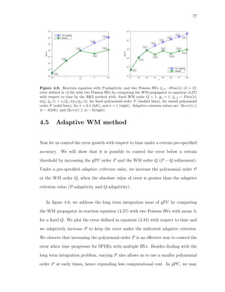

![79
us consider the Burgers equation as an example to compare the complexity of WM
and gPC.
4.6.1 Burgers equation with one RV
To compare WM and gPC methods for Burgers equation with one RV (ξ ∼ Pois(λ)),
we simply write the gPC and WM propagators separately and compare how they
differ from each other. We consider this equation:
ut + uux = νuxx + σc1(ξ; λ), x ∈ [−π, π]. (4.36)
The gPC propagator for this problem is:
∂ˆuk
∂t
+
P
m,n=0
ˆum
∂ˆun
∂x
< cmcnck >= ν
∂2
ˆuk
∂x2
+ σδ1k, k = 0, 1, ..., P. (4.37)
where < cmcnck >= S
dΓ(ξ)ck(ξ)cm(ξ)cn(ξ).
The WM propagator for this problem is:
∂˜uk
∂t
+
Q
p=0
P
i=0
˜ui
∂˜uk+2p−i
∂x
Ki,k+2p−i,Q = ν
∂2
˜uk
∂x2
+ σδ1k, k = 0, 1, ..., P. (4.38)
The only difference between gPC and WM propagators is between the term
P
m,n=0 ˆum
∂ˆun
∂x
< cmcnck > in gPC and the term Q
p=0
P
i=0 ˜ui
∂˜uk+2p−i
∂x
Ki,k+2p−i,p in
WM. Assuming that we are going to solve equations (4.37) and (4.38) with the same
time stepping scheme and the same spatial discretization, for each time step, let us
also assume that the computational complexity of computing one term like ˆui
∂ˆuj
∂x
is](https://image.slidesharecdn.com/thesis-150401122906-conversion-gate01/85/Thesis-100-320.jpg)
![80
α, while the complexity for the rest of the linear terms is 1.
Under this assumption, in equation (4.37) for gPC, we have (P + 1) equations
in the system, each one with complexity 1 + (P + 1)2
α, and therefore the total
complexity is (P + 1)[1 + (P + 1)2
α].
In equation (4.38) for WM, we still have (P + 1) equations in the system. By
denoting the number of terms like ˜ui
∂˜uj
∂x
in the whole WM propagator as C(P, Q), the
total complexity will be (P + 1) + C(P, Q)α, and we compute C(P, Q) numerically.
We demonstrate how to count C(P, Q), when P = 4, Q = 1/2 in figure 4.10: there
are five 4 × 4 grids, for k = 0, 1, 2, 3, 4 respectively for ˜ui
∂˜uj
∂x
in all the five equations
in the WM propagator. The horizontal axis represents the index i for ˜ui and the
vertical axis represents the index j for
∂˜uj
∂x
. We marked the terms like ˜ui
∂˜uj
∂x
in
the k-th equation in the WM propagator by drawing a circle at the (i, j) dot on
the k-th grid. In this way we may visualize the nonlinear terms in the propagator
and hence visualize the main computational complexity. In the WM method for
P = 4, Q = 1/2, only the circled dots are considered in the propagator, however
in the gPC method for P = 4, all the dots on the five grids are considered in the
propagator. Hence, we can see how many fewer terms like ˆui
∂ˆuj
∂x
we need to consider
in WM comparing to gPC.
When P is sufficiently large, the ratio for complexity of WM to gPC is approx-
imately C(P,Q)
(P+1)3 , ignoring lower order terms on P. Since we observed in Figures 4.5
and 4.6 that when Q = P −1, the errors computed from WM propagators are at the
same accuracy level as from gPC propagators, we calculate the ratio of complexity
between WM and gPC for Burgers equation with one RV C(P,Q=P−1)
(P+1)3 when Q = P −1](https://image.slidesharecdn.com/thesis-150401122906-conversion-gate01/85/Thesis-101-320.jpg)

![82
4.6.2 Burgers equation with d RVs
Now suppose we are going to solve the Burgers equation with d RVs (each RV ξi has
polynomial expansion order Pi and WM order Qi):
ut + uux = νuxx + σcm1 (ξ1)...cmd
(ξd), x ∈ [−π, π]. (4.40)
By gPC, we will have Πd
i=1(Pi + 1) equations in the propagator, and if Pi are all
equal to P, there will be (P + 1)d
equations in the gPC propagator. We will have
(Πd
i=1(Pi + 1))(Πd
i=1(Pi + 1)2
) terms like ˆuk
∂ˆuj
∂x
. When all the RVs are having the
same P, this number is (P + 1)3d
.
By WM, we will still have the same number of equations in the propagator
system, but the number of terms like ˆuk
∂ˆuj
∂x
is Πd
i=1C(Pi, Qi). Let us assume all the
RVs having the same P and Q. This formula can be written as (C(P, Q))d
.
When P is sufficiently large (for simplicity we assume Pi = P, Qi = Q for all
i = 1, 2, ..., d), the ratio for complexity of WM to gPC is approximately C(P,Q)d
(P+1)3d ,
ignoring lower order terms on P. We computed the ratio of complexity in figure 4.11
for d = 2, 3.
Besides figure 4.11, we also want to point out the following observation. From
figure 4.5 we observed numerically that when Q ≥ P −1, the error from WM method
with polynomial order P is at the same order as the error from gPC with polynomial
order P. So let us consider the computational cost ratio C(P,Q)d
(P+1)3d between the two
methods for WM with order Q = P − 1, and gPC with order P, in table (4.2).
We conclude from figure 4.11 and table (4.2) that: 1) the larger the P, the bigger](https://image.slidesharecdn.com/thesis-150401122906-conversion-gate01/85/Thesis-103-320.jpg)

![84
the cost ratio between WM to gPC (C(P,Q)d
(P+1)3d ); 2) the higher the dimensions, for the
same order P and Q, the lower the ratio C(P,Q)d
(P+1)3d . In other words, the higher the
dimensions, the less WM is going to cost than gPC for the same accuracy.
4.7 Conclusions
We presented a new Wick-Malliavin expansion to approximate polynomial non-
linear terms in SPDEs with random inputs of arbitrary discrete measure with fi-
nite moments, on which orthogonal polynomials can be constructed numerically
[127, 45, 54, 22, 125]. Specifically, we derived WM propagators for a stochastic
reaction equation and a Burgers equation in equation (4.27) and (4.32) with multi-
ple discrete RVs. The error was effectively improved by at least two to eight orders
of magnitude when the WM order Q was increased into a larger integer in figure 4.1
and 4.4. Linear and nonlinear SPDEs with multiple RVs were considered in figure
4.2 and 4.7 as the first step towards application of WM method to nonlinear SPDEs
with stochastic processes, such as Levy processes with jumps. We found the smallest
WM order Q for gPC polynomial order P in WM method to be Q = P − 1 in order
to achieve the same order of magnitude of error in gPC with polynomial order P or
PCM with (P + 1) collocation points, by computing the Burgers equation with one
Poisson RV in figure 4.5. When Q was larger than (P −1), the error remained almost
constant as in figure 4.6. We proposed an adaptive WM method in section 3.5, by
increasing the gPC order P and the WM order Q as a possible solution to control
the error growth in long-term integration in gPC, shown in figure 4.8 and 4.9. With
Q = P − 1 we estimated and compared the computational complexity between the
WM method and gPC for a stochastic Burgers equation with d RVs in section 3.5.
The WM method required much less computational complexity than gPC, especially](https://image.slidesharecdn.com/thesis-150401122906-conversion-gate01/85/Thesis-105-320.jpg)


![87
We develop new probabilistic and deterministic approaches for moment statistics of
stochastic partial differential equations (SPDEs) with pure jump tempered α-stable
(TαS) L´evy processes. With the CP approximation or the series representation of
the TαS process, we simulate the moment statistics of stochastic reaction-diffusion
equations with additive TαS white noises by the probability collocation method
(PCM) and the Monte Carlo (MC) method. PCM is shown to be more efficient and
accurate than MC in relatively low dimensions. Then as an alternative approach,
we solve the generalized Fokker-Planck (FP) equation that describes the evolution
of the density for stochastic overdamped Langevin equations to obtain the density
and the moment statistics for the solution following two different approaches. First,
we solve an integral equation for the density by approximating the TαS processes as
CP processes; second, we directly solve the tempered fractional PDE (TFPDE). We
show that the numerical solution of TFPDE achieves higher accuracy than PCM at
a lower cost and we also demonstrate agreement between the histogram from MC
and the density from the TFPDE.
5.1 Literature review of L´evy flights
The Kolmogorov scaling law of turbulences [84] assumes the turbulence as a stochas-
tic Gaussian process in small scales [146]. However, experimental data shows that
dissipation quantities become more non-Gaussian when the scale decreased and when
the Reynolds number increased [15]. At finite Reynolds numbers, non-Guassianness
was observed in velocity profiles [163], pressure profiles [160], and acceleration pro-
files [133]. Experimentally, L´evy flights from one vortex to another, sticking events
on one vortex, and power-law growth with time in the variance of displacement was
observed on a tracer particle in a time-periodic laminar flow [151]. The complimen-](https://image.slidesharecdn.com/thesis-150401122906-conversion-gate01/85/Thesis-108-320.jpg)
![88
tary sticking events and L´evy flights are known as intermittency [132]. Theoretically,
by assuming a uniform distribution of vortices in R3
, the velocity profile of the frac-
tal turbulence [102] is shown to be a stable distribution with characteristic exponent
D/2 [155], where D is the fractal dimension of the turbulence [103]. However, L´evy
flights are not directly applicable to real dynamical processes of turbulence [147].
One must consider the time spent on the completion of jumps from one vortex to
another in the L´evy walk model [145, 146]. The Richardson’s 4/3 law of turbulence
is derived from the L´evy walk model and a memory function based on Kolmogorov
scaling [146], where that derivation from the L´evy flight model has been unsatis-
factory [111]. L´evy flights are related to the symmetry of the dynamic system in
the phase space [147]: arbitrary weak perturbations (such as non-uniformity in tem-
perature, Ekman pumping, and finite-size particle effects) of quasisymmetric steady
flows destroy the separatrix grids and generate stochastic webs of finite thickness
(for streamlines and velocity fields [176]), where the streamlines randomly travel at
the cross-sections on the webs from one stable region (island) to another in pre-
turbulent states [17]. The first indirect experimental evidence of L´evy flights/walks
is observed from the self-similarity (of stable law) in the concentration profile of a
linear array of vortices, in the subdiffusion diffusion regime where the sticking dom-
inates, both around the vortices and in the boundary layers [26], in agreement with
the theory [131]. Direct experimental evidence of L´evy flights/walks and superdif-
fusion, where the L´evy flights dominate, is observed on a large number of tracers
in a two-dimensional flow [151]: in pre-turbulent states, the more random the flow,
the more frequent and random the tracer switches between the sticking events and
the L´evy flights; in turbulence, tracers wander so erratically that no flights can be
defined [150].](https://image.slidesharecdn.com/thesis-150401122906-conversion-gate01/85/Thesis-109-320.jpg)
![89
5.2 Notation
Lt, ηt L´evy processes
(c, λ, α) coefficients in tempered α-stable distributions (TαS)
N(t, U) Poisson random measure
I indicator function
E expectation
Γ gamma function
ν L´evy measure
˜N compensated Poisson random measure
Qcp number of truncations in the compound Poisson approximation
Qs number of truncations in the series representation
F cumulative distribution function
f probability density function
s number of samples in Monte Carlo simulation (MC)
γinc incomplete gamma function
d number of quadrature points in probability collocation methods (PCM)
Sk characteristic function of a L´evy process
−∞Dα
x left Riemann-Liouville fractional derivative
xDα
+∞ right Riemann-Liouville fractional derivative
−∞Dα,λ
x left Riemann-Liouville tempered fractional derivative
xDα,λ
+∞ right Riemann-Liouville tempered fractional derivative
5.3 Stochastic models driven by tempered stable
white noises
We develop and compare different numerical methods to solve two stochastic models
with tempered α-stable (TαS) L´evy white noises: a reaction-diffusion equation and
an overdamped Langevin equation with TαS white noises, including stochastic simu-
lation methods such as the MC [33, 128] and the PCM [8, 169]. We also simulate the
density of the overdamped Langevin equation through its generalized FP equation
formulated as TFPDE.](https://image.slidesharecdn.com/thesis-150401122906-conversion-gate01/85/Thesis-110-320.jpg)
![90
We first solve the following stochastic reaction-diffusion model via stochastic
simulation methods (MC and PCM) in the Itˆo sense:
du(t, x; ω) = (∂2u
∂x2 + µu)dt + dLt(ω), x ∈ [0, 2]
u(t, 0) = u(t, 2) periodic boundary condition
u(0, x) = u0(x) = sin(π
2
x) initial condition
(5.1)
where Lt(ω) is one-dimensional TαS process (also known as CGMY process in fi-
nance) [27, 28].
The second model is one-dimensional stochastic overdamped Langevin equation
in the Itˆo sense [36, 72]:
dx(t; ω) = −σx(t; ω)dt + dLt(ω), x(0) = x0, (5.2)
where Lt(ω) is also a one-dimensional TαS process. It describes an overdamped
particle in an external potential driven by additive TαS white noise. This equation
was introduced in [91] to describe the stochastic dynamics in fluctuating environ-
ments for Gaussian white noise, such as classical mechanics [61], biology [70], and
finance [33]. When Lt(ω) is a L´evy process, the solution is a Markov process and
its probability density satisfies a closed equation such as the differential Chapman-
Kolmogorov equation [53] or the generalized FP equation [137]. When Lt(ω) is a
TαS L´evy process, the corresponding generalized FP equation is a TFPDE [36].](https://image.slidesharecdn.com/thesis-150401122906-conversion-gate01/85/Thesis-111-320.jpg)
![91
5.4 Background of TαS processes
TαS processes were introduced in statistical physics to model turbulence, e.g., the
truncated L´evy flight model [85, 106, 121], and in mathematical finance to model
stochastic volatility, e.g., the CGMY model [27, 28]. Here, we consider a symmet-
ric TαS process (Lt) as a pure jump L´evy martingale with characteristic triplet
(0, ν, 0) [19, 143] (no drift and no Gaussian part). The L´evy measure is given by [33]
1
:
ν(x) =
ce−λ|x|
|x|α+1
, 0 < α < 2. (5.3)
This L´evy measure can be interpreted as an Esscher transformation [57] from that
of a stable process with exponential tilting of the L´evy measure. The parameter
c > 0 alters the intensity of jumps of all given sizes; it changes the time scale of
the process. Also, λ > 0 fixes the decay rate of big jumps, while α determines the
relative importance of smaller jumps in the path of the process2
. The probability
density for Lt at a given time is not available in a closed form (except when α = 1
2
3
).
The characteristic exponent for Lt is [33]:
Φ(s) = s−1
log E[eisLs
] = 2Γ(−α)λα
c[(1 −
is
λ
)α
− 1 +
isα
λ
], α = 1, (5.4)
where Γ(x) is the Gamma function and E is the expectation. By taking the deriva-
tives of the characteristic exponent we obtain the mean and variance:
E[Lt] = 0, V ar[Lt] = 2tΓ(2 − α)cλα−2
. (5.5)
1
In a more generalized form, L´evy measure is ν(x) = c−e−λ−|x|
|x|α+1 Ix<0 + c+e−λ+|x|
|x|α+1 Ix>0. We may
have different coefficients c+, c−, λ+, λ− on the positive and the negative jump parts.
2
In the case when α = 0, Lt is the gamma process.
3
See inverse Gaussian processes.](https://image.slidesharecdn.com/thesis-150401122906-conversion-gate01/85/Thesis-112-320.jpg)
![92
In order to derive the second moments for the exact solutions of Equations (5.1) and
(5.2), we introduce the Itˆo isometry. The jump of Lt is defined by Lt = Lt − Lt− .
We define the Poisson random measure N(t, U) as [71, 119, 123]:
N(t, U) =
0≤s≤t
I Ls∈U , U ∈ B(R0), ¯U ⊂ R0. (5.6)
Here R0 = R{0}, and B(R0) is the σ-algebra generated by the family of all Borel
subsets U ⊂ R, such that ¯U ⊂ R0; IA is an indicator function. The Poisson random
measure N(t, U) counts the number of jumps of size Ls ∈ U at time t. In order
to introduce the Itˆo isometry, we define the compensated Poisson random measure
˜N [71] as:
˜N(dt, dz) = N(dt, dz) − ν(dz)dt = N(dt, dz) − E[N(dt, dz)]. (5.7)
The TαS process Lt (as a martingale) can be also written as:
Lt =
t
0 R0
z ˜N(dτ, dz). (5.8)
For any t, let Ft be the σ-algebra generated by (Lt, ˜N(ds, dz)), z ∈ R0, s ≤ t. We
define the filtration to be F = {Ft, t ≥ 0}. If a stochastic process θt(z), t ≥ 0, z ∈ R0
is Ft-adapted, we have the following Itˆo isometry [119]:
E[(
T
0 R0
θt(z) ˜N(dt, dz))2
] = E[
T
0 R0
θ2
t (z)ν(dz)dt]. (5.9)
Equations (5.1) and (5.2) are understood in the Itˆo sense. The solutions are stochas-
tic Itˆo integrals over the TαS processes Lt [135], such as
T
0
f(t)dLt, with the L´evy
measure given in Equation (5.3). Thus, by applying Equation (5.8), the second](https://image.slidesharecdn.com/thesis-150401122906-conversion-gate01/85/Thesis-113-320.jpg)
![93
moment can be derived using the L´evy measure:
E[(
T
0
f(t)dLt)2
] = E[(
T
0 R0
f(t)z ˜N(dt, dz))2
] = E[
T
0 R0
f2
(t)z2
ν(dz)dt].
(5.10)
Both Equations (5.1) and (5.2) contain an additive white noise ˙Lt of a TαS process.
Details of white noise theory for L´evy processes with applications to SPDEs and
finance can be found in [18, 120, 96, 97, 124]. The white noise of a Poisson random
measure takes values in a certain distribution space. It is constructed via a chaos
expansion for L´evy processes with kernels of polynomial type [120], and defined as
a chaos expansion in terms of iterated integrals with respect to the compensated
Poisson measure ˜N(dt, dz) [74].
For simulations of TαS L´evy processes, we do not know the distribution of incre-
ments explicitly [33], but we may still simulate the trajectories of TαS processes by
the random walk approximation [10]. However, the random walk approximation does
not identify the jump time and size of the large jumps precisely [139, 140, 141, 142].
In the heavy tailed case, large jumps contribute more than small jumps in functionals
of a L´evy process. Therefore, in this case, we have mainly used two other ways to sim-
ulate the trajectories of a TαS process numerically: CP approximation [33] and series
representation [140]. In the CP approximation, we treat the jumps smaller than a
certain size δ by their expectation, and treat the remaining process with larger jumps
as a CP process [33]. There are six different series representations of L´evy jump pro-
cesses. They are the inverse L´evy measure method [44, 82], LePage’s method [92],
Bondesson’s method [23], thinning method [140], rejection method [139], and shot
noise method [140, 141]. In this paper, for TαS processes, we will use the shot noise
representation for Lt as a series representation method because the tail of L´evy mea-
sure of a TαS process does not have an explicit inverse [142]. Both the CP and the
series approximation converge slowly when the jumps of the L´evy process are highly](https://image.slidesharecdn.com/thesis-150401122906-conversion-gate01/85/Thesis-114-320.jpg)
![94
concentrated around zero, however both can be improved by replacing the small
jumps via Brownian motions [6]. The α-stable distribution was introduced to model
the empirical distribution of asset prices [104], replacing the normal distribution.
The empirical distribution of asset prices is not always in a stable distribution or a
normal distribution. The tail is heavier than a normal distribution and thinner than
a stable distribution [20]. Therefore, the TαS process was introduced as the CGMY
model to modify the Black and Scholes model.
In the past literature, the simulation of SDEs or functionals of TαS processes
was mainly done via MC [128]. MC for functionals of TαS processes is possible after
a change of measure that transform TαS processes into stable processes [130].
5.5 Numerical simulation of 1D TαS processes
In general there are three ways to generate a L´evy process [140]: random walk ap-
proximation, series representation and CP approximation. For a TαS process, the
distribution of increments is not explicitly known (except for α = 1/2) [33]. There-
fore, in the sequel we discuss the CP approximation and the series representation for
a TαS process.
5.5.1 Simulation of 1D TαS processes by CP approximation
In the CP approximation, we simulate the jumps larger than δ as a CP process
and replace jumps smaller than δ by their expectation as a drift term [33]. Here
we explain the method to approximate a TαS subordinator Xt (without a Gaussian](https://image.slidesharecdn.com/thesis-150401122906-conversion-gate01/85/Thesis-115-320.jpg)
![95
part and a drift) with the L´evy measure ν(x) = ce−λx
xα+1 Ix>0 (positive jumps only); this
method can be generalized to a TαS process with both positive and negative jumps.
The CP approximation Xδ
t for this TαS subordinator Xt is:
Xt ≈ Xδ
t =
s≤t
XsI Xs≥δ+E[
s≤t
XsI Xs<δ] =
∞
i=1
Jδ
i It≤Ti
+bδ
t ≈
Qcp
i=1
Jδ
i It≤Ti
+bδ
t,
(5.11)
We introduce Qcp here as the number of jumps occurred before time t. The first
term ∞
i=1 Jδ
i It≤Ti
is a compound Poisson process with jump intensity
U(δ) = c
∞
δ
e−λx
dx
xα+1
(5.12)
and jump size distribution pδ
(x) = 1
U(δ)
ce−λx
xα+1 Ix≥δ for Jδ
i . The jump size random
variables (RVs) Jδ
i are generated via the rejection method [37]. Here is a brief
description of an algorithm to generate RVs with distribution pδ
(x) = 1
U(δ)
ceλx
xα+1 Ix≥δ
for CP approximation, by the rejection method. The distribution pδ
(x) can be
bounded by
pδ
(x) ≤
δ−α
e−λδ
αU(δ)
fδ
(x), (5.13)
where fδ
(x) = αδ−α
xα+1 Ix≥δ. The algorithm is [33, 37]:
REPEAT
Generate RVs W and V : independent and uniformly distributed on [0, 1]
Set X = δW−1/α
Set T = fδ(X)δ−αe−λδ
pδ(X)αU(δ)
UNTIL V T ≤ 1
RETURN X .
Here, Ti is the i-th jump arrival time of a Poisson process with intensity U(δ).
The accuracy of CP approximation method can be improved by replacing the smaller](https://image.slidesharecdn.com/thesis-150401122906-conversion-gate01/85/Thesis-116-320.jpg)
![96
jumps by a Brownian motion [6], when the growth of the L´evy measure near zero
is fast. The second term functions as a drift term, bδ
t, resulted from truncating
the smaller jumps. The drift is bδ
= c
δ
0
e−λxdx
xα . This integration diverges when
α ≥ 1, therefore the CP approximation method only applies to TαS processes with
0 < α < 1. In this paper, both the intensity U(δ) and drift bδ
are calculated
via numerical integrations with Gauss-quadrature rules [54] with a specified relative
tolerance (RelTol) 4
. In general, there are two algorithms to simulate a compound
Poisson process [33]: the first method is to simulate the jump time Ti by exponentially
distributed RVs and take the number of jumps Qcp as large as possible; the second
method is to first generate and fix the number of jumps, then generate the jump time
by uniformly distributed RVs on [0, t]. Algorithms for simulating a CP process (the
second kind) with intensity and the jump size distribution in their explicit forms are
known on a fixed time grid [33]. Here we describe how to simulate the trajectories of a
CP process with intensity U(δ) and jump size distribution νδ(x)
U(δ)
, on a simulation time
domain [0, T] at time t. The algorithm to generate sample paths for CP processes is
given below.
• Simulate an RV N from Poisson distribution with parameter U(δ)T, as the
total number of jumps on the interval [0, T].
• Simulate N independent RVs, Ti, uniformly distributed on the interval [0, T],
as jump times.
• Simulate N jump sizes, Yi with distribution νδ(x)
U(δ)
.
• Then the trajectory at time t is given by N
i=1 ITi≤tYi.
In order to simulate the sample paths of a symmetric TαS process with a L´evy
4
The RelTol of numerical integration is defined as |q−Q|
|Q| , where q is the computed value of the
integral and Q is the unknown exact value.](https://image.slidesharecdn.com/thesis-150401122906-conversion-gate01/85/Thesis-117-320.jpg)
![97
measure given in Equation (5.3), we generate two independent TαS subordinators
via the CP approximation and subtract one from the other. The accuracy of the CP
approximation is determined by the jump truncation size δ.
5.5.2 Simulation of 1D TαS processes by series representa-
tion
Let { j}, {ηj}, and {ξj} be sequences of i.i.d. RVs such that P( j = ±1) = 1/2, ηj ∼
Exponential(λ), and ξj ∼Uniform(0, 1). Let {Γj} be arrival times in a Poisson
process with rate one. Let {Uj} be i.i.d. uniform RVs on [0, T]. Then, a TαS
process Lt with L´evy measure given in Equation (5.3) can be represented as [142]:
Lt =
+∞
j=1
j[(
αΓj
2cT
)−1/α
∧ ηjξ
1/α
j ]I{Uj≤t}, 0 ≤ t ≤ T. (5.14)
Equation (5.14) converges almost surely as uniformly in t [139]. In numerical simu-
lations, we truncate the series in Equation (5.14) up to Qs terms. The accuracy of
series representation approximation is determined by the number of truncations Qs.
5.5.3 Example: simulation of inverse Gaussian subordina-
tors by CP approximation and series representation
In order to compare the numerical performance of CP approximation and series
representation of TαS processes, we simulate the trajectories of an inverse Gaussian
(IG) subordinator by the two methods. An IG subordinator is a TαS subordinator](https://image.slidesharecdn.com/thesis-150401122906-conversion-gate01/85/Thesis-118-320.jpg)
![98
with a L´evy measure (with one-sided jumps, α = 1/2) as:
νIG =
ce−λx
x3/2
Ix>0. (5.15)
The probability density function (pdf) at time t for an IG subordinator is known to
be [33]:
pt(x) =
ct
x3/2
e2ct
√
πλ
e−λx−πc2t2/x
, x > 0. (5.16)
We perform the one-sample Kolmogorov-Smirnov statistic (K-S test) [107] between
the empirical cumulative distribution function (CDF) and the exact reference CDF:
KS = sup
x
|Fem(x) − Fex(x)|, x ∈ supp(F). (5.17)
This one-sample K-S test quantifies a distance between the exact inverse Gaussian
process and the approximated one (by the CP approximation or the series represen-
tation).
In Figures 5.1 and 5.2, we plot the empirical histograms (with the area normal-
ized to one) of an IG subordinator at time t, simulated via the CP approximation
with different small jump truncation sizes δ (explained in Section 2.1) and via the
series representation with different numbers of truncations in the series Qs (explained
in Section 2.2), against the reference PDF in Equation (5.16). We observe that the
empirical histograms fit the reference PDF better when δ → 0 in the CP approxima-
tion in Figure 5.1 and when Qs increases in the series representation. The quality of
fitting is shown quantitatively via the K-S test values given in each plot.
In both Figures 5.1 and 5.2, we run one million samples on 1000 bins for each
histogram (known as the square-root choice [159]). We zoom in and plot the parts
of histograms on [0, 1.8] to examine how smaller jumps are captured. We observe](https://image.slidesharecdn.com/thesis-150401122906-conversion-gate01/85/Thesis-119-320.jpg)
![99
0 1 2 3 4 5
0
20
40
60
80
100
x
p
t
(x)
CP =0.1
reference PDF
0 0.5 1 1.5
0
0.5
1
1.5
2
2.5
CP =0.1
reference PDF
KS=0.152843
0 1 2 3 4
0
0.5
1
1.5
2
2.5
3
3.5
x
p
t
(x)
CP =0.02
reference PDF
0 0.5 1 1.5
0
0.5
1
1.5
2
2.5
CP =0.02
reference PDF
KS=0.009250
0 1 2 3 4
0
0.5
1
1.5
2
x
p
t
(x)
CP =0.005
reference PDF
0 0.5 1 1.5
0
0.5
1
1.5
2
CP =0.005
reference PDF
KS=0.003414
Figure 5.1: Empirical histograms of an IG subordinator (α = 1/2) simulated via
the CP approximation at t = 0.5: the IG subordinator has c = 1, λ = 3; each simulation contains
s = 106
samples (we zoom in and plot x ∈ [0, 1.8] to examine the smaller jumps approximation);
they are with different jump truncation sizes as δ = 0.1 (left, dotted, CPU time 1450s), δ = 0.02
(middle, dotted, CPU time 5710s), and δ = 0.005 (right, dotted, CPU time 38531s). The reference
PDFs are plotted in red solid lines; the one-sample K-S test values are calculated for each plot; the
RelTol of integration in U(δ) and bδ
is 1 × 10⁻⁸
. These runs were done on Intel (R) Core (TM)
i5-3470 CPU @ 3.20 GHz in Matlab.
0 1 2 3 4 5
0
0.5
1
1.5
2
2.5
x
p
t
(x)
series rep Q=10
reference PDF
0 0.5 1 1.5
0
0.5
1
1.5
2
2.5
series rep Q=10
reference PDF
KS=0.360572
0 1 2 3 4 5
0
0.5
1
1.5
2
x
p
t
(x)
series rep Q=100
reference PDF
0 0.5 1 1.5
0
0.5
1
1.5
2
series rep Q=100
reference PDF
KS=0.078583
0 1 2 3 4
0
0.5
1
1.5
2
x
p
t
(x)
series rep Q=800
reference PDF
0 0.5 1 1.5 2
0
0.5
1
1.5
2
series rep Q=800
reference PDF
KS=0.040574
Figure 5.2: Empirical histograms of an IG subordinator (α = 1/2) simulated via
the series representation at t = 0.5: the IG subordinator has c = 1, λ = 3; each simulation is
done on the time domain [0, 0.5] and contains s = 106
samples (we zoom in and plot x ∈ [0, 1.8] to
examine the smaller jumps approximation); they are with different number of truncations in the
series as Qs = 10 (left, dotted, CPU time 129s), Qs = 100 (middle, dotted, CPU time 338s), and
Qs = 1000 (right, dotted, CPU time 2574s). The reference PDFs are plotted in red solid lines; the
one-sample K-S test values are calculated for each plot. These runs were done on Intel (R) Core
(TM) i5-3470 CPU @ 3.20 GHz in Matlab.](https://image.slidesharecdn.com/thesis-150401122906-conversion-gate01/85/Thesis-120-320.jpg)
![100
that in both Figures 5.1 and 5.2 when δ is large or Qs is small, the distribution of
small jumps is not well approximated. Therefore, both methods suffer from accuracy
if smaller jumps have a big contribution to the solution of SPDEs, e.g., when α or
λ is large. Furthermore, when δ is large in the CP approximation (see δ = 0.1 in
Figure 5.1), the big jumps are well approximated although the small ones are not;
when Qs is small in the series representation, neither big or small jumps are not well
approximated (see Qs = 10 in Figure 5.2). When the cost is limited, this shows an
advantage of using the CP approximation, when big jumps have a larger contribution
to the solution of SPDEs.
5.6 Simulation of stochastic reaction-diffusion model
driven by TαS white noises
In this section, we will provide numerical results for solving the stochastic reaction-
diffusion Equation (5.1). We will perform and compare four stochastic simulation
methods to obtain the statistics: MC with CP approximation (MC/CP), MC with
series representation (MC/S), PCM with CP approximation (MC/CP), and PCM
with series representation (PCM/S).
The integral form of Equation (5.1) is:
u(t, x) = eµt−π2
4
t
sin(
π
2
x) + eµt
t
0
e−µτ
dLτ , x ∈ [0, 2], (5.18)
where the stochastic integral is an Itˆo integral over a TαS process [135]. The mean
of the solution is
Eex[u(t, x)] = eµt−π2
4
t
sin(
π
2
x). (5.19)](https://image.slidesharecdn.com/thesis-150401122906-conversion-gate01/85/Thesis-121-320.jpg)
![101
By the Itˆo isometry [119] and Equation (5.19), the second moment of the solution is
Eex[u2
(t, x; ω)] = e2µt−π2
2
t
sin2
(
π
2
x) +
c 2
e2µt
µλ2−α
(1 − e−2µt
)Γ(2 − α). (5.20)
Let us define the L2 norm of the error in the second moment l2u2(t) to be
l2u2(t) =
||Eex[u2
(x, t; ω)] − Enum[u2
(x, t; ω)]||L2([0,2])
||Eex[u2(x, t; ω)]||L2([0,2])
, (5.21)
where Enum[u2
(x, t; ω)] is the second moment evaluated by numerical simulations.
5.6.1 Comparing CP approximation and series representa-
tion in MC
First we will compare the accuracy and convergence rate between MC/CP and MC/S
in solving (5.1) by MC. In MC, we generate the trajectories of Lt (a TαS process
with the Levy measure given in Equation (5.3)) on a fixed time grid with st the
number of time steps ({t0 = 0, t1, t2, ..., tst = T}). We solve Equation (5.1) via the
first-order Euler’s method [128] in the time direction with a time step t = tn+1
−tn
:
un+1
− un
= (
∂2
un
∂x2
+ µun
) t + (Ltn+1 − Ltn ). (5.22)
We discretize the space by Nx = 500 Fourier collocation points [66] on the domain
[0, 2].
In Table 5.1, we plot the l2u2 errors at a fixed time T versus the sample size s
by the MC/CP and the MC/S, for λ = 10 (upper) and for λ = 1 (lower, with a less
tempered tail). First for the cost, the MC/CP costs less CPU time than the MC/S,](https://image.slidesharecdn.com/thesis-150401122906-conversion-gate01/85/Thesis-122-320.jpg)
![102
e.g., when λ = 10 in Table 5.1, the MC/S with Qs = 10 and s = 65536 takes twice
the CPU time as the MC/CP with δ = 0.01 and s = 65536 even though the MC/CP
is more accurate. Second, to assess the accuracy of the methods, the MC/CP is more
accurate than MC/S even though it takes about half the CPU time, e.g. the MC/CP
with δ = 0.01 and the MC/S with Qs = 10. Third, we observe that decreasing δ
in the MC/CP to improve the accuracy is more effective with a small s when more
smaller jumps are present (larger λ). For example: when λ = 10, δ = 0.01 starts
to be more accurate than δ = 0.1 when s = 1024; when λ = 10, δ = 0.01 starts to
be more accurate than δ = 0.1 when s = 65536. This can be explained by the fact
that large jumps have a greater contribution to the solution and decreasing δ in the
MC/CP makes a great difference in sampling smaller jumps as in Figure 5.1.
Table 5.1: MC/CP vs. MC/S: error l2u2(T) of the solution for Equation (5.1) versus the number
of samples s with λ = 10 (upper) and λ = 1 (lower). T = 1, c = 0.1, α = 0.5, = 0.1, µ = 2
(upper and lower). Spatial discretization: Nx = 500 Fourier collocation points on [0, 2]; temporal
discretization: first-order Euler scheme in (5.22) with time steps t = 1 × 10⁻⁵
. In the CP
approximation: RelTol = 1 × 10⁻⁸
for integration in U(δ).
s (λ = 10) 256 1024 4096 16384 65536 262144
MC/S Qs = 10 3.9 × 10⁻³
6.0 × 10⁻⁴
1.6 × 10⁻⁴
6.8 × 10⁻⁵
2.3 × 10⁻⁵
3.5 × 10⁻⁶
MC/CP δ = 0.1 5.4 × 10⁻⁴
6.2 × 10⁻⁴
6.3 × 10⁻⁴
4.3 × 10⁻⁴
4.3 × 10⁻⁴
4.5 × 10⁻⁴
MC/CP δ = 0.01 3.6 × 10⁻⁴
1.8 × 10⁻⁵
9.8 × 10⁻⁵
1.3 × 10⁻⁵
3.5 × 10⁻⁶
2.0 × 10⁻⁵
s (λ = 1) 256 1024 4096 16384 65536 262144
MC/S Qs = 10 1.7 × 10⁻²
1.4 × 10⁻²
6.1 × 10⁻³
7.6 × 10⁻³
4.4 × 10⁻³
6.6 × 10⁻⁴
MC/CP δ = 0.1 1.8 × 10⁻³
4.9 × 10⁻³
2.4 × 10⁻³
2.5 × 10⁻³
5.1 × 10⁻⁴
2.7 × 10⁻⁴
MC/CP δ = 0.01 8.6 × 10⁻³
3.8 × 10⁻³
5.8 × 10⁻³
2.0 × 10⁻³
1.1 × 10⁻⁴
3.6 × 10⁻⁵
5.6.2 Comparing CP approximation and series representa-
tion in PCM
Next, we will compare the accuracy and efficiency between PCM/CP and PCM/S
in solving (5.1). In order to evaluate the moments of solutions, PCM [169], as](https://image.slidesharecdn.com/thesis-150401122906-conversion-gate01/85/Thesis-123-320.jpg)
![103
an integration method on the random space, is based on the Gauss-quadrature
rules [54]. Suppose the solution is a function of a finite number of independent RVs
({Y 1
, Y 2
, ..., Y n
)}) as v(Y 1
, Y 2
, ..., Y n
), the m-th moment of the solution is evaluated
by
E[vm
(Y 1
, Y 2
, ..., Y n
)] =
d1
i1=1
...
dn
in=1
vm
(y1
i1
, y2
i2
, ..., yn
in
)w1
i1
...wn
in
, (5.23)
where wj
ij
and yj
ij
are the ij-th Gauss-quadrature weight and collocation point for
Y j
respectively. The simulations are run on (Πn
i=1di) deterministic sample points
(y1
i1
, ..., yn
in
) in the n-dimensional random space. In the CP approximation, the TαS
process Lt is approximated via Lt ≈
Qcp
i=1 Jδ
i It≤Ti
+ bδ
t, where Qcp is the number of
jumps we consider. As we mentioned in Section 2.1 there are two ways to simulate a
compound Poisson process. Here we treat the number of jumps Qcp as a modeling pa-
rameter by the CP approximation and simulate the time between two jumps Ti+1 −Ti
by exponentially distributed RVs with intensity U(δ). The PCM/CP method con-
tains two parameters: the jump truncation size δ and the number of jumps we
consider Qcp. Therefore, the PCM/CP simulations of problem (5.1) are run on the
collocation points for RVs Jδ
i and Ti in the 2Qcp-dimensional random space (with
d2Qcp
sample points); Qcp is the number of jumps truncated. In the series representa-
tion, the TαS process Lt is approximated via Lt ≈ Qs
j=1 j[(
αΓj
2cT
)−1/α
∧ ηjξ
1/α
j ]I{Uj≤t}
on the simulation domain [0, T]. To reduce the number of RVs (therefore, to de-
crease the number of dimensions in the random space), we calculate the distribution
of [(
αΓj
2cT
)−1/α
∧ηjξ
1/α
j ] for a fixed j and treat it as one RV for each j. The distribution
of Aj is calculated by the following:
FAj
(A) = P (
αΓj
2cT
)−1/α
≤ A = P Γj ≥
2cT
αAα
=
+∞
2cT
αAα
e−x
x−1+j
Γ(j)
dx, (5.24)](https://image.slidesharecdn.com/thesis-150401122906-conversion-gate01/85/Thesis-124-320.jpg)
![104
Therefore, the distribution of A is
fAj
(A) =
dFA
dA
=
2cT
Γ(j)Aα+1
e− 2cT
αAα
2cT
αAα
−1+j
. (5.25)
The distribution of Bj is derived by product distribution:
fBj
(B) = αλ
1
0
xα−2
e−λB/x
dx = (αλ)(λB)α−1
∞
λB
t−α
e−t
dt (5.26)
when α = 1, it can be written as incomplete Gamma functions.
Therefore, the distribution of [Aj ∧ Bj] is given by
fAj∧Bj
(x) = fAj
(x) 1 − FBj
(x) + fBj
(x) 1 − FAj
(x) . (5.27)
When 0 < α < 1,
fAj∧Bj
(x) =
α
xΓ(j)
e−t
tj
|t= 2cT
αxα
αΓ(1 − α)λα
+∞
x
(1 − γinc(λz, 1 − α))zα−1
dz
+ αΓ(1 − α)λα
(1 − γinc(λx, 1 − α)xα−1
) γinc(
2cT
αxα
, j).
(5.28)
When 1 < α < 2,
fAj∧Bj
(x) =
α
xΓ(j)
e−t
tj
|t= 2cT
αxα
+∞
x
fBj
(z)dz + fBj
(x)γinc(
2cT
αxα
, j). (5.29)](https://image.slidesharecdn.com/thesis-150401122906-conversion-gate01/85/Thesis-125-320.jpg)
![105
Here the incomplete Gamma function γinc(a, b) is defined as:
γinc(a, b) =
1
Γ(a)
b
0
e−t
ta−1
dt. (5.30)
Therefore, the PCM/S simulations under the series representation are run on the
quadrature points for RVs j, [(
αΓj
2cT
)−1/α
∧ ηjξ
1/α
j ], and Uj in the 3Qs-dimensional
random space (with d3Qs
sample points). In the sequel, we generate the stochastic
collocation points numerically based on the moments [125]. The stochastic colloca-
tion points are generated by the Gaussian quadrature rule [60]. Alternative methods
can also be used such as the Stieltjes’ method and the modified Chebyshev method
[55]. Here, we assume each RV has the same number of collocation points d.
However, typically for this problem (5.1) we only need d(Qcp + 1) sample points
in PCM/CP instead of d2Qcp
and only dQs sample points in PCM/S instead of d3Qs
.
Using the CP approximation given in Equation (5.11), the second moment of the
solution in (5.18) can be approximated by
E[u2
(t, x; ω)] ≈ e2µt−1
2
π2t
sin2
(
π
2
x) + 2
e2µt
E[(Jδ
1 )2
]
Qcp
i=1
E[e−2µTi
]. (5.31)
Using the series representation given in Equation (5.14), the second moment of the
solution in (5.18) can be approximated by
E[u2
(t, x; ω)] ≈ e2µt−1
2
π2t
sin2
(
π
2
x)+ 2
e2µt 1
2µT
(1−e−2µT
)
Qs
j=1
E[((
αΓj
2cT
)−1/α
∧ηjξ
1/α
j )2
].
(5.32)
Here we sample the moments of solution directly from Equation (5.31) for the
PCM/CP and Equation (5.32) for the PCM/S, therefore we significantly decrease the
sample size with the integral form of the solution in Equation (5.18). For example,](https://image.slidesharecdn.com/thesis-150401122906-conversion-gate01/85/Thesis-126-320.jpg)
![106
in this typical problem we may evaluate E[e−2µTi
] for each i separately in Equation
(5.31). Indeed, such reduction of the number of samples in the PCM method is pos-
sible whenever the following condition can be met. Suppose we have Q independent
R.V.s {Zi, i = 1, ..., Q}. If the expectation of a functional of {Zi, i = 1, ..., Q} is a
functional of expectation of some function of each Zi separately:
E[F(Z1, ..., Zd)] = G(E[f1(Z1)], ..., E[fd(Zd)]), (5.33)
we may evaluate each E[fi(Zi)] ‘separately’ via the PCM with d collocation points.
In this way, we reduce the number of samples from dQ
to dQ.
In Figure 5.3, we plot the l2u2(T) errors of the solution for Equation (5.1) versus
the number of jumps Qcp (via PCM/CP) or Qs (via PCM/S). In order to investigate
the Qcp and Qs convergence, we apply a sufficient number of collocation points for
each RV until the integration is up to a certain RelTol. We observe three things in
Figure 5.3.
1. For smaller values of Qs and Qcp, PCM/S is more accurate and converges faster
than PCM/CP, because bigger jumps contribute more to the solution and
PCM/S samples bigger jumps more efficiently than PCM/CP as we observed
in Figures 5.1 and 5.2.
2. For intermediate values of Qs and Qcp, the convergence rate of PCM/S slows
down but the convergence rate of PCM/CP speeds up, because the contribution
of smaller jumps starts to affect the accuracy since the PCM/CP samples the
smaller jumps faster than PCM/S.
3. For larger values of Qs and Qcp, both PCM/CP and PCM/S stop converging
due to their own limitations to achieve higher accuracy.](https://image.slidesharecdn.com/thesis-150401122906-conversion-gate01/85/Thesis-127-320.jpg)
![107
0 5 10 15 20 25 30 35
10
−18
10
−16
10
−14
10
−12
10
−10
10
−8
10
−6
Qcp
or Qs
l2u2(T=1)
PCM/CP =1×10⁻¹
PCM/CP =1×10
−2
PCM/CP =1×10⁻³
PCM/CP =1×10⁻⁴
PCM/CP =1×10⁻⁵
PCM/S
0 5 10 15 20 25 30 35
10
−15
10
−10
10
−5
Q
cp
or Q
s
l2u2(T=1)
PCM/CP =1×10⁻¹
PCM/CP =1×10
−2
PCM/CP =1×10⁻³
PCM/CP =1×10⁻⁴
PCM/CP =1×10
−5
PCM/S
Figure 5.3: PCM/CP vs. PCM/S: error l2u2(T) of the solution for Equation (5.1) versus the
number of jumps Qcp (in PCM/CP) or Qs (in PCM/S) with λ = 10 (left) and λ = 1 (right). T = 1,
c = 0.1, α = 0.5, = 0.1, µ = 2, Nx = 500 Fourier collocation points on [0, 2] (left and right). In
the PCM/CP: RelTol = 1 × 10⁻¹⁰
for integration in U(δ). In the PCM/S: RelTol = 1 × 10⁻⁸
for
the integration of E[((
αΓj
2cT )−1/α
∧ ηjξ
1/α
j )2
].
The limitations of PCM/CP and PCM/S are:
• in the PCM/CP when δ is small, the integration to calculate U(δ) = c
∞
δ
e−λxdx
xα+1
is less accurate because of the singularity of the integrand at 0;
• in the PCM/S, the density for the RV [(
αΓj
2cT
)−1/α
∧ηjξ
1/α
j ] in (5.14) for a greater
value of j requires more collocation points (d) to accurately approximate the
expectation of any functionals of [(
αΓj
2cT
)−1/α
∧ ηjξ
1/α
j ].
Within their own limitations (δ not too small, Qs not too large), the PCM/S achieves
higher accuracy than the PCM/CP, however it costs much more computational time
especially when the TαS process Lt contains more smaller jumps. For example,
when λ = 10 in Figure 5.3, to achieve the same accuracy of 10−11
, the PCM/S with
Qs = 10 costs more than 100 times of CPU time than the PCM/CP with Qcp = 30
and δ = 1 × 10⁻⁵
.](https://image.slidesharecdn.com/thesis-150401122906-conversion-gate01/85/Thesis-128-320.jpg)

![109
10
0
10
2
10
4
10
6
10
8
10
10
10
−4
10
−3
10
−2
10
−1
s
l2u2(T=1)
MC/CP
PCM/CP, d=2, s=d2Q
cp
PCM/CP, d=2, s=d(Q
cp
+1)
PCM/CP, d=3, s=d2Q
cp
PCM/CP, d=3, s=d(Qcp
+1)
10
0
10
5
10
10
10
15
10
−5
10
−4
10
−3
10
−2
10
−1
s
l2u2(T=1)
MC/S, Q
s
=10
PCM/S, d=2, s=d
3Q
s
PCM/S, d=3, s=d
3Q
s
PCM/S, d=2, s=dQ
s
PCM/S, d=3, s=dQ
s
Figure 5.4: PCM vs. MC: error l2u2(T) of the solution for Equation (5.1) versus the number
of samples s obtained by MC/CP and PCM/CP with δ = 0.01 (left) and MC/S with Qs = 10
and PCM/S (right). T = 1 , c = 0.1, α = 0.5, λ = 1, = 0.1, µ = 2 (left and right). Spatial
discretization: Nx = 500 Fourier collocation points on [0, 2] (left and right); temporal discretization:
first-order Euler scheme in (5.22) with time steps t = 1 × 10⁻⁵
(left and right). In both MC/CP
and PCM/CP: RelTol = 1 × 10⁻⁸
for integration in U(δ).
5.7 Simulation of 1D stochastic overdamped Langevin
equation driven by TαS white noises
In this section, we will present two methods to simulate the statistics for Equation
(5.2) by solving the corresponding generalized FP equation. In the first method,
we solve the density by approximating the TαS process Lt by a CP process, while
in the second method, we solve a TFPDE. We will compare these two FP equation
approaches with the previous MC and PCM methods via the empirical histograms
and errors of moments.](https://image.slidesharecdn.com/thesis-150401122906-conversion-gate01/85/Thesis-130-320.jpg)
![110
5.7.1 Generalized FP equations for overdamped Langevin
equations with TαS white noises
It is known that for any overdamped Langevin equation with a L´evy white noise ηt:
dx(t) = f(x(t), t)dt + dηt(ω), x(0) = x0, (5.34)
the PDF of the solution P(x, t) satisfies the following generalized FP equation [36]:
∂
∂t
P(x, t) = −
∂
∂x
f(x, t) P(x, t) + F−1
Pk(t) lnSk . (5.35)
Sk is the characteristic function (ch.f.) of the process ηt at time t = 1, as Sk =
E[e−ikη1
]. We define the Fourier transformation for a function v(x) as F{v(x)} =
vk =
+∞
−∞
dxe−ikx
v(x). Pk(t) is the ch.f. of x(t), as Pk(t) = E[e−ikx(t)
]. The inverse
Fourier transformation is defined as F−1
{vk(x)} = v = 1
2π
+∞
−∞
dxeikx
vk(x).
By the CP approximation with the jump truncation size δ of the TαS process Lt
for Equation (5.2), the density Pcp(x, t) of the solution x(t) satisfies [36]:
∂
∂t
Pcp(x, t) = σ − 2U(δ) Pcp(x, t) + σx
∂Pcp(x, t)
∂x
+
+∞
−∞
dyPcp(x − y, t)
ce−λ|y|
|y|α+1
(5.36)
with the initial condition Pcp(x, 0) = δ(x − x0), where U(δ) is defined in Equation
(5.12).
We also obtain the generalized FP equations as TFPDE for the density Pts(x, t)
directly from Equation (5.35) without approximating Lt by a CP process for Equa-
tion (5.2). Due to the fact that when 0 < α < 1 and 1 < α < 2, the ch.f.s for L1, Sk,
are in different forms, the density Pts(x, t) satisfies different equations for each case.](https://image.slidesharecdn.com/thesis-150401122906-conversion-gate01/85/Thesis-131-320.jpg)
![111
When 0 < α < 1, Sk = exp [−D{(λ + ik)α
− λα
}] [33, 109], where D = c
α
Γ(1−α),
Γ(t) =
+∞
0
xt−1
e−x
dx, the density Pts(x, t) satisfies:
∂
∂t
Pts(x, t) =
∂
∂x
σxPts(x, t) − D(α) −∞Dα,λ
x Pts(x, t) + xDα,λ
+∞Pts(x, t) , 0 < α < 1
(5.37)
with the initial condition Pts(x, 0) = δ(x−x0). The left and right Riemann-Liouville
tempered fractional derivatives are defined as [10, 109]:
−∞Dα,λ
x f(x) = e−λx
−∞Dα
x [eλx
f(x)] − λα
f(x), 0 < α < 1, (5.38)
and
xDα,λ
+∞f(x) = eλx
xDα
+∞[e−λx
f(x)] − λα
f(x), 0 < α < 1. (5.39)
In the above definitions, for α ∈ (n − 1, n) and f(x) (n − 1)-times continuously
differentiable on (−∞, +∞), −∞Dα
x and xDα
+∞ are left and right Riemann-Liouville
fractional derivatives defined as [10]:
−∞Dα
x f(x) =
1
Γ(n − α)
dn
dxn
x
−∞
f(ξ)
(x − ξ)α−n+1
dξ, (5.40)
xDα
+∞f(x) =
(−1)n
Γ(n − α)
dn
dxn
+∞
x
f(ξ)
(ξ − x)α−n+1
dξ. (5.41)
When 1 < α < 2, Sk = exp[D{(λ + ik)α
− λα
− ikαλα−1
}] [33, 109], where
D(α) = c
α(α−1)
Γ(2 − α), the density Pts(x, t) satisfies:
∂
∂t
Pts(x, t) =
∂
∂x
σxPts(x, t) + D(α) −∞Dα,λ
x Pts(x, t) + xDα,λ
+∞Pts(x, t) , 1 < α < 2
(5.42)
with the initial condition Pts(x, 0) = δ(x−x0). The left and right Riemann-Liouville](https://image.slidesharecdn.com/thesis-150401122906-conversion-gate01/85/Thesis-132-320.jpg)
![112
tempered fractional derivatives are defined as [10, 109]:
−∞Dα,λ
x f(x) = e−λx
−∞Dα
x [eλx
f(x)] − λα
f(x) − αλα−1
f (x), 1 < α < 2, (5.43)
and
xDα,λ
+∞f(x) = eλx
xDα
+∞[e−λx
f(x)] − λα
f(x)+αλα−1
f (x), 1 < α < 2. (5.44)
The left and right Riemann-Liouville fractional derivative −∞Dα
x and xDα
+∞ can
be numerically implemented via the Gr¨unwald-Letnikov finite difference form for
0 < α < 1 [108, 109, 129]:
−∞Dα
x f(x) = limh→0
+∞
j=0
1
hα Wjf(x − jh), 0 < α < 1;
xDα
+∞f(x) = limh→0
+∞
j=0
1
hα Wjf(x + jh), 0 < α < 1.
(5.45)
Here, −∞Dα
x and xDα
+∞ are implemented via the shifted Gr¨unwald-Letnikov finite
difference form for 1 < α < 2 [109, 129]:
−∞Dα
x f(x) = limh→0
+∞
j=0
1
hα Wjf(x − (j − 1)h), 1 < α < 2;
xDα
+∞f(x) = limh→0
+∞
j=0
1
hα Wjf(x + (j − 1)h), 1 < α < 2.
(5.46)
Note that Wk =
α
k
(−1)k
= Γ(k−α)
Γ(−α)Γ(k+1)
can be derived recursively via
W0 = 1, W1 = −α, Wk+1 = k−α
k+1
Wk. In the following numerical experiments, we
will solve equations (5.37) and (5.42) by the aforementioned first-order numerical
fractional finite difference scheme for spatial discretization on a sufficiently large do-
main [−L, L] and fully-implicit scheme for temporal discretization with time step
∆t. Let us denote the approximated solution of Pts(xi, tn) as Pn
i . Let us denote by](https://image.slidesharecdn.com/thesis-150401122906-conversion-gate01/85/Thesis-133-320.jpg)
![113
xi = 2L
Nx
i − L = hi − L, i = 0, 1, ..., Nx, where h is the grid size. When 0 < α < 1,
we use the following fully-implicit discretization scheme for Equation (5.37):
Pn+1
i − Pn
i
∆t
= σ + 2D(α)λα
Pn+1
i + σxi
Pn+1
i+1 − Pn+1
i−1
2h
−
D(α)
hα
e−λxi
i
j=0
Wjeλxi−j
Pn+1
i−j −
D(α)
hα
eλxi
Nx−i
j=0
Wje−λxi+jh
Pn+1
i+j .
(5.47)
When 1 < α < 2, we use the following fully-implicit discretization scheme for Equa-
tion (5.42):
Pn+1
i − Pn
i
∆t
= σ − 2D(α)λα
Pn+1
i + σxi
Pn+1
i+1 − Pn+1
i−1
2h
+
D(α)
hα
e−λxi
i+1
j=0
Wjeλxi−j+1
Pn+1
i−j+1 +
D(α)
hα
eλxi
Nx−i+1
j=0
Wje−λxi+j−1
Pn+1
i+j−1.
(5.48)
In both the CP approximation and the series representation, we numerically ap-
proximate the initial condition by the delta sequences [3] either with sinc functions
5
δD
n =
sin(nπ(x − x0))
π(x − x0)
, lim
n→+∞
+∞
−∞
δD
n (x)f(x)dx = f(0), (5.49)
or with Gaussian functions
δG
n = exp(−n(x − x0)2
), lim
n→+∞
+∞
−∞
δG
n (x)f(x)dx = f(0). (5.50)
In Figure 5.5 we simulate the density evolution for the solution of Equation (5.2)
obtained from the TFPDEs (5.37) and (5.42). The peak of the density moves towards
smaller values of x(t) due to the −σx(t; ω)dt term. The noise dLt(ω) changes the
shape of the density.
5
We approximate the initial condition by keeping the highest peak δD
n in the center and setting
the value on the rest of domain to be zeros. After that we normalize the area under the peak to be
one.](https://image.slidesharecdn.com/thesis-150401122906-conversion-gate01/85/Thesis-134-320.jpg)
![114
0.5
1
1.5
2
−1
0
1
2
0
1
2
3
4
5
t
x(t)
Pts
(x,t)
Pts
(x,t)
t
x(t)
−0.5
0
0.5
1
1.5
2 0
0.2
0.4
0.6
0.8
1
0
2
4
6
8
10
12
t
x(t)
Pts
(x,t)
P
ts
(x,t)
x(t)
t
Figure 5.5: Zoomed in density Pts(t, x) plots for the solution of Equation (5.2) at different times
obtained from solving Equation (5.37) for α = 0.5 (left) and Equation (5.42) for α = 1.5 (right):
σ = 0.4, x0 = 1, c = 1, λ = 10 (left); σ = 0.1, x0 = 1, c = 0.01, λ = 0.01 (right). We have Nx = 2000
equidistant spatial points on [−12, 12] (left); Nx = 2000 points on [−20, 20] (right). Time step is
t = 1 × 10⁻⁴
(left) and t = 1 × 10⁻⁵
(right). The initial conditions are approximated by δD
20
(left and right).
The integral form of Equation (5.2) is given by:
x(t) = x0e−σt
+ e−σt
t
0
eστ
dLτ . (5.51)
The mean and the second moment for the exact solution of Equation (5.2) are:
E[x(t)] = x0e−σt
(5.52)
and
E[x2
(t)] = x2
0e−2σt
+
c
σ
(1 − e−2σt
)
Γ(2 − α)
λ2−α
. (5.53)
Let us define the errors of the first and the second moments to be
err1st(t) =
|E[xnum(t)] − E[xex(t)]|
|E[xex(t)]|
, err2nd(t) =
|E[x2
num(t)] − E[x2
ex(t)]|
|E[x2
ex(t)]|
. (5.54)](https://image.slidesharecdn.com/thesis-150401122906-conversion-gate01/85/Thesis-135-320.jpg)
![115
5.7.2 Simulating density by CP approximation
Let us simulate the density of solution x(t), Pcp(x, t), in Equation (5.2) by approx-
imating the TαS process Lt by a CP process (density/CP) ∞
i=1 Jδ
i It≤Ti
+ bδ
t [33].
We solve Equation (5.36) for Pcp(x, t) via the second-order Runge-Kutta (RK2) for
temporal discretization and via Fourier collocation on a sufficiently large domain
[−L, L] with Nx equidistant points {xi = −L + 2L
Nx
i, i = 1, ..., Nx}. For each xi we
simulate the integral in the last term
+∞
−∞
dyPcp(xi − y, t)ce−λ|y|
|y|α+1 via the trapezoid
rule taking y to be all the other points on the grid other than xi. We take δ = 2L
Nx
to include all the points on the Fourier collocation grid into this integration term.
We also simulate the moments for the solution of Equation (5.2) by PCM/CP.
Through the integral form (5.51) of the solution we directly sample the second mo-
ment of the solution by the following equation:
E[x2
(t)] ≈ x2
0e−2σt
+ e−2σt
E[(Jδ
1 )2
]
Qcp
i=1
E[e2σTi
]. (5.55)
We generate d collocation points for each RVs (Jδ
1 and {Ti}) in Equation (5.55) to
obtain the moments.
In Figure 5.6, we plot the errors err1st and err2nd versus time for 0 < α < 1
and 1 < α < 2 by the density/CP and PCM/CP with the same jump truncation
sizeδ. The error by the density/CP comes from: 1) neglecting the jumps smaller
than δ; 2) from evaluating
+∞
−∞
dyPcp(x − y, t)ce−λ|y|
|y|α+1 by the trapezoid rule; 3) from
numerical integration to calculate U(δ); 4) from the delta sequence approximation of
the initial condition. The error by the PCM/CP comes from: 1) the jump truncation
up to size δ; 2) the finite number Qcp terms we consider in the CP approximation; 3)
numerical integration for each E[(Jδ
1 )2
] and E[e2σTi
]; 4) the error from the long-term](https://image.slidesharecdn.com/thesis-150401122906-conversion-gate01/85/Thesis-136-320.jpg)
![116
0.2 0.4 0.6 0.8 1
10
−4
10
−3
10
−2
10
−1
t
errors
err
1st
by density/CP
err2nd
by density/CP
err
2nd
by PCM/CP d=2 Q
cp
=5
0.2 0.4 0.6 0.8 1
10
−4
10
−3
10
−2
10
−1
10
0
t
errors
err
1st
by density/CP
err
2nd
by density/CP
err
2nd
by PCM/CP d=2 Q
cp
=2
Figure 5.6: Density/CP vs. PCM/CP with the same δ: errors err1st and err2nd of the solution
for Equation (5.2) versus time obtained by the density Equation (5.36) with CP approximation and
PCM/CP in Equation (5.55). c = 0.5, α = 0.95, λ = 10, σ = 0.01, x0 = 1 (left); c = 0.01, α = 1.6,
λ = 0.1, σ = 0.02, x0 = 1 (right). In the density/CP: RK2 with time steps t = 2 × 10⁻³
, 1000
Fourier collocation points on [−12, 12] in space, δ = 0.012, RelTol = 1 × 10⁻⁸
for U(δ), and initial
condition as δD
20 (left and right). In the PCM/CP: the same δ = 0.012 as in the density/CP.
integration in the generalized polynomial chaos (gPC) resulted from the fact that
only a finite number of polynomial modes is considered and the error accumulates
with respect to time (an error due to random frequencies) [166]. First, we observe
that the error growth with time from the PCM/CP is faster than the density/CP
for both plots in Figure 5.6. Then, we observe in Figure 5.6 that when Lt has more
larger jumps (λ = 0.1, right), the PCM/CP with only Qcp = 2 is more accurate than
the density/CP with the same δ = 0.012. (Larger values of Qcp maintains the same
level of accuracy with Qcp = 2 or 5 here because the error is mainly determined by
the choice of δ.)
5.7.3 Simulating density by TFPDEs
As an alternative method to simulate the density of solution for Equation (5.2), we
will simulate the density Pts(x, t) by solving the TFPDEs (5.37) for 0 < α < 1
and (5.42) for 1 < α < 2. The corresponding finite difference schemes are given in](https://image.slidesharecdn.com/thesis-150401122906-conversion-gate01/85/Thesis-137-320.jpg)
![117
equations (5.47) and (5.48).
In Figure 5.7, we plot the errors for the second moments versus time both by the
PCM/CP and the TFPDEs. In the TFPDEs, we solve equations (5.37) and (5.42)
by the finite difference schemes given in equations (5.47) and (5.48). The error of
the TFPDEs mainly comes from: 1) approximating the initial condition by delta
sequences; 2) temporal or spatial errors from solving the equations (5.37) and (5.42).
In Figure 5.7 we experiment with λ = 10 (left, with less larger jumps) and
with λ = 1 (right, with more larger jumps). First, we observe that with the same
resolution for x(t) (Nx = 2000 on [−12, 12]) and temporal resolution ( t = 2.5 ×
10−5
), the err2nd errors from the TFPDE method grow slower when λ = 1 than
λ = 10, because a more refined grid is required to resolve the behavior of more
smaller jumps (larger λ) between different values of x(t). Second, we observe that
the error from the PCM/CP grows slightly faster than the TFPDE method. In
PCM/CP, the error from the long-term integration is inevitable with a fixed number
of collocation points d. Third, without the dimension reduction in the PCM/CP (if
we compute it on d2Qcp
points rather than d(Qcp + 1) points), the TFPDE consumes
much less CPU time than the PCM/CP with a higher accuracy.
In Figure 5.8, we plot the density Pst(x, t) obtained from the TFPDEs in equa-
tions (5.37) and (5.42) at two different final time values T and the empirical his-
tograms obtained from the MC/CP with the first-order Euler scheme
xn+1
− xn
= −σxn
t + (Ltn+1 − Ltn ). (5.56)
Although we do not have the exact formula for the distribution of x(t), we observe
that the density from MC/CP matches the density from TFPDEs, indicated by the](https://image.slidesharecdn.com/thesis-150401122906-conversion-gate01/85/Thesis-138-320.jpg)
![118
0 0.1 0.2 0.3 0.4 0.5 0.6 0.7 0.8 0.9 1
10
−4
10
−3
10
−2
10
−1
10
0
t
err
2nd
TFPDE, N
x
=2000
TFPDE, N
x
=8000
PCM/CP, Q
c
p=50, =1×10
−5
, d=2
0 0.1 0.2 0.3 0.4 0.5 0.6 0.7 0.8 0.9 1
10
−4
10
−3
10
−2
10
−1
10
0
t
err2nd
TFPDE, Nx
=2000
TFPDE, N
x
=6400
PCM/CP, Q
cp
=1, =1×10
−6
, d=2
PCM/CP, Qcp
=10, =5×10
−8
, d=2
Figure 5.7: TFPDE vs. PCM/CP: error err2nd of the solution for Equation (5.2) versus time
with λ = 10 (left) and λ = 1 (right). Problems we are solving: α = 0.5, c = 2, σ = 0.1, x0 = 1
(left and right). For PCM/CP: RelTol = 1 × 10⁻⁸
for U(δ) (left and right). For the TFPDE:
finite difference scheme in (5.47) with t = 2.5 × 10⁻⁵
, Nx equidistant points on [−12, 12], initial
condition given by δD
40 (left and right).
one-sample K-S test defined in Equation (5.17).
5.8 Conclusions
In this paper we first compared the CP approximation and the series representation
for a TαS by matching the empirical histogram of an inverse Gaussian subordinator
with its known distribution. The one-sample K-S test values indicated a better fitting
between the histogram and the distribution if we decreased the jump truncation size
δ in the CP approximation and increased the number of terms Qs in the series
representation. When the cost is limited (large δ, small Qs, the CP approximation,
the large jumps are better approximated by the CP approximation.
Next we simulated the moment statistics for stochastic reaction-diffusion equa-
tions with additive TαS white noises, via four stochastic simulation methods: MC/CP,
MC/S, PCM/CP, and PCM/S. First, in a comparison between the MC/CP and the](https://image.slidesharecdn.com/thesis-150401122906-conversion-gate01/85/Thesis-139-320.jpg)
![119
−4 −2 0 2 4 6
0
0.1
0.2
0.3
0.4
0.5
0.6
0.7
0.8
0.9
x(T = 0.5)
densityP(x,t)
histogram by MC/CP
density by TFPDE
KS = 0.017559
−4 −2 0 2 4 6
0
0.1
0.2
0.3
0.4
0.5
0.6
0.7
0.8
0.9
x(T=1)
densityP(x,t)
histogram by MC/CP
density by TFPDE
KS = 0.015865
Figure 5.8: Zoomed in plots for the density Pts(x, T) by solving the TFPDE (5.37) and the
empirical histogram by MC/CP at T = 0.5 (left) and T = 1 (right): α = 0.5, c = 1, λ = 1,
x0 = 1 and σ = 0.01 (left and right). In the MC/CP: sample size s = 105
, 316 bins, δ = 0.01,
RelTol = 1 × 10⁻⁸
for U(δ), time step t = 1 × 10⁻³
(left and right). In the TFPDE: finite
difference scheme given in (5.47) with t = 1 × 10⁻⁵
in time, Nx = 2000 equidistant points on
[−12, 12] in space, and the initial conditions are approximated by δD
40 (left and right). We perform
the one-sample K-S tests here to test how two methods match.
MC/S, we observed that for almost the same accuracy, MC/CP costs less CPU time
than the MC/S. We also observed that in the MC/CP, decreasing δ was more ef-
fective in reducing the error when the tail of L´evy measure of the TαS process was
more tempered. Second, in a comparison between the PCM/CP and the PCM/S,
we observed that for a smaller sample size the PCM/CP converged faster because
it captured the feature of larger jumps faster than the PCM/S, while for a larger
sample size the PCM/S converged faster than the PCM/CP. However, the conver-
gence of both PCM/CP and PCM/S slows down for higher accuracy due to the
limitations discussed in Section 3.2. We also introduced a dimension reduction in
the PCM/CP and the PCM/S for this problem in Section 3.2. Third, we compared
the efficiency between MC/CP and PCM/CP, and between the MC/S and PCM/S.
With the dimension reduction the PCM outperforms the efficiency of MC dramat-
ically in evaluating the moment statistics. Without the dimension reduction, the
PCM/S still outperforms the efficiency of MC/S for the same accuracy.
Subsequently, we simulated the stochastic overdamped Langevin equations with](https://image.slidesharecdn.com/thesis-150401122906-conversion-gate01/85/Thesis-140-320.jpg)


![122
We develop both probabilistic and deterministic approaches for moment statistics of
parabolic stochastic partial differential equations (SPDEs) driven by multi-dimensional
infinite activity pure jump L´evy processes. We considered the dependence structure
in the components of the L´evy process by LePage’s series representation and L´evy
copulas. We compare the convergence of moment statistics by the the probability
collocation method (PCM, probabilistic) with respect to the truncation in the series
representations and by the Monte Carlo (MC) method (probabilistic) with respect
to the number of samples. In the deterministic method, we derive and simulate
the Fokker-Planck (FP) equation for the joint probabilistic density function (PDF)
of the stochastic ordinary differential equation (SODE) system decomposed from
the SPDE. As an example, we simulate a stochastic diffusion equation and choose
the marginal process of the multi-dimensional L´evy processes to be tempered α-
stable (TS) processes, where the joint PDF in the deterministic approach satisfies
a tempered fractional (TF) PDE. We compare the joint PDF of the SODE system
simulated from the FP equations with the empirical histograms simulated by MC.
We compare the moment statistics of the solution for the diffusion equation ob-
tained from the joint PDF by the FP equations with that from PCM. In moderate
dimension d = 10 (for 10-dimensional L´evy jump processes), we use the analysis
of variance (ANVOA) decomposition to obtain marginal joint PDF of the SODE
system from the 10-dimensional FP equation, as far as moment statistics in lower
orders are concerned.
6.1 Literature review of generalized FP equations
The Fokker-Planck (FP) equations are established in explicit forms for SDEs driven
by Brownian motions [122]. The FP equation of a L´evy flight in an external force](https://image.slidesharecdn.com/thesis-150401122906-conversion-gate01/85/Thesis-143-320.jpg)
![123
field (described by a Langevin equation) is a generalized fractional (in space) Fokker-
Planck (FFP) equation [47]. The FP equation of a continuous time random walk
(CTRW) with decoupled temporal and spatial memories is described as an FFP with
fractional derivatives (both in space and in time) [32]. Such CTRWs can describe the
self-similar dynamics of a particle in the vicinity of a surface with spatial and tempo-
ral invariances [175], however by simply replacing the integer-ordered derivatives by
fractional ones, the underlying stochastic process is not directly a L´evy process. Also,
the FP equation for a Langevin equation driven by a stochastic ‘pulse’ in L´evy distri-
butions acting at equally spaced time is also shown to be an FFP [173]. Alternatively,
the FFP can be derived from the conservation law and a generalized Fick’s law, where
the particle current is proportional to the fractional derivatives of the particle den-
sity [29]. However, explicit forms of FP equations for SDEs driven by non-Gaussian
L´evy processes are only obtained in special cases such as nonlinear SODEs driven by
multiplicative or additive L´evy stable noises [144]. In general, FP equations for non-
linear SDEs driven by multiplicative or additive L´evy processes in both the Itˆo form
and the Marcus form are derived in terms of infinite series [153]. Some methods to
derive the generalized Fokker-Planck (FP) equation for Langevin equations driven by
L´evy processes require finite moments of distributions [152]. However, the marginal
distributions of L´evy flights do not have finite moments. Therefore, the derivation
of FP equations for Langevin equations driven by multi-dimensional additive L´evy
flights is reconsidered by the Chapman-Kolmogorov equation for the Markovian pro-
cesses in the momentum space [48], relaxing the finite moments condition. The
generalized FP equations for Langevin equations driven by one-dimensional multi-
plicative L´evy noise is derived by Fourier transformations [36]. The generalized FP
equations, as fractional PDEs (in space), for one-dimensional L´evy flights subject
to no force, constant force, and linear Hookean force in a Langevin equation (with
additive noise) are solved explicitly [76].](https://image.slidesharecdn.com/thesis-150401122906-conversion-gate01/85/Thesis-144-320.jpg)

![125
and a deterministic method (generalized FP equations):
du(t, x; ω) = µ∂2u
∂x2 dt + d
i=1 fi(x)dLi(t; ω), x ∈ [0, 1]
u(t, 0) = u(t, 1) = 0 boundary condition
u(0, x) = u0(x) initial condition,
(6.1)
where the components of L(t; ω), {Li(t; ω), i = 1, ..., d}, are mutually dependent and
have infinite activities [33]. The richness in the diversity of dependence structures
between components of L(t; ω) and the dynamics of the jumps for each component
allow us to study enough nontrivial small time behavior, therefore a Brownian motion
component is not necessary in this infinite activity model [68]. {fi(x), i = 1, 2, ...}
is a set of orthonormal basis functions on [0, 1], such that
1
0
fi(x)fj(x)dx = δij
1
.
Let us take fk(x) =
√
2sin(πkx), x ∈ [0, 1], k = 1, 2, 3, ... The solution for Equation
(6.1) exists and is unique [2]. Parabolic SPDEs driven by white noises was initially
introduced in a stochastic model of neural response [164]. The weak solutions of
Equation (6.1) were defined, and their existence, uniqueness and regularity were
studied [165]. Malliavin calculus was developed to study the absolute continuity of
the solution for parabolic SPDEs driven by white noises such as Equation (6.1) [11,
126].
We expand the solution of Equation (6.1) by the same set of basis {fi(x), i =
1, 2, ...} as in the noise as
u(x, t; ω) =
+∞
i=1
ui(t; ω)fi(x). (6.2)
1
δij is the Dirac delta function.](https://image.slidesharecdn.com/thesis-150401122906-conversion-gate01/85/Thesis-146-320.jpg)
![126
We define the inner product of two integrable functions f(x) and g(x) on [0, 1] to be
< f(x)g(x) >=
1
0
f(x)g(x)dx. (6.3)
Then by performing a Galerkin projection [99]
< u(t, x; ω)fi(x) >=
1
0
u(t, x; ω)fi(x)dx = ui(t; ω) (6.4)
of Equation (6.1) onto {fi(x), i = 1, 2, ...}, we have a linear system of SODEs:
du1(t) = µD11u1(t)dt + dL1,
du2(t) = µD22u2(t)dt + dL2,
...
duk(t) = µDkkuk(t)dt + dLk,
...,
(6.5)
where the coefficient Dnm is defined as:
Dnm =<
d2
fm
dx2
fn >= −(πm)2
δmn. (6.6)
We briefly denote Equation (6.37) as a vector form:
du = C(u, t) + dL(t), (6.7)
where C is a linear functional.](https://image.slidesharecdn.com/thesis-150401122906-conversion-gate01/85/Thesis-147-320.jpg)
![127
6.4 Simulating multi-dimensional L´evy pure jump
processes
Although one-dimensional jump models are constructed in finance with L´evy pro-
cesses [14, 86, 100], many financial models require multi-dimensional L´evy jump pro-
cesses with dependent components [33], such as basket option pricing [94], portfolio
optimization [39], and risk scenarios for portfolios [33]. In history, multi-dimensional
Gaussian models are widely applied in finance because of the simplicity in description
of dependence structures [134], however in some applications we must take jumps
in price processes into account [27, 28]. We summarize the applications in Figure
6.1. In general, the increments of a multi-dimensional L´evy jump process does not
Figure 6.1: An illustration of the applications of multi-dimensional L´evy jump models in mathe-
matical finance.
have a closed form. Therefore, there are, in general, three approximation methods](https://image.slidesharecdn.com/thesis-150401122906-conversion-gate01/85/Thesis-148-320.jpg)
![128
to simulate a multi-dimensional L´evy jump process L(t) as shown in Figure 6.2: 1.
a radial decomposition of the L´evy measure ν by LePage’s series representation [92];
2. subordinating a multi-dimensional Brownian motion by a one-dimensional sub-
ordinator [143]; 3. the L´evy copula [79]. In this paper, we experiment with the
first and the third methods, for the second method only describes a narrow range of
dependence structures [33].
Figure 6.2: Three ways to correlate L´evy pure jump processes.
6.4.1 LePage’s series representation with radial decomposi-
tion of L´evy measure
LePage’s series representation [33, 92] of multi-dimensional L´evy process allows us
to specify the distributions of the size and of the direction separately for jumps. Let
us consider the following L´evy measure ν in Rd
with a radial decomposition [33]:
ν(A) =
Sd−1
p(dθ)
+∞
0
IA(rθ)σ(dr, θ), for A ⊂ Rd
, (6.8)](https://image.slidesharecdn.com/thesis-150401122906-conversion-gate01/85/Thesis-149-320.jpg)
![129
where p is a probability measure on the unit sphere Sd−1
in Rd
(for the direction
of jumps) and σ(·, θ) is a measure on (0, +∞) for each fixed θ ∈ Sd−1
(for the size
of jumps). IA is an indicator function of a set A. Let us consider a d-dimensional
TS processes with parameters (c, α, λ) [33, 142] and a L´evy measure in the radial
decomposition given in Equation (6.8)2
:
νrθ(dr, dθ) = σ(dr, θ)p(dθ) =
ce−λr
dr
r1+α
2πd/2
dθ
Γ(d/2)
, r ∈ [0, +∞], θ ∈ Sd
. (6.9)
With the LePage’s series representation for jump processes with a L´evy measure
as Equation (6.8) and the representation of TS distributions by random variables
(RVs) [139, 140, 141, 142], a TS jump process in Rd
with a L´evy measure given in
Equation (6.9) can be represented as the following:
L(t) =
+∞
j=1
j[(
αΓj
2cT
)−1/α
∧ ηjξ
1/α
j ] (θj1, θj2, ..., θjd)I{Uj≤t}, for t ∈ [0, T]. (6.10)
In Equation (6.10), { j}, {ηj}, {Uj}, and {ξj} are sequences of i.i.d. RVs such that
P( j = 0, 1) = 1/2, ηj ∼ Exponential(λ), Uj ∼ Uniform(0, T), and ξj ∼Uniform(0, 1).
Let {Γj} be the arrival times in a Poisson process with unit rate. (θj1, θj2, ..., θjd)
is a random vector uniformly distributed on the unit sphere Sd−1
. This can be
simulated by generating d independent Gaussian RVs (G1, G2, ..., Gd) with N(0, 1)
distributions [112]:
(θj1, θj2, ..., θjd) =
1
G2
1 + G2
2 + ... + G2
d
(G1, G2, ..., Gd). (6.11)
2 Γ(d/2)
2πd/2 is the surface area of the unit sphere Sd−1
in Rd
.](https://image.slidesharecdn.com/thesis-150401122906-conversion-gate01/85/Thesis-150-320.jpg)
![130
6.4.2 Series representation with L´evy copula
As an alternative way of describing the dependence structure between components,
the L´evy measure ν of an Rd
-valued L´evy jump process L(t) is uniquely determined
by the marginal tail integrals and the L´evy copula [33, 79]. As an example, let us
consider a bivariate TS Clayton process. This can be generalized into Rd
[68]. The
dependence structure between two components in each corner (++, −+, −−, +−) is
described by the following Clayton family of copulas with a parameter τ 3
[79]
Fτ (u, v) = (u−τ
+ v−τ
)−1/τ
, u, v, τ > 0. (6.12)
We construct the L´evy copula including the four corners to be [33]
F(x1, x2) = F++
(
1
2
|x1|,
1
2
|x2|)Ix1≥0,x2≥0 + F−−
(
1
2
|x1|,
1
2
|x2|)Ix1≤0,x2≤0
− F+−
(
1
2
|x1|,
1
2
|x2|)Ix1≥0,x2≤0 − F−+
(
1
2
|x1|,
1
2
|x2|)Ix1≤0,x2≥0
, (6.13)
where F++
= F−+
= F+−
= F−−
= Fτ . Let us take the marginal L´evy measure of
components L1 and L2 to be TαS processes with L´evy measure:
νL+
1
(x) = νL−
1
(x) = νL+
2
(x) = νL−
2
(x) =
ce−λ|x|
|x|1+α
, (6.14)
where L+
1 denotes the positive jump part of component L1. L1 = L+
1 − L−
1 and
L2 = L+
2 −L−
2 . We consider the independent subordinators (L++
1 , L++
2 ), (L+−
1 , L+−
2 ),
(L−+
1 , L−+
2 ), and (L−−
1 , L−−
2 ) on each corners (++, +−, −+, −−) separately, where
L+
1 = L++
1 + L+−
1 , L−
1 = L−+
1 + L−−
1 , L+
2 = L++
2 + L−+
2 , L−
2 = L+−
2 + L−−
2 .
(6.15)
3
When τ → ∞, the two components are completely dependent; when τ → 0, they are indepen-
dent.](https://image.slidesharecdn.com/thesis-150401122906-conversion-gate01/85/Thesis-151-320.jpg)
![131
νL+
1
(x) is the L´evy measure for the 1D subordinator L+
1 . Therefore, the two-dimensional
L´evy measure in four corners of R2
is
ν(x1, x2) = ν++
(x1, x2) + ν+−
(x1, x2) + ν−+
(x1, x2) + ν−−
(x1, x2), (6.16)
where ν++
1 (x1) and ν++
2 (x2) are L´evy measures in the ++ corner
ν++
1 (x1) =
1
2
ce−λx1
x1+α
1
dx1I{x1≥0}, ν++
2 (x2) =
1
2
ce−λx2
x1+α
2
dx2I{x2≥0}. (6.17)
Therefore, the tail integrals U++
1 and U++
2 in the ++ corner are
U++
1 (x) =
+∞
x
dx1
1
2
ce−λx1
x1+α
1
, U++
2 (x) =
+∞
x
dx2
1
2
ce−λx2
x1+α
2
.
(6.18)
The tail integrals in the four corners are related to the L´evy copulas on the four
corners by:
U++
(x, y) = F++
(
1
2
U+
1 (x),
1
2
U+
2 (x)), x ≥ 0, y ≥ 0, (6.19)
U−−
(x, y) = F++
(
1
2
U−
1 (x),
1
2
U−
2 (x)), x ≤ 0, y ≤ 0, (6.20)
U+−
(x, y) = −F+−
(
1
2
U+
1 (x),
1
2
U−
2 (x)), x ≥ 0, y ≤ 0, (6.21)
U−+
(x, y) = −F−+
(
1
2
U−
1 (x),
1
2
U+
2 (x)), x ≤ 0, y ≥ 0. (6.22)
The tail integrals are related to the two-dimensional L´evy measure ν for (L1, L2)
as:
(+) U++
(x, y) = ν([x, ∞) × [y, ∞)), x ≥ 0, y ≥ 0, (6.23)
(+) U−−
(x, y) = ν((−∞, x] × (−∞, y]), x ≤ 0, y ≤ 0, (6.24)
(−) U+−
(x, y) = −ν([x, ∞) × (−∞, y]), x ≥ 0, y ≤ 0, (6.25)](https://image.slidesharecdn.com/thesis-150401122906-conversion-gate01/85/Thesis-152-320.jpg)
![132
(−) U−+
(x, y) = −ν((−∞, x] × (−∞, y]), x ≤ 0, y ≥ 0. (6.26)
The L´evy measure in the ++ corner can be calculated by
ν++
(x1, x2) =
∂2
F++
(y1, y2)
∂y1∂y2 y1=U++
1 (x1),y2=U++
2 (x2)
ν++
1 (x1)ν++
2 (x2). (6.27)
By the symmetry assumption in Equation (6.14) we have
ν+−
(x1, x2) = ν++
(x1, −x2)
ν−+
(x1, x2) = ν++
(−x1, x2)
ν−−
(x1, x2) = ν++
(−x1, −x2).
(6.28)
We can repeat the same procedure from Equation (6.17) to Equation (6.27) to cal-
culate the L´evy measure in other three corners (+−, −−, −+). F++
in Equation
(6.27) is given by the Clayton copula in Equation (6.12) with correlation length τ,
therefore:
∂2
F++
(x1, x2)
∂x1∂x2
=
(1 + τ)x−1+τ
1 x−1+τ
2 (x−τ
1 + x−τ
2 )−1/τ
(xτ
1 + xτ
2)2
. (6.29)
Let us visualize the L´evy measure (with c = 0.1, α = 0.5, λ = 5 with different
θ) in Figure 6.3 (on the four corners) and Figure 6.4 (only on the ++ corner). We
observe from Figure 6.4 that when τ (the correlation length) in the Clayton copula is
larger, the peak of the L´evy measure lies more and more on a line (therefore the two
components are more and more correlated in jumps, as we see in Figure 6.6 below).
Notice:](https://image.slidesharecdn.com/thesis-150401122906-conversion-gate01/85/Thesis-153-320.jpg)


![135
• Although for one L´evy measure ν in two dimensions, the tail integrals
{U++
, U+−
, U−+
, U−−
} are not unique, here we start from the tail integrals,
the L´evy measure ν is unique
• The factor 1
2
in equation (6.13) is a result from the restraints of a function
being a L´evy copula, such as for x > 0, F(x, ∞) − F(x, −∞) = x, therefore
they must be added up to 1.
• In practice, just generate the two-dimensional L´evy measure on the ++ corner,
and change the signs of variables, to avoid confusion of signs.
• When you derive equations for the joint PDF, you will need the ++ corner
L´evy measure).
There are two series representations of this bivariate TS Clayton process in the
++ corner4
as a surborinator (L++
1 (t), L++
2 (t)).
In the first kind, the RVs are not completely independent [33], for t ∈ [0, T]:
L++
1 (t) =
+∞
j=1
U++(−1)
(Γj)I[0,t](Vj),
L++
2 (t) =
+∞
j=1
U
++(−1)
2 (F−1
(Wj|Γj))I[0,t](Vj),
(6.30)
where F−1
is defined as
F−1
(v2|v1) = v1 v
− τ
1+τ
2 − 1
−1/τ
. (6.31)
{Vi} ∼Uniform(0, 1) and {Wi} ∼Uniform(0, 1). {Γi} is the i-th arrival time for a
Poisson process with unit rate. {Vi}, {Wi} and {Γi} are independent. It converges
4
The process L(t) on other three corners can be treated as subordinators as well. They can be
calculated in the same way from the L´evy copula as in the ++ corner.](https://image.slidesharecdn.com/thesis-150401122906-conversion-gate01/85/Thesis-156-320.jpg)
![136
almost surely and uniformly on t ∈ [0, T] [33].
Notice:
1. In L++
1 (t) the jumps are truncated in a descending order (in size) (but L++
2 (t)
might not be);
2. In this series representation, it does not include the completely independent case
(we cannot take τ to be 0);
3. This representation converges almost surely and uniformly on s ∈ [0, 1].
Flaw of this representation:
The jump size RVs U++(−1)
(Γj) in the L++
1 (t) component are not independent, there-
fore U
++(−1)
2 (F−1
(Wj|Γj)) are not independent as well. You cannot reduce the dimen-
sionality of PCM by this representation, although you may use this representation
for MC/S.
In the second kind, we replace the L++
1 (t) by series representation in Equation
(6.10) when d = 1, by replacing the RVs for the size of jumps U++(−1)
(Γj) by
(
αΓj
2(c/2)T
)−1/α
∧ ηjξ
1/α
j as we know it has a TS distribution [139, 140, 141, 142]: for
t ∈ [0, T],
L++
1 (t) =
+∞
j=1
1j (
αΓj
2(c/2)T
)−1/α
∧ ηjξ
1/α
j I[0,t](Vj),
L++
2 (t) =
+∞
j=1
2jU
++(−1)
2 H−1
(Wi U++
1 (
αΓj
2(c/2)T
)−1/α
∧ ηjξ
1/α
j ) I[0,t](Vj),
(6.32)
where { 1j}, { 2j}, {ηj}, {Uj}, and {ξj} are sequences of i.i.d. RVs such that
P( 1j = 0, 1) = P( 2j = 0, 1) = 1/2, ηj ∼ Exponential(λ), Vj ∼ Uniform(0, T),
and ξj ∼Uniform(0, 1). Let {Γj} be the arrival times in a Poisson process with unit
rate. The PDF of [(
αΓj
2(c/2)T
)−1/α
∧ ηjξ
1/α
j ] for a fixed j has an explicit form, given in
Chapter 5.](https://image.slidesharecdn.com/thesis-150401122906-conversion-gate01/85/Thesis-157-320.jpg)
, L++
2 (s) ≈
Q
j=1
J++
2j I[0,s](Vj), s ∈ [0, T], (6.33)
where Q is the number of truncations in the sum. We treat the four corners (++,](https://image.slidesharecdn.com/thesis-150401122906-conversion-gate01/85/Thesis-158-320.jpg)
![138
−+, −−, +−) of L(t) = (L1(t), L2(t)) separately by series representations (6.30) or
(6.32) for subordinators as Equation (6.33) and combine them as: for t ∈ [0, T],
L1(t) ≈
Q
j=1
J++
1j I[0,t](V ++
j ) − J−+
1j I[0,t](V −+
j ) − J−−
1j I[0,t](V −−
j ) + J+−
1j I[0,t](V +−
j ) ,
L2(t) ≈
Q
j=1
J++
2j I[0,t](V ++
j ) + J−+
2j I[0,t](V −+
j ) − J−−
2j I[0,t](V −−
j ) − J+−
2j I[0,t](V +−
j ) .
(6.34)
We show sample paths of a bivariate Clayton L´evy jump process (where the de-
pendence between the two components is described by the Clayton family of L´evy
copulas with correlation length τ) by considering all the four corners in Figure 6.6.
We observe that when τ is larger (it means that the subordinators on all the four
corners have stronger correlation in jumps between the two components), the two
components either jump together with the same size and sign or jump together with
the opposite sign but the same size.
We can also visualize the sample paths on the (L1, L2) plane as in Figure 6.7
with respect to different correlation length τ in the Clayton copula. We observe
that when the dependence is stronger (τ is large), the paths are more likely to go
in a square bc there are equal chances to have the same or opposite jumps between
component
In Figure 6.8, we summarize the procedure of deriving the L´evy measure of a
multi-dimensional L´evy process by constructing the dependence between components
by L´evy copula.](https://image.slidesharecdn.com/thesis-150401122906-conversion-gate01/85/Thesis-159-320.jpg)


![143
as well .
The generalized FP equation for the joint PDF of solutions in the SODE system
(6.7) is :
∂P(u, t)
∂t
= − · (C(u, t)P(u, t)) +
Rd
ν(dz) P(u + z, t) − P(u, t) . (6.40)
When the L´evy measure of L(t) in Equation (6.7) is given by Equation (6.9),
the joint PDF of solutions u(t) ∈ Rd
for the SODE system satisfies the following
tempered fractional PDE (TFPDE):
when 0 < α < 1,
∂P(u, t)
∂t
= −
d
i=1
µDii(P + ui
∂P
∂ui
) −
c
α
Γ(1 − α)
Sd−1
Γ(d/2)dσ(θ)
2πd/2 rDα,λ
+∞P(u + rθ, t)
r=0
.
(6.41)
Γ(x) is the Gamma function and θ is a unit vector on the unit sphere Sd−1
. xDα,λ
+∞
is the right Riemann-Liouville tempered fractional derivative [10, 109]:
xDα,λ
+∞g(x) = eλx
xDα
+∞[e−λx
g(x)] − λα
g(x), for 0 < α < 1; (6.42)
xDα,λ
+∞g(x) = eλx
xDα
+∞[e−λx
g(x)] − λα
g(x) + αλα−1
g (x), for 1 < α < 2. (6.43)
xDα
+∞ is the right Riemann-Liouville fractional derivative [10, 109]: for α ∈ (n−1, n)
and g(x) (n − 1)-times continuously differentiable on (−∞, +∞),
xDα
+∞g(x) =
(−1)n
Γ(n − α)
dn
dxn
+∞
x
g(ξ)
(ξ − x)α−n+1
dξ. (6.44)
Equation (6.40) for the joint PDF P(u, t) is a PDE on a d-dimensional domain (it can
be high-dimensional), however as far as the first and the second moments of Equation](https://image.slidesharecdn.com/thesis-150401122906-conversion-gate01/85/Thesis-164-320.jpg)
![144
(6.1) are concerned, we only need the marginal distributions pi(ui, t) and pij(ui, uj, t)
for i, j = 1, ..., d. The equations that are satisfied by pi(ui, t) and pij(ui, uj, t) can be
derived from the unanchored analysis of variance (ANOVA) decomposition [21, 50,
62]:
P(u, t) ≈ P0(t) +
1≤j1≤d
Pj1 (uj1 , t) +
1≤j1<j2≤d
Pj1,j2 (uj1 , uj2 , t) + ...
... +
1≤j1<j2...<jκ≤d
Pj1,j2,...,jκ (uj1 , uj2 , ..., uκ, t)
(6.45)
where 5
[172]
P0(t) =
Rd
P(u, t)du, (6.46)
Pi(ui, t) =
Rd−1
du1...dui−1dui+1...dudP(u, t) − P0(t) = pi(ui, t) − P0(t), (6.47)
and
Pij(xi, xj, t) =
Rd−1
du1...dui−1dui+1...duj−1duj+1...dudP(u, t)
− Pi(ui, t) − Pj(uj, t) − P0(t) = pij(x1, x2, t) − pi(x1, t) − pj(x2, t) + P0(t).
(6.48)
κ is called truncation or effective dimension [172]. By the linearity of Equation
(6.40) and the ANOVA decomposition in Equation (6.45), the marginal distribution
pi(ui, t) and pij(ui, uj, t) (when 0 < α < 1) satisfy:
∂pi(ui, t)
∂t
= −
d
k=1
µDkk pi(xi, t) − µDiixi
∂pi(xi, t)
∂xi
−
cΓ(1 − α)
α
Γ(d
2
)
2π
d
2
2π
d−1
2
Γ(d−1
2
)
π
0
dφsin(d−2)
(φ) rDα,λ
+∞pi(ui + rcos(φ), t)
r=0
,
(6.49)
5
We choose the Lebesgue measure in the unanchored ANOVA to be the uniform measure.](https://image.slidesharecdn.com/thesis-150401122906-conversion-gate01/85/Thesis-165-320.jpg)
![145
and
∂pij(ui, uj, t)
∂t
= −
d
k=1
µDkk pij − µDiiui
∂pij
∂ui
− µDjjuj
∂pij
∂uj
−
cΓ(1 − α)
α
Γ(d
2
)
2π
d
2
2π
d−2
2
Γ(d−2
2
)
π
0
dφ1
π
0
dφ2sin8
(φ1)sin7
(φ2) rDα,λ
+∞pij(ui + rcosφ1, uj + rsinφ1cosφ2, t)
r=0
.
(6.50)
For 1 < α < 2, replace the coefficient −cΓ(1−α)
α
in Equations (6.41), (6.49) and (6.50)
by +cΓ(2−α)
α(α−1)
.
Here we discuss how to reduce the (d − 1)-dimensional integration in Equation
(6.41) in to lower-dimensional integrations as in Equations (6.49) and (6.50). The
d-dimensional spherical coordinate system is described by (x ∈ Rd
and x = rˆθ)
x1 = rcos(φ1), x2 = rsin(φ1)cos(φ2), x3 = rsin(φ1)sin(φ2)cos(φ3),
..., xd−1 = rsin(φ1)...sin(φd−2)cos(φd−1), xd = rsin(φ1)...sin(φd−2)sin(φd−1),
(6.51)
where φ1...φd−2 ∈ [0, π] and φd−1 ∈ [0, 2π].
By the plugging the ANOVA decomposition (6.45) into the generalized FP Equa-
tion (6.41) and the d-dimensional spherical coordinate system (6.51), we have, for
the marginal distributions pi(ui, t) (for 0 < α < 1):
∂pi(ui, t)
∂t
= −
d
i=1
µDii pi(ui, t) − µDiiui
∂pi(ui, t)
∂ui
−
cΓ(1 − α)
α Sd−1
dˆθΓ(d/2)
2πd/2
+∞
0
ce−λr
r1+α
dr[pi(ui + rcos(φ1), t) − pi(ui, t)]
= −
d=10
i=1
µDii pi(ui, t) − µDiiui
∂pi(ui, t)
∂ui
+
π
0
dφ1
π
0
dφ2...
π
0
dφd−2
2π
0
dφd−1
+∞
0
dr rd−1
sind−2
(φ1)sind−3
(φ2)..sin(φ8)
dˆθΓ(d/2)
2πd/2
ce−λr
r1+α
(pi(ui + rcos(φ1), t) − pi(ui, t)) .
(6.52)](https://image.slidesharecdn.com/thesis-150401122906-conversion-gate01/85/Thesis-166-320.jpg)
![146
By integrating out φ2, ..., φd−1, we obtain Equation (6.49).
Similarly for pij(ui, uj, t), we have from Equation (6.41) that (for 0 < α < 1):
∂pij(ui, uj, t)
∂t
= −
d
i=1
µDii pij(ui, uj, t) − µDiiui
∂pij(ui, uj, t)
∂ui
− µDjjuj
∂pij(ui, uj, t)
∂uj
−
cΓ(1 − α)
α Sd−1
dˆθΓ(d/2)
2πd/2
+∞
0
ce−λr
r1+α
dr pij(ui + rcos(φ1), uj + rsin(φ1)cos(φ2), t) − pij(ui, uj, t)
= −
d
i=1
µDii pij(ui, uj, t) − µDiiui
∂pij(ui, uj, t)
∂ui
− µDjjuj
∂pij(ui, uj, t)
∂uj
+
π
0
dφ1
π
0
dφ2...
π
0
dφd−2
2π
0
dφd−1
+∞
0
dr rd−1
sind−2
(φ1)sind−3
(φ2)..sin(φ8)
dˆθΓ(d/2)
2πd/2
ce−λr
r1+α
pij(ui + rcos(φ1), uj + rsin(φ1)cos(φ2), t) − pij(ui, uj, t)
(6.53)
By integrating out φ3, ..., φd−1, we obtain Equation (6.50).
We use a second-order finite difference (FD) scheme [93] to compute the tempered
fractional derivative xDα,λ
+∞ with parameters (γ1, γ2, γ3) for a function g(x) when
0 < α < 1:
xDα,λ
+∞g(x) =
γ1
hα
[ 1−x
h
]+1
k=0
w
(α)
k e−(k−1)hλ
g(x + (k − 1)h) +
γ2
hα
[ 1−x
h
]
k=0
w
(α)
k e−khλ
g(x + kh)
+
γ3
hα
[ 1−x
h
]−1
k=0
w
(α)
k e−(k+1)hλ
g(x + (k + 1)h) −
1
hα
(γ1ehλ
+ γ2 + γ3e−hλ
)(1 − e−hλ
)α
g(x) + O(h2
).
(6.54)
[x] is the floor function and h is the grid size of the FD scheme. w
(α)
k =
α
k
(−1)k
=
Γ(k−α)
Γ(−α)Γ(k+1)
can be derived recursively via w
(α)
0 = 1, w
(α)
1 = −α, w
(α)
k+1 = k−α
k+1
w
(α)
k . The](https://image.slidesharecdn.com/thesis-150401122906-conversion-gate01/85/Thesis-167-320.jpg)

![148
Figure 6.10: An illustration of the three methods used in this paper to solve the moment statistics
of Equation (6.1).
6.6 Heat equation driven by bivariate L´evy jump
process in LePage’s representation
In this section, we will solve the heat equation (6.1) with a bivariate pure jump
process with a L´evy measure given by Equation (6.9) and a series representation
given in Equation (6.10). Let us take the stochastic force in Equation (6.1) to
be f1(x)dL1(t; ω) + f2(x)dL2(t; ω) (d = 2) and the initial condition to be u0(x) =
f1(x) + f2(x).
6.6.1 Exact moments
The mean of the solution is
E[u(t, x; ω)] =
2
i=1
E[ui(t; ω)]fi(x) = eµD11t
f1(x) + eµD22t
f2(x). (6.56)](https://image.slidesharecdn.com/thesis-150401122906-conversion-gate01/85/Thesis-169-320.jpg)
![149
By Itˆo’s isometry, the second moment of the solution is
E[u2
(t, x; ω)] = E[u2
1]f2
1 (x) + E[u2
2]f2
2 (x) + 2E[u1u2]f1(x)f2(x)
= e2µD11t
+
(e2µD11t
− 1) R/{0}
x2
νx(dx)
2µD11
f2
1 (x) + e2µD22t
+
(e2µD22t
− 1) R/{0}
y2
νy(dy)
2µD22
f2
2 (x) + 2eµ(D11+D22)t
f1(x)f2(x),
(6.57)
where
R/{0}
x2
νx(dx) =
R/{0}
y2
νy(dy) = 2
+∞
0
c
π
dxx1−α
π
2
0
dθe− λx
cos(θ) (cos(θ))α
(6.58)
is integrated numerically through the trapezoid rule or the quadrature rules.
In Equations (6.56) and (6.57), u1 and u2 solves the linear system of SODEs
(6.37) in two dimensions:
du1(t) = µD11u1(t)dt + dL1, u1(0) = 1,
du2(t) = µD22u2(t)dt + dL2, u2(0) = 1.
(6.59)
We will evaluate the performance of numerical methods at different noise-to-signal
ratio (NSR) of the solution, defined as :
NSR =
V ar[u(t, x)]
L∞([0,1])
E[u(t, x)]
L∞([0,1])
. (6.60)
We define the L2 error norm of the mean and the second moment of the solution to
be
l2u1(t) =
||E[uex(x, t; ω)] − E[unum(x, t; ω)]||L2([0,1])
||E[uex(x, t; ω)]||L2([0,1])
, (6.61)](https://image.slidesharecdn.com/thesis-150401122906-conversion-gate01/85/Thesis-170-320.jpg)
![150
l2u2(t) =
||E[u2
ex(x, t; ω)] − E[u2
num(x, t; ω)]||L2([0,1])
||E[u2
ex(x, t; ω)]||L2([0,1])
, (6.62)
where uex and unum stand for the exact and the numerical solutions.
6.6.2 Simulating the moment statistics by PCM/S
We calculate the second moment of the solution for Equation (6.1) driven by a
bivariate pure jump process with the series representation in Equation (6.10) by
PCM [169, 177] (PCM/S). PCM is an integration method on the sample space, based
on the Gauss-quadrature rules [54]. If the solution v(Y 1
, Y 2
, ..., Y d
) is a function of
d independent RVs ({Y 1
, Y 2
, ..., Y d
)}), its m-th moment is approximated by
E[vm
(Y 1
, Y 2
, ..., Y d
)] ≈
q1
i1=1
...
qd
id=1
vm
(y1
i1
, y2
i2
, ..., yd
id
)Ω1
i1
...Ωd
id
, (6.63)
where Ωj
ij
and yj
ij
are the ij-th Gauss-quadrature weight and collocation point for
Y j
respectively. The solutions are evaluated on (Πd
i=1qi) deterministic sample points
(y1
i1
, ..., yd
id
) in the d-dimensional random space. Therefore, with the series repre-
sentation given in Equation (6.10), the second moment for Equation (6.1) can be
written as
E[u2
] ≈
i=1,2
e2µDiit
+
Q
j=1
1
8µDiiT
(e2µDiit
− e2µDii(t−T)
)E (
αΓj
2cT
)−1/α
∧ ηjξ
1/α
j
2
f2
i (x)
+ 2f1(x)f2(x)eµ(D11+D22)t
, t ∈ [0, T],
(6.64)
where Q is the number of truncations in the series representation. In Chapter 5
we calculated the probability distribution function (PDF) for (
αΓj
2cT
)−1/α
∧ ηjξ
1/α
j .
We generate q collocation points for each j ∈ {1, 2, ..., Q} (qQ points in total) by
generating quadrature points based on the moments [125, 177]. We also simulate](https://image.slidesharecdn.com/thesis-150401122906-conversion-gate01/85/Thesis-171-320.jpg)
![151
1 1.5 2 2.5 3 3.5 4
10
−3
10
−2
10
−1
q
l2u2(t=1)
PCM/S Q=2
PCM/S Q=10
PCM/S Q=20
10
0
10
2
10
4
10
6
10
−4
10
−3
10
−2
10
−1
s
l2u2(t=1)
PCM/S q=1
PCM/S q=2
MC/S Q=40
Figure 6.11: PCM/S (probabilistic) vs. MC/S (probabilistic): error l2u2(t) of the solution for
Equation (6.1) with a bivariate pure jump L´evy process with the L´evy measure in radial decom-
position given by Equation (6.9) versus the number of samples s obtained by MC/S and PCM/S
(left) and versus the number of collocation points per RV obtained by PCM/S with a fixed number
of truncations Q in Equation (6.10) (right). t = 1 , c = 1, α = 0.5, λ = 5, µ = 0.01, NSR = 16.0%
(left and right). In MC/S: first order Euler scheme with time step t = 1 × 10⁻³
(right).
Equation (6.59) by MC with series representation (MC/S) in Equation (6.10), by
the first-order Euler scheme in time:
u(tn+1
) − u(tn
) = C(u(tn
)) t + (L(tn+1
) − L(tn
)). (6.65)
In Figure 6.11, we first investigate the convergence of the E[u2
] in PCM/S with
respect to the number of quadrature points q per RV with fixed values of number
of truncations Q (left), by computing Equation (6.64). The q-convergence is more
effective when Q is larger. The convergence slows down when q > 2. We then
compare, in Figure 6.11 (right), the convergence of E[u2
] with respect to the sample
size s between PCM/S and MC/S. In PCM/S, we count the number of samples of
RVs as s = qQ in Equation (6.64). When q = 2, to achieve an error of 10−4
, MC/S
with first-order Euler scheme costs 104
more than PCM/S.
Figure 6.12 shows the moment statistics from PCM/S versus from the exact
solution.](https://image.slidesharecdn.com/thesis-150401122906-conversion-gate01/85/Thesis-172-320.jpg)
![152
0 0.2 0.4 0.6 0.8 1
−0.5
0
0.5
1
1.5
2
x
E[u(t=1,x)]
mean of solution
0 0.2 0.4 0.6 0.8 1
0
1
2
3
4
x
E[u
2
(t=1,x)]
2nd moment of solution
0 0.2 0.4 0.6 0.8 1
0
0.02
0.04
0.06
0.08
0.1
x
Var[u(t=1,x)]
variance of solution
PCM/series V.s. exact solution: 1st and 2nd moments at T=1, noise/signal~4%
parameters:
2D TaS
proccess:
=0.5,c=1, =5
diffusion
µ=0.01
final time T=1,
noise/sigal~4%
PCM/series:
Q=40
RelTol
E[min(A
j
,Bj
)] is 1e−8
simulation interval [0,T
T is taken to be t
CPU time ~ 40 sec
Figure 6.12: PCM/series rep v.s. exact: T = 1. We test the noise/signal=variance/mean ratio
to be 4% at T = 1.](https://image.slidesharecdn.com/thesis-150401122906-conversion-gate01/85/Thesis-173-320.jpg)
![153
0 10 20 30 40 50 60
10
−5
10
−4
10
−3
10
−2
10
−1
Q (# of truncations in series representation)
l2u2(t=1)
l2 error of 2nd moments versus Q
parameters:
2D TaS
proccess:
=0.5,c=1, =5
diffusion
µ=0.01
final time
T=1,
noise/sigal~4%
d=1, CPU time for Q=30
is 16s
d=2, CPU time for Q=30
is 38s
RelTol
E[min(Aj
,B
j
)] is 1e−8
1 1.5 2 2.5 3 3.5 4
10
−3
10
−2
10
−1
d (# of quad pts)
errorl2u2(t=1)
d convergence of PCM/series
Q=2
Q=10
Q=20
parameters:
2D TaS
proccess:
=0.5,c=1, =5
diffusion
µ=0.01
final time
T=1,
noise/sigal~4%
d=2 is enough
Figure 6.13: PCM/series d-convergence and Q-convergence at T=1. We test the
noise/signal=variance/mean ratio to be 4% at t=1. The l2u2 error is defined as l2u2(t) =
||Eex[u2
(x,t;ω)]−Enum[u2
(x,t;ω)]||L2([0,2])
||Eex[u2(x,t;ω)]||L2([0,2])
.
Figure 6.13 shows the convergence in moment statistics versus the truncation in
series representation Q and the number of quadrature points d for each RV in the
series representation.
In Figure 6.15 and ??, we plot the moment statistics evaluated from MC/S versus
that from the exact solutions.
0 0.2 0.4 0.6 0.8 1
−0.5
0
0.5
1
1.5
2
x
E[u(t=1,x)]
mean of solution
0 0.2 0.4 0.6 0.8 1
0
0.01
0.02
0.03
0.04
0.05
0.06
0.07
0.08
0.09
0.1
x
Var[u(t=1,x)]
variance of solution
E[u(t=1,x)] from exact solution
E[u(t=1,x)] from MC
Var[u(t=1,x)] from exact solution
Var[u(t=1,x)] from MC
parameters:
2D TaS proccess:
=0.5,c=1, =5
diffusion µ=0.01
final time T=1,
noise/sigal~4%
MC:
Q=40, dt=1e−3,
s=1e+6
Figure 6.14: MC v.s. exact: T = 1. Choice of parameters of this problem: we evaluated the
moment statistics numerically with integration relative tolerance to be 10−8
. With this set of
parameter, we test the noise/signal=variance/mean ratio to be 4% at T = 1.](https://image.slidesharecdn.com/thesis-150401122906-conversion-gate01/85/Thesis-174-320.jpg)
![154
0 0.2 0.4 0.6 0.8 1
−0.2
0
0.2
0.4
0.6
0.8
1
1.2
1.4
1.6
x
Var[u(t=1,x)]
mean of solution
0 0.2 0.4 0.6 0.8 1
0
0.02
0.04
0.06
0.08
0.1
0.12
0.14
0.16
x
Var[u(t=1,x)]
variance of solution
E[u(t=2,x)] from exact solution
E[u(t=2,x)] from MC
Var[u(t=2,x)] from exact solution
Var[u(t=2,x)] from MC
parameters:
2D TaS proccess:
=0.5,c=1, =5
diffusion µ=0.01
final time T=2,
noise/sigal~10%
MC:
Q=40, dt=1e−3,
s=1e+6
Figure 6.15: MC v.s. exact: T = 2. Choice of parameters of this problem: we evaluated the
moment statistics numerically with integration relative tolerance to be 10−8
. With this set of
parameter, we test the noise/signal=variance/mean ratio to be 10% at T = 2.
6.6.3 Simulating the joint PDF P(u1, u2, t) by the generalized
FP equation
We solve the joint PDF P(u1, u2, t) of u1 and u2 in Equation (6.59) from the general-
ized FP Equation (6.41) (when d = 2) for L(t) with a L´evy measure given by Equa-
tion (6.9). We will solve Equation (6.41) (0 < α < 1) by the second-order Runge-
Kutta method (RK2) with time step t and multi-element Gauss-Lobatto-Legendre
(GLL) quadrature points in space. We choose γ1 = 0.5, γ2 = 0.25, γ3 = 0.25 for
the second-order FD scheme in Equation (6.54). We constructed a multi-grid (in
space) solver where the joint PDF P is solved on a cartesian tensor product grid
A (we take the domain to be [−0.5, 2.5] in both u1 and u2 and take 20 elements
uniformly distributed along each axis 7
); at each time step for each fixed u, the term
− c
α
Γ(1 − α) Sd−1
Γ(d/2)dσ(θ)
2πd/2 rDα,λ
+∞P(u + rθ, t)
r=0
is evaluated on a more refined
grid B by interpolating the values of P on grid B from the grid A (here we take grid
B to be 50 equidistant points on (0, 0.5] on r and 40 equidistant points on [0, 2π)
7
The domain for (u1, u2) is large enough so that P(u1, u2) < 10−6
on the boundary.](https://image.slidesharecdn.com/thesis-150401122906-conversion-gate01/85/Thesis-175-320.jpg)

![156
computation of TFPDE in Equation (6.41) over time.
6.6.4 Simulating moment statistics by TFPDE and PCM/S
We compute E[u2
(t, x; ω)] by the joint PDF P(u1, u2, t) from the TFPDE (6.59):
E[u2
(t, x; ω)] =
R2
du1du2P(u1, u2, t) u2
1f2
1 (x)+u2
2f2
2 (x)+2u1u2f1(x)f2(x) . (6.66)
We approximate the initial condition P(u1, u2, t = 0) = δ((u1, u2) − (u1(0), u2(0)))
by the delta sequence [3] with Gaussian functions:
δG
k =
k
π
exp(−k(u1 − u1(0))2
) exp(−k(u2 − u2(0))2
), lim
k→+∞ R2
δG
k (x)g(x)dx = g(0).
(6.67)
0.2 0.4 0.6 0.8 1
10
−10
10
−8
10
−6
10
−4
10
−2
l2u2(t)
t
PCM/S Q=5, q=2
PCM/S Q=10, q=2
TFPDE
NSR 4.8%
0.2 0.4 0.6 0.8 1
10
−7
10
−6
10
−5
10
−4
10
−3
10
−2
l2u2(t)
t
PCM/S Q=10, q=2
PCM/S Q=20, q=2
TFPDE
NSR 6.4%
Figure 6.17: TFPDE (deterministic) vs. PCM/S (probabilistic): error l2u2(t) of the solution for
Equation (6.1) with a bivariate pure jump L´evy process with the L´evy measure in radial decompo-
sition given by Equation (6.9) obtained by PCM/S in Equation (6.64) (stochastic approach) and
TFPDE in Equation (6.41) (deterministic approach) versus time. α = 0.5, λ = 5, µ = 0.001 (left
and right). c = 0.1 (left); c = 1 (right). In TFPDE: initial condition is given by δG
2000 in Equation
(6.67), RK2 scheme with time step t = 4 × 10⁻³
.
We observe three things from Figure 6.17: 1) by comparing the l2u2(t) lines
versus time from PCM/S and from TFPDE, we conclude that the error accumulates](https://image.slidesharecdn.com/thesis-150401122906-conversion-gate01/85/Thesis-177-320.jpg)
![157
slower by TFPDE than PCM/S; 2) by comparing the l2u2 errors from PCM/S and
TFPDE at t = 0.1, we see that the error from the TFPDE method mainly comes from
the approximation of the initial condition (by using the Gaussian kernel in Equation
(6.67) to approximate the delta function), not from the solver of Equation (6.41); 3)
by comparing the left and right plots in Figure 6.17, when the jump intensity c is
10 times stronger, the l2u2 error from PCM is 102
times larger, but l2u2 error from
the TFPDE is only 10 times larger.
6.7 Heat equation driven by bivariate TS Clayton
L´evy jump process
In this section, we solve the heat equation (6.1) with a bivariate TS Clayton L´evy
process with a L´evy measure given in Section 1.2.2. The dependence structure
between components of L(t) is described by the Clayton L´evy copula in Equations
(6.12) and (6.13 ) with the correlation length τ. L(t) has two series representations
in Equations (6.30) and (6.32). Let us take the stochastic force in Equation (6.1) to
be f1(x)dL1(t; ω) + f2(x)dL2(t; ω) (d = 2) and the initial condition to be u0(x) =
f1(x) + f2(x).
6.7.1 Exact moments
The mean of the solution is
E[u(t, x; ω)] =
2
i=1
E[ui(t; ω)]fi(x) = eµD11t
f1(x) + eµD22t
f2(x). (6.68)](https://image.slidesharecdn.com/thesis-150401122906-conversion-gate01/85/Thesis-178-320.jpg)
![158
Let us briefly denote the series representation as (take [0, 1] as the time interval
for series representation of the L´evy process, or T = 1)
L++
1 (s) ≈
Q
j=1
J++
1j I[0,s](Vj), (6.69)
and
L++
2 (s) ≈
Q
j=1
J++
2j I[0,s](Vj), (6.70)
where J++
1j and J++
2j are jump sizes. Therefore we can write L1(t) as
L1(s) ≈
Q
j=1
J++
1j I[0,s](V ++
j )−
Q
j=1
J−+
1j I[0,s](V −+
j )−
Q
j=1
J−−
1j I[0,s](V −−
j )+
Q
j=1
J+−
1j I[0,s](V +−
j )
(6.71)
. We define (the same for + -, - +, and - - parts)
I++
1 =
t
0
eµD11(t−τ)
dL++
1 (τ) ≈
Q
j=1
J++
1j eµD11(t−V ++
j )
I[0,s](V ++
j ). (6.72)
By the symmetry of two components of the process (L1, L2) and the symmetry
of the L´evy copula F, we have
E
t
0
eµD11(t−τ)
dL1(τ)
2
= 4E[I++2
1 ] − 4(E[I++
1 ])2
, (6.73)
where
E[I++2
1 ] =
Q
j=1
E[J++2
1j ]E[e2µD11(t−V ++
j )
] =
e2µD11t
− 1
2µD11
Q
j=1
E[J++2
1j ] (6.74)](https://image.slidesharecdn.com/thesis-150401122906-conversion-gate01/85/Thesis-179-320.jpg)
![159
and
E[I++
1 ] =
Q
j=1
E[J++
1j ]E[eµD11(t−V ++
j )
] =
eµD11t
− 1
µD11
Q
j=1
E[J++
1j ]. (6.75)
Therefore
E[u2
1(t)] = u2
1(0)e2µD11t
+2
e2µD11t
− 1
µD11
Q
j=1
E[J++2
1j ] −4
eµD11t
− 1
µD11
2 Q
j=1
E[J++
1j ]
2
,
(6.76)
where J++
1j = (
αΓj
2cT
)−1/α
∧ ηjξ
1/α
j that we have the explicit form of its density.
Similarly,
E[u2
2(t)] = u2
2(0)e2µD22t
+2
e2µD22t
− 1
µD22
Q
j=1
E[J++2
2j ] −4
eµD22t
− 1
µD22
2 Q
j=1
E[J++
2j ]
2
,
(6.77)
where J++
2j = U
(−1)
2 F−1
(Wi U1(
αΓj
2cT
)−1/α
∧ ηjξ
1/α
j ) , which can be computed nu-
merically. (Because of the symmetries, we only deal with the two-dimensional TαS
Clayton subordinator in the ++ corner of the R2
plane.)
We will calculate the quadrature points of J++
1j and J++
2j for the integration.
Also,
E[u1(t)u2(t)] = u1(0)u2(0)eµ(D11+D22)t
. (6.78)
Therefore the 2nd moment can be computed by
E[u2
] = E[u2
1(t)]f2
1 (x) + E[u2
2(t)]f2
2 (x) + 2E[u1(t)u2(t)]f1(x)f2(x). (6.79)](https://image.slidesharecdn.com/thesis-150401122906-conversion-gate01/85/Thesis-180-320.jpg)
![160
By Itˆo’s isometry, the second moment of the solution is
E[u2
(t, x; ω)] = E[u2
1]f2
1 (x) + E[u2
2]f2
2 (x) + 2E[u1u2]f1(x)f2(x)
= e2µD11t
+
c(e2µD11t
− 1)(
+∞
0
e−λz
z1−α
dz)
µD11
f1(x) + e2µD11t
+
c(e2µD22t
− 1)(
+∞
0
e−λz
z1−α
dz)
µD22
f2(x) + 2eµ(D11+D22)t
f1(x)f2(x),
(6.80)
In Figure 6.18, we plot the exact mean and second moment from Equations (6.68)
and (6.80).
0
0.5
1 0
0.5
1−0.5
0
0.5
1
1.5
2
2.5
time t
evolution of mean versus time
x
E[u(t,x)]
0
0.5
1 0
0.5
10
0.1
0.2
0.3
0.4
time t
evolution of variance versus time
x
E[u
2
(t,x)]−E[u(t,x)]
2
0 0.2 0.4 0.6 0.8 1
0
0.05
0.1
0.15
0.2
time t
max(variance)/max(mean)
percentage of noise/signal
marginal processes as TaS processes:
c=1, =0.5, =10
heat diffusion: µ=0.01
++, −−, +−, −+ are all dependent by
Clayton copulas
with the same dependent
structure parameter
Figure 6.18: Exact mean, variance, and NSR versus time. The noise/signal ratio is 10% at
T = 0.5.](https://image.slidesharecdn.com/thesis-150401122906-conversion-gate01/85/Thesis-181-320.jpg)
![161
6.7.2 Simulating the moment statistics by PCM/S
We compute the second moment of the solution for the heat equation (6.1) driven
by a bivariate TS Clayton L´evy process with L´evy measure given in Section 1.2.2.
We use the series representation in Equation (6.32) for PCM/S because the RVs in
the series representation (6.30) are not fully independent. By the assumption of the
symmetry of the L´evy measure ν(z) = ν(|z|), the second moment for Equation (6.1)
can be written as
E[u2
] ≈ e2µD11t
+ 2
e2µD11t
− 1
µD11T
Q
j=1
E[J++2
1j ] − 4
eµD11t
− 1
µD11T
2 Q
j=1
E[J++
1j ]
2
f1(x)
+ e2µD22t
+ 2
e2µD22t
− 1
µD22T
Q
j=1
E[J++2
2j ] − 4
eµD22t
− 1
µD22T
2 Q
j=1
E[J++
2j ]
2
f2(x)
+ 2eµ(D11+D22)t
f1(x)f2(x), t ∈ [0, T],
(6.81)
where J++
1j = (
αΓj
2cT
)−1/α
∧ηjξ
1/α
j and J++
2j = U
++(−1)
2 F−1
(Wi U++
1 (
αΓj
2cT
)−1/α
∧ηjξ
1/α
j )
as in Equation (6.32). In PCM/S, we generate q collocation points for {J1j, j =
1, ..., Q} and {J2j, j = 1, ..., Q} with s = 2qQ points in total. We also compute
Equation (6.59) by MC with series representation (MC/S) with s samples of Equa-
tion (6.30), by the first-order Euler scheme given in Equation (6.65).
We show the Q-convergence (with various λ) of PCM/S in Equation (6.64) in
Figure 6.20.
We investigate the q-convergence and Q-convergence of E[u2
] by PCM/S by com-
puting Equation (6.81) in Figure 6.19 (left) with respect to different NSR values: the
Q-convergence is faster when q is larger; the convergence of E[u2
] slows down when
Q ≥ 2 restricted by the convergence rate of the series representation given in Equa-](https://image.slidesharecdn.com/thesis-150401122906-conversion-gate01/85/Thesis-182-320.jpg)

![163
tion (6.32)8
; the q-convergence of E[u2
] is restricted by the regularity of the PDF of
J++
1j s and J++
2j s in Equation (6.81) as given in Chapter 5; PCM/S is more accurate
when NSR value is smaller. We also plot the s-convergence from the MC/S with
series representation in Equation (6.32) with a fixed Q = 2 in Figure 6.19 (right):
the s−1/2
convergence is achieved by the first and the second moments. In PCM/S,
s = 2qQ. Now let us compare the error lines for c = 0.1, α = 0.5, λ = 5 on the
left and right figures in Figure 6.19: the MC/S is less accurate than PCM/S for a
smaller sample size (around 100), however MC/S has a faster convergence rate than
PCM/S due to the slow Q-convergence rate in the series representation (6.30).
6.7.3 Simulating the joint PDF P(u1, u2, t) by the generalized
FP equation
We solve the joint PDF P(u1, u2, t) in Equation (6.59) from the generalized FP
Equation (6.40) (0 < α < 1) for L(t) with a L´evy measure given in Section 1.2.2.
We will solve Equation (6.40) in the same scheme as described in Section 2.3: the
RK2 in time with time step t and the multi-grid solver in space. We constructed
the same multi-grid (in space) solver, as in Section 2.3, where the joint PDF P is
solved on a cartesian tensor product grid A (a domain of [−0.5, 2.5] in both u1 and
u2 with 20 elements uniformly distributed along each axis); at each time step for
each fixed u, the integral term in Equation (6.40) is evaluated on a refined grid B by
interpolating the values of P on grid B from the grid A (here we take grid B to be
a tensor product of 21 uniformly distributed points on [−0.1, 0.1] in each direction).
In Figure 6.21, we compute the joint PDF P(u1, u2, t = 1) of SODEs system in
Equation (6.59) from the FP Equation (6.40), with initial condition given by δG
1000.
8
Therefore, on the right figure in Figure 6.19 we used Q = 2 for MC/S.](https://image.slidesharecdn.com/thesis-150401122906-conversion-gate01/85/Thesis-184-320.jpg)
![164
Figure 6.21: FP (deterministic) vs. MC/S (probabilistic): joint PDF P(u1, u2, t) of SODE system
in Equation (6.59) from FP Equation (6.40) (three-dimensional contour plot), joint histogram by
MC/S (2D contour plot on the x-y plane), horizontal (left, subfigure) and vertical (right, subfigure)
slices at the peak of density surfaces from FP equation and MC/S. Final time t = 1 (left) and
t = 1.5 (right). c = 0.5, α = 0.5, λ = 5, µ = 0.005, τ = 1 (left and right). In MC/S: first-order
Euler scheme with time step t = 0.02, Q = 2 in series representation (6.30), sample size s = 104
.
40 bins on both u1 and u2 directions (left); 20 bins on both u1 and u2 directions (right). In FP:
initial condition is given by δG
1000 in Equation (6.67), RK2 scheme with time step t = 4 × 10⁻³
.
We also plot the MC/S histogram of P(u1, u2, t = 1). We show the agreement of
the deterministic approach (FP equation) and the stochastic approach (MC/S) by
computing the joint PDF and plotting the horizontal and vertical slices of two density
surfaces at the peak. Let us compare Figure 6.16 from LePage’s representation and
Figure 6.21 from L´evy copula: 1) the MC/S simulation with L´evy copula costs more
than 100 times of CPU time than that from the LePage’s representation per sample;
2) in Figure 6.16, the horizontal and vertical slices at the peak of densities from MC
and the generalized FP equation matched at t = 1 with NSR = 16.0% much better
than that from Figure 6.21 at t = 1 with NSR = 11.2%.
6.7.4 Simulating moment statistics by TFPDE and PCM/S
We compute the second moment E[u2
(t, x; ω)] by Equation (6.66) after computing
the joint PDF P(u1, u2, t) from Equation (6.40) for solutions of Equation (6.59). The](https://image.slidesharecdn.com/thesis-150401122906-conversion-gate01/85/Thesis-185-320.jpg)

![166
6.8 Heat equation driven by 10-dimensional L´evy
jump processes in LePage’s representation
In this section, we solve the heat equation (6.1) with a 10-dimensional pure jump
process with a L´evy measure given by Equation (6.9) (d = 10) and a series represen-
tation given in Equation (6.10). Let us take the stochastic force in Equation (6.1)
to be d=10
i=1 fi(x)dLi(t; ω) and the initial condition to be u0(x) = d=10
i=1 fi(x).
6.8.1 Heat equation driven by 10-dimensional L´evy jump
processes from MC/S
We first simulate the empirical histogram of the solution for the SODE system (6.37)
when d = 10 from MC/S with series representation in Equation (6.10) and by the
first-order Euler scheme in time as in Equation (6.65). We then obtain the second
moments E[u2
] of the heat equation (6.1) from the MC/S histogram. In Figure
6.23, we ran the MC/S simulation for s = 5 × 10³
, 1 × 10⁴
, 2 × 10⁴
, 4 × 10⁴
, 1 × 10⁶
samples. By using the E[u2
] from MC/S with s = 1 × 10⁶
samples as a reference,
we plotted the difference between E[u2
] computed from various sample sizes s and
that from s = 1 × 10⁶
(on the left), and the L2 norm (over the spatial domain [0, 1])
of these differences (on the right). Figure 6.23 shows the s−1/2
convergence rate
in simulating the second moments by MC/S is achieved, with sufficient large Q as
the number of truncations in the series representation (6.10). We may visualize the
two-dimensional marginal distributions from the empirical joint histogram from the
MC/S as in Figures 6.24 and 6.25.
We show the moment statistics of the solution for the heat equation (6.1) driven](https://image.slidesharecdn.com/thesis-150401122906-conversion-gate01/85/Thesis-187-320.jpg)
![167
0 0.2 0.4 0.6 0.8 1
0
1
2
3
4
5
6
7
x 10
−3
x
relativedifferenceinE[u2
]
10
4
10
5
10
−4
10
−3
s
l2normofrelativedifferenceinE[u2
]
||E[u
2
MC
(s)−E[u
2
MC
(s=10
6
)]||L
2
([0,1])
/||E[u
2
MC
(s=10
6
)]||L
2
([0,1])
C * s
−1/2
|E[u
2
MC
(s=5x10
3
)] − E[u
2
MC
(s=10
6
)]|
|E[u
2
MC
(s=1x10
4
)] − E[u
2
MC
(s=10
6
)]|
|E[u
2
MC
(s=2x10
4
)] − E[u
2
MC
(s=10
6
)]|
|E[u
2
MC
(s=4x10
4
)] − E[u
2
MC
(s=10
6
)]|
Figure 6.23: S-convergence in MC/S with 10-dimensional L´evy jump processes: difference in the
E[u2
] (left) between different sample sizes s and s = 106
(as a reference). The heat equation (6.1) is
driven by a 10-dimensional jump process with a L´evy measure (6.9) obtained by MC/S with series
representation (6.10). We show the L2 norm of these differences versus s (right). Final time T = 1,
c = 0.1, α = 0.5, λ = 10, µ = 0.01, time step t = 4 × 10⁻³
, and Q = 10. The NSR at T = 1 is
6.62%.
Figure 6.24: Samples of (u1, u2) (left) and joint PDF of (u1, u2, ..., u10) on the (u1, u2) plane by
MC (right) : c = 0.1, α = 0.5, λ = 10, µ = 0.01,dt = 4e − 3 (first order Euler scheme), T = 1,
Q = 10 (number of truncations in the series representation), and sample size s = 106
.](https://image.slidesharecdn.com/thesis-150401122906-conversion-gate01/85/Thesis-188-320.jpg)
![168
Figure 6.25: Samples of (u9, u10) (left) and joint PDF of (u1, u2, ..., u10) on the (u9, u10) plane
by MC (right) : c = 0.1, α = 0.5, λ = 10, µ = 0.01,dt = 4e − 3 (first order Euler scheme), T = 1,
Q = 10 (number of truncations in the series representation), and sample size s = 106
.
by a 10-dimensional jump process with a L´evy measure (6.9) obtained by MC/S with
series representation (6.10) in Figure 6.26.
6.8.2 Heat equation driven by 10-dimensional L´evy jump
processes from PCM/S
We simulate the second moment E[u2
] of heat equation (6.1) driven by a 10-dimensional
pure jump process with a L´evy measure given by Equation (6.9) and a series repre-
sentation (6.10) by the same PCM/S method described in Section 2.2, except that
here d = 10 instead of d = 2.
In Figure 6.27, we ran the PCM/S simulation for the number of truncations
Q = 1, 2, 4, 8, 16 in the series representation (6.10). By using the E[u2
] from PCM/S
with Q = 16 as a reference, we plotted the difference between E[u2
] from other values
of Q and that from Q = 16 (on the left), and the L2 norm (over the spatial domain](https://image.slidesharecdn.com/thesis-150401122906-conversion-gate01/85/Thesis-189-320.jpg)
![169
0 0.2 0.4 0.6 0.8 1
0
2
4
6
8
10
12
x
E[u(x,T=0.5)]andE[u
2
(x,T=0.5)]
moments for heat equation at T=0.5
0 0.2 0.4 0.6 0.8 1
0
2
4
6
8
10
12
x
E[u(x,T=1)]andE[u
2
(x,T=1)]
moments for heat equation at T=1
E[u]
E[u2
]
E[u]
E[u
2
]
Figure 6.26: First two moments for solution of the heat equation (6.1) driven by a 10-dimensional
jump process with a L´evy measure (6.9) obtained by MC/S with series representation (6.10) at final
time T = 0.5 (left) and T = 1 (right) by MC : c = 0.1, α = 0.5, λ = 10, µ = 0.01, dt = 4e − 3 (with
the first order Euler scheme), Q = 10, and sample size s = 106
.
0 0.2 0.4 0.6 0.8 1
0
0.5
1
1.5
2
2.5
x 10
−3
x
differenceinthe2ndmoments
|E[u2
PCM
(Q=1)]−E[u2
PCM
(Q=16)]|
|E[u2
PCM
(Q=2)]−E[u2
PCM
(Q=16)]|
|E[u2
PCM
(Q=4)]−E[u2
PCM
(Q=16)]|
|E[u2
PCM
(Q=8)]−E[u2
PCM
(Q=16)]|
1 2 3 4 5 6 7 8
10
−6
10
−5
10
−4
10
−3
Q
L
2
normofrelativedifferenceinE[u2
]
||E[u
2
PCM
(Q)−E[u
2
PCM
(16)]||L
2
/||E[u
2
PCM
(16)]||L
2
Figure 6.27: Q-convergence in PCM/S with 10-dimensional L´evy jump processes: difference in
the E[u2
] (left) between different series truncation order Q and Q = 16 (as a reference). The heat
equation (6.1) is driven by a 10-dimensional jump process with a L´evy measure (6.9) obtained by
MC/S with series representation (6.10). We show the L2 norm of these differences versus Q (right).
Final time T = 1, c = 0.1, α = 0.5, λ = 10, µ = 0.01. The NSR at T = 1 is 6.62%.](https://image.slidesharecdn.com/thesis-150401122906-conversion-gate01/85/Thesis-190-320.jpg)
![170
[0, 1]) of these differences (on the right). Figure 6.27 shows that by the PCM/S
method, the simulation of E[u2
] converges with respect to Q. In Figure 6.28, we
0 0.2 0.4 0.6 0.8 1
0
0.5
1
1.5
2
2.5
3
x 10
−3
x
differenceinmomentsfromMCandPCM
0 0.2 0.4 0.6 0.8 1
0
0.5
1
1.5
2
2.5
3
x 10
−3
differenceinmomentsfromMCandPCM
x
|E[uPCM
]−E[uMC
]|
|E[u
PCM
2
]−E[u
MC
2
]|
|E[uPCM
]−E[uMC
]|
|E[u
PCM
2
]−E[u
MC
2
]|
0 0.5 1
0
1
2
3
4
5
6
x
momentsatT=1
E[uPCM
]
E[u
2
PCM
]
NSR = 4.75%
T=0.5
NSR = 6.62%
T=1
Figure 6.28: MC/S V.s. PCM/S with 10-dimensional L´evy jump processes: difference between
the E[u2
] computed from MC/S and that computed from PCM/S at final time T = 0.5 (left) and
T = 1 (right). The heat equation (6.1) is driven by a 10-dimensional jump process with a L´evy
measure (6.9) obtained by MC/S with series representation (6.10). c = 0.1, α = 0.5, λ = 10, µ =
0.01. In MC/S, time step t = 4 × 10⁻³
, Q = 10. In PCM/S, Q = 16.
show that both the MC/S and PCM/S methods converge to the same solution for
the heat equation (6.1) by computing the difference of E[u] and E[u2
] between MC/S
and PCM/S at two final time T = 0.5, and 1.
6.8.3 Simulating the joint PDF P(u1, u2, ..., u10) by the ANOVA
decomposition of the generalized FP equation
We solve the marginal PDF pi(ui, t) from Equation (6.49) for ANOVA with effective
dimension κ = 1 (1D-ANOVA-FP) and the joint PDF pij(ui, uj, t) from Equation
(6.50) for ANOVA with effective dimension κ = 2 (2D-ANOVA-FP). We compute
the moment statistics (E[u] and E[u2
]) of the heat equation (6.1) driven by a 10-
dimensional pure jump process with a L´evy measure given by Equation (6.9) from](https://image.slidesharecdn.com/thesis-150401122906-conversion-gate01/85/Thesis-191-320.jpg)
![171
1D-ANOVA-FP and 2D-ANOVA-FP. We also compute the moments from PCM/S
discussed in Section 4.2 as a reference.
ANOVA decomposition of initial condition for 1D-ANOVA-FP and 2D-
ANOVA-FP
We first explain why we do not use the tensor product of Gaussian functions (as one of
the delta sequences) to approximate the delta function for the density P(u1, u2, ..., u10)
at t = 0 as initial conditions for the 1D-ANOVA-FP and 2D-ANOVA-FP solvers.
We will use the standard ANOVA with uniform measure here . First we approx-
imate the P(x, t = 0) = δ(x − (1, 1, ..., 1)) by a product of 10 Gaussian functions as
(we will use the same parameter A to adjust the sharpness of the Gaussian kernel in
all dimensions):
P(x, t = 0) =
1
(Aπ)d/2
Πd=10
i=1 exp −
(xi − 1)2
A
. (6.82)
Then by setting the ’measure’ (µ) in ANOVA decomposition to be the uniform
measure we have :
P0(t = 0) =
Rd
P(x, t = 0)dµ(x) = 1; (6.83)
for 1 ≤ i ≤ d,
Pi(xi, t = 0) =
1
(Aπ)1/2
exp[−
(xi − 1)2
A
] − 1; (6.84)](https://image.slidesharecdn.com/thesis-150401122906-conversion-gate01/85/Thesis-192-320.jpg)
![172
for 1 ≤ i, j ≤ d,
Pij(xi, xj, t = 0) =
1
(Aπ)1/2
exp[−
(xi − 1)2
A
]
1
(Aπ)1/2
exp[−
(xj − 1)2
A
]
−
1
(Aπ)1/2
exp[−
(xi − 1)2
A
] − 1 −
1
(Aπ)1/2
exp[−
(xj − 1)2
A
] − 1 − 1
=
1
(Aπ)1/2
exp[−
(xi − 1)2
A
] − 1
1
(Aπ)1/2
exp[−
(xj − 1)2
A
] − 1
(6.85)
In Figures 6.29, 6.30, and 6.31, we take d = 3 in Equation (6.82), we plot the
original function (as a product of three Gaussian functions) and the approximated
function by ANOVA with an effective dimension of two. We plot the function on
the x1-x2 plane by fixing a value of x3. By choosing different values of A (with
different sharpness in the original tensor product function in Equation (6.82)), we
observe that the sharper the product function, the more it differs from the ANOVA
approximation of it with effective dimension of two. However, we know that in order
to approximate the initial condition P(x, t = 0) = δ(x − (1, 1, ..., 1)), we need a
very sharp peak to approximate the initial condition, otherwise, we introduce error
starting from the initial condition.
Moment statistics of the heat equation with 10-dimensional L´evy pro-
cesses by 1D-ANOVA-FP and 2D-ANOVA-FP
Therefore, we run the MC/S simulation up to time t0 and take the empirical his-
tograms along one or two variables to be the initial conditions of Equations (6.49)
and (6.50) for marginal distributions. Both Equations (6.49) and (6.50) are simu-
lated on multi-grid solvers similar to the one described in Section 2.3. For example,
in Equation (6.50), we evaluate the first two terms on the right hand side on a tensor
product grid of two uniformly distributed meshes with M elements on each direction](https://image.slidesharecdn.com/thesis-150401122906-conversion-gate01/85/Thesis-193-320.jpg)

![174
0.5
1
1.5
0.5
1
1.5
1
2
3
4
x 10
−8
x
1
orginal 3D Gaussian kernel w/ fixed x
3
=0.53
x
2
0.5
1
1.5
0.5
1
1.5
0
5
10
15
20
x
1
ANOVA approximated 3D Gaussian kernel w/ fixed x3
=0.53
x
2
0.5
1
1.5
0.5
1
1.5
20
40
60
80
100
120
x
1
orginal 3D Gaussian kernel w/ fixed x
3
=0.95
x
2
0.5
1
1.5
0.5
1
1.5
0
20
40
60
x
1
ANOVA approximated 3D Gaussian kernel w/ fixed x
3
=0.95
x
2
3D Gaussian Kernel
effective dim = 2
A=0.01
Figure 6.31: The function in Equation (6.82) with d = 2 (left up and left down) and the ANOVA
approximation of it with effective dimension of two (right up and right down). A = 0.01, d = 2.
and q GLL collocation points on each element (grid A). We evaluate the last frac-
tional derivative term in Equation (6.50) by the FD scheme (6.54) on a more refined
equidistant grid (grid B) in grid size h. We take γ1 = 0, γ2 = 1 + α
2
, and γ3 = −α
2
in the FD scheme (6.54). At each time, we obtain the values of the solution on the
query grid B by interpolating them from the grid A.
In Figure 6.32, we compute E[u] of heat equation (6.1) driven by a 10-dimensional
jump process with a L´evy measure (6.9) by ANOVA decomposition of joint PDF
P(u1, u2, ..., u10) at effective dimension κ of 1 and 2 (1D-ANOVA-FP in Equation
(6.49) and 2D-ANOVA-FP in Equation (6.50)). We also compute E[u] from the
PCM/S with truncation Q = 10 in the series representation (6.10) as a reference.
First, Figure 6.32 shows that the mean E[u] computed from 1D-ANOVA-FP and 2D-
ANOVA-FP both differ with that computed from PCM/S at the order of 1×10⁻⁴
for
this 10-dimensional problem. Second, in Figure 6.32, the error from ANOVA grow](https://image.slidesharecdn.com/thesis-150401122906-conversion-gate01/85/Thesis-195-320.jpg)
![175
0 0.2 0.4 0.6 0.8 1
−2
0
2
4
6
8
10
12
x
E[u(x,T=1)]
E[uPCM
]
E[u1D−ANOVA−FP
]
E[u2D−ANOVA−FP
]
0.6 0.65 0.7 0.75 0.8 0.85 0.9 0.95 1
3.4
3.6
3.8
4
4.2
4.4
4.6
4.8
5
5.2
x 10
−4
T
L2
normofdifferenceinE[u]
||E[u
1D−ANOVA−FP
−E[u
PCM
]||
L
2
([0,1])
/||E[u
PCM
]||
L
2
([0,1])
||E[u
2D−ANOVA−FP
−E[u
PCM
]||
L
2
([0,1])
/||E[u
PCM
]||
L
2
([0,1])
Figure 6.32: 1D-ANOVA-FP V.s. 2D-ANOVA-FP with 10-dimensional L´evy jump processes:
the mean (left) for the solution of the heat equation (6.1) driven by a 10-dimensional jump process
with a L´evy measure (6.9) computed by 1D-ANOVA-FP, 2D-ANOVA-FP, and PCM/S. The L2
norms of difference in E[u] between these three methods are plotted versus final time T (right).
c = 1, α = 0.5, λ = 10, µ = 10−4
. In 1D-ANOVA-FP: t = 4 × 10⁻³
in RK2, M = 30 elements,
q = 4 GLL points on each element. In 2D-ANOVA-FP: t = 4 × 10⁻³
in RK2, M = 5 elements on
each direction, q2
= 16 GLL points on each element. In PCM/S: Q = 10 in the series representa-
tion (6.10). Initial condition of ANOVA-FP: MC/S data at t0 = 0.5, s = 1 × 10⁴
, t = 4 × 10⁻³
.
NSR ≈ 18.24% at T = 1.
slowly with respect to time (on the right). At T = 0.6, the error, at the order of
1 × 10⁻⁴
, mainly comes from the initial condition by MC/S.
In Figure 6.33, we compute E[u2
] of heat equation (6.1) driven by a 10-dimensional
jump process with a L´evy measure (6.9) by ANOVA decomposition of joint PDF
P(u1, u2, ..., u10) at effective dimension κ of 1 and 2 (1D-ANOVA-FP and 2D-ANOVA-
FP) as
E[u2
(x, t)] =
d=10
k=1
E[u2
k(t)]f2
k (x) + 2
d−1=9
i=1
d=10
j=i+1
E[uiuj]fi(x)fj(x). (6.86)
In 1D-ANOVA-FP, we compute E[uiuj] by E[ui]E[uj] with marginal distributions
pi(ui, t) and pj(uj, t). In 1D-ANOVA-FP, we compute E[uiuj] by two-dimensional
the marginal distribution pij(ui, uj, t). We also compute E[u2
] from the PCM/S with](https://image.slidesharecdn.com/thesis-150401122906-conversion-gate01/85/Thesis-196-320.jpg)
![176
0 0.2 0.4 0.6 0.8 1
0
20
40
60
80
100
120
x
E[u2
(x,T=1)]
E[u
2
PCM
]
E[u
2
1D−ANOVA−FP
]
E[u
2
2D−ANOVA−FP
]
0.6 0.65 0.7 0.75 0.8 0.85 0.9 0.95 1
0
0.05
0.1
0.15
0.2
0.25
0.3
0.35
0.4
T
L
2
normofdifferenceinE[u2
]
||E[u2
1D−ANOVA−FP
−E[u2
PCM
]||L
2
([0,1])
/||E[u2
PCM
]||L
2
([0,1])
||E[u2
2D−ANOVA−FP
−E[u2
PCM
]||
L
2
([0,1])
/||E[u2
PCM
]||
L
2
([0,1])
Figure 6.33: 1D-ANOVA-FP V.s. 2D-ANOVA-FP with 10-dimensional L´evy jump processes:
the second moment (left) for the solution of heat equation (6.1) driven by a 10-dimensional jump
process with a L´evy measure (6.9) computed by 1D-ANOVA-FP, 2D-ANOVA-FP, and PCM/S.
The L2 norms of difference in E[u2
] between these three methods are plotted versus final time T
(right). c = 1, α = 0.5, λ = 10, µ = 10−4
. In 1D-ANOVA-FP: t = 4 × 10⁻³
in RK2, M = 30
elements, q = 4 GLL points on each element. In 2D-ANOVA-FP: t = 4 × 10⁻³
in RK2, M = 5
elements on each direction, q2
= 16 GLL points on each element. Initial condition of ANOVA-FP:
MC/S data at t0 = 0.5, s = 1×10⁴
, t = 4×10⁻³
. In PCM/S: Q = 10 in the series representation
(6.10). NSR ≈ 18.24% at T = 1.
truncation Q = 10 in the series representation (6.10) as a reference. First, Figure
6.33 shows that 1D-ANOVA-FP (κ = 1) does not compute the second moment E[u2
]
as accurate as the 2D-ANOVA-FP (κ = 2), comparing to the E[u2
] computed from
PCM/S (on the left). Second, we observe the growth of difference between ANOVA
and PCM/S versus time is slow. The error of 1D-ANOVA-FP and 2D-ANOVA-FP
mainly come from the initial condition by MC/S.
In Figure 6.34, we show the evolution of marginal distributions pi(xi, t), i = 1, ..., d
computed from the 1D-ANOVA-FP in Equation (6.49). The L´evy jump process in
the heat equation (6.1) diffuses the marginal distributions.
In Figure 6.35, we show the mean E[u] of the heat equation (6.1) at different
final time by PCM (Q = 10) and by solving 1D-ANOVA-FP equations. It shows
that 1D-ANOVA is enough to compute the mean accurately.](https://image.slidesharecdn.com/thesis-150401122906-conversion-gate01/85/Thesis-197-320.jpg)

![178
0 0.2 0.4 0.6 0.8 1
−5
0
5
10
15
x
t=0.6
E[u]
0 0.2 0.4 0.6 0.8 1
−5
0
5
10
15
t=0.7
E[u]
x
0 0.2 0.4 0.6 0.8 1
−5
0
5
10
15
t=0.8
x
E[u]
0 0.2 0.4 0.6 0.8 1
−5
0
5
10
15
t=0.9
x
E[u]
0 0.2 0.4 0.6 0.8 1
−5
0
5
10
15
t=1
x
E[u]
E[u(x,t)1DANOVA
]
E[u(x,t)PCM
]
NSR = 18.24%
c=1, =0.5, =10, µ=1e−4
1D−ANOVA−FP:
initial condition from MC, s=1e4,
Q=10, dt=1e−4,
30 elements, 4 GLL pts on each
el,
RK2 w/ dt=4e−3
PCM: Q=10
Figure 6.35: Showing the mean E[u] at different final time by PCM (Q = 10) and by solving
1D-ANOVA-FP equations. c = 1 , α = 0.5, λ = 10, µ = 1e−4. Initial condition from MC: s = 104
,
dt = 4−3
, Q = 10. 1D-ANOVA-FP : RK2 with dt = 4 × 10⁻³
, 30 elements with 4 GLL points on
each element.](https://image.slidesharecdn.com/thesis-150401122906-conversion-gate01/85/Thesis-199-320.jpg)
![179
In Figure 6.36, we show the second moment E[u2
] of the heat equation (6.1) at
different final time by PCM (Q = 10) and by solving 1D-ANOVA-FP equations. It
shows that 1D-ANOVA is not enough to compute the mean accurately.
0 0.2 0.4 0.6 0.8 1
0
50
100
150
x
E[u
2
]
t=0.6
0 0.2 0.4 0.6 0.8 1
0
50
100
150
x
E[u2
]
t=0.7
0 0.2 0.4 0.6 0.8 1
0
20
40
60
80
100
120
x
E[u
2
]
t=0.8
0 0.2 0.4 0.6 0.8 1
0
20
40
60
80
100
120
x
E[u2
]
t=0.9
0 0.2 0.4 0.6 0.8 1
0
20
40
60
80
100
120
x
E[u
2
]
t=1
E[u(x,t)2
1DANOVA
]
E[u(x,t)2
PCM
]
NSR = 18.24%
c=1, =0.5, =10, µ=1e−4
1D−ANOVA−FP:
initial condition from MC, s=1e4,
Q=10, dt=1e−4,
30 elements, 4 GLL pts on each
el,
RK2 w/ dt=4e−3
PCM: Q=10
Figure 6.36: The mean E[u2
] at different final time by PCM (Q = 10) and by solving 1D-
ANOVA-FP equations. c = 1 , α = 0.5, λ = 10, µ = 1e − 4. Initial condition from MC: s = 104
,
dt = 4 × 10⁻³
, Q = 10. 1D-ANOVA-FP : RK2 with dt = 4 × 10⁻³
, 30 elements with 4 GLL points
on each element.
In Figure 6.37, we show the second moment E[u2
] of the heat equation (6.1) at
different final time by PCM (Q = 10) and by solving 2D-ANOVA-FP equations.
It shows that 2D-ANOVA-FP better than 1D-ANOVA-FP to compute the mean
accurately.](https://image.slidesharecdn.com/thesis-150401122906-conversion-gate01/85/Thesis-200-320.jpg)
![180
0 0.2 0.4 0.6 0.8 1
0
50
100
150
x
E[u2
]
t=0.6
0 0.2 0.4 0.6 0.8 1
0
50
100
150
x
E[u2
]
t=0.7
0 0.2 0.4 0.6 0.8 1
0
50
100
150
x
E[u2
]
t=0.8
0 0.2 0.4 0.6 0.8 1
0
50
100
150
t=0.9
x
E[u2
]
0 0.2 0.4 0.6 0.8 1
0
50
100
150
x
E[u2
]
t=1
E[u
2
(x,t)2DANOVA
]
E[u
2
(x,t)
PCM
]
NSR=15.16%
NSR=12.29%
NSR=10.17%
NSR=13.91%
c=1, =0.5, =10 , µ=1e−4
2D−ANOVA−FP:
initial condition from MC, s=1e4,
Q=10, dt=4e−3
5 elements w/ 4 GLL points on each el,
RK2 w/ dt=4e−3
PCM : Q=10
Figure 6.37: The mean E[u2
] at different final time by PCM (Q = 10) and by solving 2D-
ANOVA-FP equations. c = 1 , α = 0.5, λ = 10, µ = 10−4
. Initial condition from MC: s = 104
,
dt = 4 × 10⁻³
, Q = 10. 2D-ANOVA-FP : RK2 with dt = 4 × 10⁻³
, 30 elements with 4 GLL points
on each element.](https://image.slidesharecdn.com/thesis-150401122906-conversion-gate01/85/Thesis-201-320.jpg)
![181
Sensitivity index of two-dimensional modes in the ANOVA decomposition
of P(u1, u2, ..., u10)
In order to reduced the number 2D-ANOVA-FP equations (45 of them), we introduce
the sensitivity index here to be (criteria one)
Sij =
E[xixj]
d
m=1
d
n=m+1 E[xmxn]
. (6.87)
We will compute this sensitivity index for the 45 pairs of E[xixj] from the MC data
as the initial condition in Figure 6.38. If some Sij is dominantly larger than others,
we will only run the 2D-ANOVA-FP pij(ui, uj, t) that has sensitivity index Sij above
a certain value .
We have another definition of sensitivity index to be (criteria two)
Sij =
||E[xixj]fi(x)fj(x)||L2([0,1])
d
m=1
d
n=m+1 ||E[xmxn]fm(x)fn(x)||L2([0,1])
. (6.88)
We show the sensitivities indices with two different definitions in Equations (6.87)
and (6.88) in Figure 6.38. However, we do not observe any one pair of (i, j) to have
significantly larger sensitivity index than other pairs. This shows that all the 45
2D-ANOVA terms (pij(ui, uj, t)) must be considered. We introduce this procedure
because the sensitivity index will depend on the L´evy measure of the 10-dimensional
L´evy jump process. The example we computed in Figure 6.38 has a very isotropic
L´evy measure, therefore the sensitivity index shows that each pair of pij(ui, uj) is
equally important.](https://image.slidesharecdn.com/thesis-150401122906-conversion-gate01/85/Thesis-202-320.jpg)
![182
Figure 6.38: Left: sensitivity index defined in Equation (6.87) on each pair of (i, j), j ≥ i. Right:
sensitivity index defined in Equation (6.88) on each pair of (i, j), j ≥ i. They are computed from
the MC data at t0 = 0.5 with s = 104
samples.
6.8.4 Simulating the moment statistics by 2D-ANOVA-FP
with dimension d = 4, 6, 10, 14
Let us examine the error in E[u] and E[u2
] simulated by 2D-ANOVA-FP (6.50) versus
the dimension d. We simulate Equation (6.1) driven by a d-dimensional jump process
with the L´evy measure (6.9) by ANOVA decomposition of joint PDF P(u1, u2, ..., ud)
at effective dimension κ = 2 (2D-ANOVA-FP). We set up the parameters in a way
that the NSR defined in Equation (6.60) is almost the same for different dimensions
d = 4, 6, 10, 14. We will use E[u] and E[u2
] computed from PCM/S with Q = 16
as our reference solution here. We define the L2 norm of difference in moments
computed from 2D-ANOVA-FP (6.50) and PCM/S as the following:
l2u1diff (t) =
||E[u2D−ANOV A−FP (x, t; ω)] − E[uPCM (x, t; ω)]||L2([0,1])
||E[uPCM (x, t; ω)]||L2([0,1])
, (6.89)](https://image.slidesharecdn.com/thesis-150401122906-conversion-gate01/85/Thesis-203-320.jpg)
![183
and
l2u2diff (t) =
||E[u2
2D−ANOV A−FP (x, t; ω)] − E[u2
PCM (x, t; ω)]||L2([0,1])
||E[u2
PCM (x, t; ω)]||L2([0,1])
. (6.90)
The initial condition of 2D-ANOVA-FP (6.50) is simulated by MC/S with s = 104
samples up to the initial time t0 = 0.5. From t0, we use 2D-ANOVA-FP to simulate
E[u] and E[u2
] up to final time T. Therefore, the initial condition for 2D-ANOVA-FP
already contains the sampling error form MC/S. In order to have a fair comparison
between different dimensions d, in Figure 6.39, we define the l2u2diff (t0 = 0.5) from
l2u2diff (T) to define the error growth by the 2D-ANOVA-FP method as:
l2u1rel(T; t0) = |l2u1diff (T) − l2u1diff (t0)|, (6.91)
and
l2u2rel(T; t0) = |l2u2diff (T) − l2u2diff (t0)|. (6.92)
We compute the Equation (6.50) with the same resolution in time and space for
all the dimensions considered. In Figure 6.39 (left and middle), the reliability of
our 2D-ANOVA-FP method versus time to calculate the first two moments of the
solution of the diffusion equation is demonstrated by the fact that the error growths
l2u1rel(T; t0) and l2u2rel(T; t0) versus time are all within one order of magnitude
from t0 = 0.5 to T = 1 (with NSR ≈ 20%), except the l2u2rel(T; t0) for d = 14.
In Figure 6.39 (right), the error growth l2u2rel(T = 1; t0) is 100 larger when d = 14
than d = 4, because 91 equations as Equation (6.50) are computed for d = 14 and
only 6 equations are computed for d = 4. At the same time, the CPU time for 2D-
ANOVA-FP when d = 14 is 100 longer than d = 2. If we compute the d-dimensional
FP equation (6.40), with M elements and q GLL points on each dimension, the cost
ratio for d = 14 over d = 2 will be (Mq)12
. In Figure 6.39, where m = 5 and q = 4,](https://image.slidesharecdn.com/thesis-150401122906-conversion-gate01/85/Thesis-204-320.jpg)
![184
0.6 0.7 0.8 0.9 1
10
−5
10
−4
T
l2u1
rel
(T;0.5)
0.6 0.7 0.8 0.9 1
10
−4
10
−3
10
−2
T
l2u2rel
(T;0.5)
4 6 8 10 12 14
10
−4
10
−2
d
l2u2
rel
(T=1;t
0
=0.5)
4D, =8.2
6D, =9
10D, =10
14D, =11
4D, =8.2
6D, =9
10D, =10
14D, =11
4 6 8 10 12 14
0
20
CPUtime/hours
l2u2
rel
(T=1; t
0
=0.5)
CPU time / hours
Figure 6.39: Error growth by 2D-ANOVA-FP in different dimension d: the error growth
l2u1rel(T; t0) in E[u] defined in Equation (6.91) versus final time T (left); the error growth
l2u2rel(T; t0) in E[u2
] defined in Equation (6.92) versus T (middle); l2u1rel(T = 1; t0) and
l2u2rel(T = 1; t0) versus dimension d (right). We consider the diffusion equation (6.1) driven
by a d-dimensional jump process with a L´evy measure (6.9) computed by 2D-ANOVA-FP, and
PCM/S. c = 1, α = 0.5, µ = 10−4
(left, middle, right). In Equation (6.49): t = 4 × 10⁻³
in
RK2, M = 30 elements, q = 4 GLL points on each element. In Equation (6.50): t = 4 × 10⁻³
in
RK2, M = 5 elements on each direction, q2
= 16 GLL points on each element. Initial condition of
ANOVA-FP: MC/S data at t0 = 0.5, s = 1×10⁴
, t = 4×10⁻³
, and Q = 16. In PCM/S: Q = 16 in
the series representation (6.10). NSR ≈ 20.5% at T = 1 for all the dimensions d = 2, 4, 6, 10, 14, 18.
These runs were done on Intel (R) Core (TM) i5-3470 CPU @ 3.20 GHz in Matlab.
this ratio will be 2012
, much larger than 100.
6.9 Conclusions
In this paper, we focused on computing the moment statistics of the stochastic
parabolic diffusion equation driven by a multi-dimensional infinity activity pure jump
L´evy white noise with correlated components as in Equation (6.1). We approached
this problem by two probabilistic methods in uncertainty quantification (such as
MC/S and PCM/S) and a deterministic method (such as the generalized FP equa-
tion). We solve the moment statistics by two ways of describing the dependence
structure of components in the L´evy process, such as LePage’s series representation
in Section 1.2.1 (where the d-dimensional TS process was taken as an example) and](https://image.slidesharecdn.com/thesis-150401122906-conversion-gate01/85/Thesis-205-320.jpg)


![194
sion, as a prototype of the Energy Balance Model (EBM):
dXt = [
∂2
Xt
∂x2
− U (Xt(x))]dt + dLt(x), x ∈ [0, 1], (7.1)
where Xt(0) = Xt(1) = 0, X0(x) = f(x). Here U(u) = λ(u4
/4 − u2
/2).
The human activities are modeled by multi-dimensional Levy jump pro-
cesses, whose dependence structure between components is described by
Levy copulas. Theoretically, the asymptotic transition time between the
two stable states was studied by Peter Imkeller.
– Goals
∗ Simulating the moment statistics of the C-I equation by gPC or PCM
(as spectral methods): Lt can be represented by independent RVs
from a series representation (similar to Karhunen-Loeve expansion
for Gaussian processes).
∗ We can decompose the C-I equation into a system of SODEs driven
by correlated Levy processes. The joint probabilistic density function
(PDF) of the SODE system can be simulated through a generalized
FP equation. With this joint PDF, moment statistics of the solution
can be computed.
∗ Simulating the statistics of the transition time between stable states
by parareal algorithms.
– Difficulties
∗ The SODE system can be highly coupled and nonlinear. I would
like to develop a parameterized hierarchical approximation procedure
(similar to the WM approximation in our thesis) to linearize the sys-](https://image.slidesharecdn.com/thesis-150401122906-conversion-gate01/85/Thesis-215-320.jpg)


![Bibliography
[1] R. A. Adams, Sobolev spaces, Boston, MA: Academic press (1975).
[2] S. Albeverioa, J.-L. Wua, T.-S. Zhang, Stochastic processes and their
applications, 74 (1998), pp. 21–36.
[3] G. Arfken, Mathematical Methods for Physicists, 3rd ed. Orlando, FL, Aca-
demic Press, 1985.
[4] P.L. Artes, J.S. Dehesa, A. Martinez-Finkelshtein, J. Sanchez-
Ruiz, Linearization and connection coefficients for hypergeometric-type polyno-
mials, Journal of Computational and Applied Mathematics 99, (1998), pp. 5–26.
[5] R. Askey, J. Wilson, Some basic hypergeometric polynomials that generalize
Jacobi polynomials, Memoirs Amer. Math. Soc., AMS, Providence, RI,(1985),
pp. 319.
[6] S. Asmussen, J. Ros´ınski, Approximations of small jumps of L´evy processes
with a view towards simulation, J. Appl. Probab., 38 (2001), pp. 482–493.
[7] K. E. Atkinson, An introduction to numerical analysis, John Wiley and Sons,
inc, (1989).
[8] I. Babuska, F. Nobile, R. Tempone, A stochastic collocation method for
elliptic partial differential equations with random input data, SIAM Review, 52
(2) (2010), pp. 317–355.
[9] I. Babuska, R. Tempone, and G. E. Zouraris, Galerkin finite element ap-
proximations of stochastic elliptic differential equations, SIAM J. Numer. Anal-
ysis, 42(2) (2004), pp. 800–825.
[10] B. Baeumer, M. Meerschaert, Tempered stable L´evy motion and transient
super-diffusion, J. Comput. Appl. Math., 233 (10) (2010), pp. 2438–2448.
[11] V. Bally, E. Pardoux, Malliavin calculus for white noise driven
SPDEs, Potential Anal., 9 (1) (1998), pp. 27–64.
197](https://image.slidesharecdn.com/thesis-150401122906-conversion-gate01/85/Thesis-218-320.jpg)
![198
[12] O.E. Barndorff-Nielsen, N. Shephard, Non-Gaussian Ornstein-
Uhlenbeck-based models and some of their uses in financial economics,
J.R.Statist. Soc. B 63 (2001), pp. 1–42.
[13] O.E. Barndorff-Nielsen, N. Shephard, Normal modified stable processes,
Theory Probab. Math. Statist. 65 (2002), pp. 1–20.
[14] O. Barndorff-Nielsen, Processes of normal inverse Gaussian type,
Finance Stoch., 2 (1998), pp. 41–68.
[15] G.K. Batchelor, A.A. Townsend, The nature of turbulent motion at large
wave-numbers, Proc. Roy. Soc. Lond. A, 199 (1949), pp. 238–255.
[16] D. Bell, The Malliavin calculus, Dover, (2007).
[17] V.V. Beloshapkin, A.A. Cherinkov, M.Ya. Natenzon, B.A. Petro-
vichev, R.Z. Sagdeev, G.M. Zaslavsky, Chaotic streamlines in pre-
turbulent states, Nature, 337 (1989), pp. 133–137.
[18] F.E. Benth, A. Løkka, Anticipative calculus for L´evy processes and stochas-
tic differential equations, Stochastics and Stochastics Reports, 76 (2004),
pp. 191–211.
[19] J. Bertoin, L´evy Processes, Cambridge University Press , 1996.
[20] M.L. Bianchi, S.T. Rachev, Y.S. Kim, F.J. Fabozzi, Tempered Stable
Distributions and Processes in Finance: Numerical Analysis, Mathematical and
Statistical Methods for Actuarial Sciences and Finance, Springer, 2010.
[21] M. Bieri, C. Schwab, Sparse high order FEM for elliptic sPDEs, Tech. Report
22, ETH, Switzerland, (2008).
[22] D. Boley, G. H. Golub, A survey of matrix inverse eigenvalue problems, Inverse
Problems, 3 (1987), pp. 595–622.
[23] L. Bondesson, On simulation from infinitely divisible distributions, Adv. Appl.
Prob. 14, (1982), pp. 855–869.
[24] S. Boyarchenko, S. Levendorskii, Option pricing for truncated Levy pro-
cesses, Inter. J. Theor. Appl. Fin. 3 (2000), pp. 549–552.
[25] R. Cameron, W. Martin, The orthogonal development of nonlinear functionals
in series of Fourier-Hermite functionals, Ann. Math., 48 (1947), pp. 385.
[26] O. Cardoso, P. TabelingAnomalous diffusion in a linear system of vortices,
Eur. J. Mech. B/Fluids, 8 (1989), pp. 459–470.
[27] P. Carr, H. Geman, D.B. Madan, M. Yor, The fine structure of asset
returns: An empirical investigation, J. Business 75 (2002), pp. 303–325.
[28] P. Carr, H. Geman, D.B. Madan, M. Yor, Stochastic volatility for Levy
processes, Math. Finance 13 (2003), pp. 345–382.](https://image.slidesharecdn.com/thesis-150401122906-conversion-gate01/85/Thesis-219-320.jpg)
![199
[29] A.S. Chaves, A fractional diffusion equation to describe L´evy flights, Phys.
Letters A, 239 (1998), pp. 13–16.
[30] A.A. Chernikov, R.Z. Sagdeev, D.A. Usikov, G.M. Zaslavsky, The
Hamiltonian method for quasicrystal symmetry, Physics Letters A, 125 (1987),
pp. 101–106.
[31] T. S. Chihara, An Introduction to Orthogonal Polynomials, Mathematics and
its applications 13, New York: Gordon and Breach Science Publishers (1978).
[32] A. Compte, Stochastic foundations of fractional dynamics, Phys. Rev. E, 53
(1996), pp. 4191–4193.
[33] R. Cont, P. Tankov, Financial Modelling with Jump Processes, Chapman &
Hall/CRC Press, 2004.
[34] D. Coppersmith, S. Winograd, Matrix multiplication via arithmetic progres-
sions, Journal of Symbolic Computation 9 (3) (1990), pp. 251.
[35] J. Dalibard, Y. Castin, Wave-function approach to dissipative processes in quan-
tum optics, Phys. Rev. Lett. 68 (1992), pp. 580–583.
[36] S.I. Denisov, W. Horsthemke, P. H¨anggi, Generalized Fokker-Planck
equation: Derivation and exact solutions, Eur. Phys. J. B, 68 (2009), pp. 567–
575.
[37] L. Devroye, Non-Uniform Random Variate Generation, Springer: New York,
1986.
[38] R. L. Dobrushin, R. A. Minlos, Polynomials in linear random functions,
Russian Math. Surveys , 32 (1977) pp. 71–127 Uspekhi Mat. Nauk , 32, (1977)
pp. 67–122.
[39] S. Emmer, C. Kluppelberg, Optimal portfolios when stock prices follow an
exponential L´evy process, Finance and Stochastics, 8 (2004), pp. 17–44.
[40] L. C. Evans, Partial differential equations, AMS-Chelsea (1998).
[41] R. Erban, S. J. Chapman, Stochastic modeling of reaction diffusion processes:
algorithms for bimolecular reactions, Physical Biology, 6/4, 046001, (2009).
[42] A. Erdelyi, W. Magnus, F. Oberhettinger, F.G. Tricomi, Higher
transcendental functions, Vol.2., New York: Krieger, (1981), pp. 226.
[43] J. Favard, Sur les polynomes de Tchebicheff, C.R.Acad. Sci., Paris (in French)
200 (1935): pp. 2052–2053.
[44] T.S. Ferguson, M.J. Klass, A representation of independent increment pro-
cesses without Gaussian components, Ann. Math. Statist., 43 (1972), pp. 1634–
1643.
[45] H. J. Fischer, On the condition of orthogonal polynomials via modified mo-
ments, Z. Anal. Anwendungen, 15 (1996), pp. 1–18.](https://image.slidesharecdn.com/thesis-150401122906-conversion-gate01/85/Thesis-220-320.jpg)
![200
[46] H. J. Fischer, On generating orthogonal polynomials for discrete measures,
Z. Anal. Anwendungen, 17 (1998), pp. 183–205.
[47] H.C. Fogedby, Langevin equations for continuous time L´evy flights, Phys.
Rev. E, 50 (1994), pp. 1657–1660.
[48] H.C. Fogedby,L´evy flights in quenched random force fields, Phys. Rev. E, 58
(1998), pp. 1690.
[49] J. Foo, X. Wan, G. E. Karniadakis, A multi-element probabilistic collo-
cation method for PDEs with parametric uncertainty: error analysis and appli-
cations, Journal of Computational Physics 227 (2008), pp. 9572–9595.
[50] J.Y. Foo, G.E. Karniadakis, Multi-element probabilistic collocation in high di-
mensions, J. Comput. Phys., 229 (2009), pp. 1536–1557.
[51] G. E. Forsythe, Generation and use of orthogonal polynomials for data-fitting
with a digital computer, J. Soc. Indust. Appl. Math., 5 (1957), pp. 74–88.
[52] P. Frauenfelder, C. Schwab, and R. A. Todor, Finite elements for ellip-
tic problems with stochastic coefficients, Comput. Methods Appl. Mech. En-
grg.,194(2005), pp. 205–228.
[53] C.W. Gardiner, Handbook of Stochastic Methods, Springer-Verlag, 2nd edn.,
1990.
[54] W. Gautschi, Construction of Gauss-Christoffel quadrature formulas, Math.
Comp., 22 (102) (1968), pp. 251–270.
[55] W. Gautschi, On generating orthogonal polynomials, SIAM J. Sci. Stat.
Comp., 3 (1982), no.3, pp. 289–317.
[56] A. Genz, A package for testing multiple integration subroutines, Numerical
integration: Recent developments, software and applications (1987), pp. 337–
340.
[57] H.U. Gerber, S.W. Elias, Option pricing by Esscher transforms, Transac-
tions of the Society of Actuaries, 46 (1994), pp. 99–191.
[58] R. Ghanem and Kruger R., Numerical solution of spectral stochastic finite
element systems, Computer Meth. Appl. Mech. Engrg., 129 (1996), pp. 289–303.
[59] G. H. Golub, C. Van Loan, Matrix Computations, Johns Hopkins Univ. Press,
(1983).
[60] G. H. Golub, J. H. Welsch, Calculation of Gauss quadrature rules, Mathematics
of Computation 23 (106), (1969), pp. 221–230.
[61] H. Grabert, Projection Operator Techniques in Nonequilibrium Statistical Me-
chanics, Springer Tracts in Modern Physics 95. Berlin: Springer-Verlag, 1982.
[62] M. Griebel, Sparse grids and related approximation schemes for higher di-
mensional problems, Foundations of Computational Mathematics (FoCM05),
Santander, L. Pardo, A. Pinkus, E. Suli, and M. Todd, eds., Cambridge Uni-
versity Press (2006), pp. 106–161.](https://image.slidesharecdn.com/thesis-150401122906-conversion-gate01/85/Thesis-221-320.jpg)
![201
[63] G. Lin, L. Grinberg, G.E. Karniadakis, Numerical studies of the stochastic
Korteweg-de Vries equation, J. Comput. Phys., 213/2 (2006), pp. 676–703.
[64] M. Grothaus, Y.G. Kondratiev and G.F. Us, Wick calculus for regular
generalized functions, Oper. Stoch. Equ. 7, (1999), pp. 263–290.
[65] F. Hayot, L´evy walk in lattice-gas hydrodynamics, Physical Review A, 43
(1991), pp. 806–810.
[66] J.S. Hesthaven, S. Gottlieb, D. Gottlieb, Spectral Methods for Time-
dependent Problems, New York: Cambridge University Press, 2007.
[67] T. Hida and N. Ikeda, Analysis on Hilbert space with reproducing kernel
arising from multiple Wiener integral, Proc. Fifth Berkeley Symp. on Math.
Statist. and Prob. 2, (1967), pp. 117–143.
[68] N. Hilber, O. Reichmann, Ch. Schwab, Ch. Winter, Computational
Methods for Quantitative Finance: Finite Element Methods for Derivative Pric-
ing, Springer Finance, 2013.
[69] H. Holden, B. Oksendal, J. Uboe and T. Zhang, Stochastic partial
differential equations, second edition, (2010), Springer.
[70] W. Horsthemke, R. Lefever, Noise-induced Transitions: Theory and Ap-
plications in Physics, Chemistry, and Biology, 2nd ed. Springer Series in Syn-
ergetics, Springer, 2006.
[71] N. Ikeda, S. Watanabe, Stochastic Differential Equations and Diffusion Pro-
cesses, North Holland Publ. Co., 1981.
[72] K. Itˆo, Stochastic differential equations in a differentiable manifold, Nagoya
Math. J., 1 (1950), pp. 35–47.
[73] K. Itˆo, Stochastic integral, Proc. Imperial Acad., 20 (1944), pp. 519–524.
[74] K. Itˆo, Spectral type of the shift transformation of differential processes and
stationary increments, Trans. Am. Math. Soc., 81 (1956), pp. 253–263.
[75] S. Janson, Gaussian Hilbert spaces, Cambridge University Press.
[76] S. Jespersen, R. Metzler, H.C. Fogedby, L´evy flights in external force
fields: Langevin and fractional Fokker–Planck equations, and their solutions,
Phys. Rev. E, 59 (1999), pp. 2736–2745.
[77] C. Jordan, Calculus of finite differences, 3rd ed., New York: Chelsea, (1965),
pp. 473.
[78] S. Kaligotla and S.V. Lototsky, Wick product in the stochastic Burgers
equation: a curse or a cure?, Asymptotic Analysis 75, (2011), pp. 145–168.
[79] J. Kallsen, P. Tankov, Characterization of dependence of multidimensional
L´evy processes using L´evy copulas, Journal of Multivariate Analysis, 97 (2006),
pp. 1551–1572.](https://image.slidesharecdn.com/thesis-150401122906-conversion-gate01/85/Thesis-222-320.jpg)
![202
[80] K. Karhunen, Uber lineare methoden in der wahrscheinlichkeitsrechnung,
Ann. Acad. Sci. Fennicae. Ser. A.I. Math.-Phys. 37, (1947), pp. 1–79.
[81] G. E. Karniadakis, S. Sherwin, Spectral/hp element methods for computational
fluid dynamics, Oxford University Press, second edition, (2005), pp. 597–598.
[82] A.Y. Khintchine, Zur Theorie der unbeschr¨ankt teilbaren Verteilungsgesetze,
Mat. Sbornik, 2 (1937), pp. 79–119.
[83] D. Kim, D. Stanton and J. Zeng, The combinatorics of the Al-Salam-
Chihara q-Charlier polynomials, Seminaire Lotharingien de Combinatoire 54,
(2006), Article B54i.
[84] A.N. Kolmogorov, Dissipation of energy in the locally isotropic turbulence,
Akad. Nauk SSSR, 31 (1941), pp. 538–540.
[85] I. Koponen, Analytic approach to the problem of convergence of truncated
Levy flights towards the Gaussian stochastic process, Phys. Rev. E 52 (1995),
pp. 1197-1199.
[86] S. Kou, A jump-diffusion model for option pricing, Management Science, 48
(2002), pp. 1086–1101.
[87] S. Kusuoka and D. Stroock, Applications of Malliavin Calculus I, Stochas-
tic Analysis, Proceedings Taniguchi International Symposium Katata and Kyoto
1982, (1981), pp. 271–306.
[88] S. Kusuoka and D. Stroock, Applications of Malliavin Calculus II, J. Fac-
ulty Sci. Uni. Tokyo Sect. 1A Math., 32, (1985), pp. 1–76.
[89] S. Kusuoka and D. Stroock, Applications of Malliavin Calculus III, J.
Faculty Sci. Uni. Tokyo Sect. 1A Math., 34, (1987), pp. 391–442.
[90] A. Lanconelli and L. Sportelli, A connection between the Poissonian
Wick product and the discrete convolution, Communications on Stochastic Anal-
ysis 5(4), pp. 689–699.
[91] P. Langevin, Sur la thorie de mouvement Brownien, C.R. Acad. Sci. Paris,
146 (1908), pp. 530–533.
[92] R. LePage, Multidimensional innitely divisible variables and processes. II, Lec-
ture Notes Math. 860 Springer-Verlag, (1980), pp. 279–284.
[93] C. Lia, W. Deng, High order schemes for the tempered fractional diffusion
equations, Advances in Computational Mathematics, (this is still in review).
[94] D. Linders, W. Schoutens, Basket option pricing and implied correlation
in a L´evy copula model, Research report, AFI-1494, FEB KU Leuven, (2014).
[95] M. Loeve, Probability theory, Vol.II, 4th ed., Graduate texts in Mathematics
46, Springer-Verlag, (1978).](https://image.slidesharecdn.com/thesis-150401122906-conversion-gate01/85/Thesis-223-320.jpg)
![203
[96] A. Løkka, B. Øksendal, F. Proske, Stochastic partial differential equa-
tions driven by L´evy space-time white noise, Annals Appl. Probab., 14 (2004),
pp. 1506–1528.
[97] A. Løkka, F. Proske, Infinite dimensional analysis of pure jump L´evy pro-
cesses on the Poisson space, Math. Scand., 98 (2006), pp. 237–261.
[98] S.V. Lototsky, B.L. Rozovskii, and D. Selesi, On generalized Malliavin
calculus, Stochastic Processes and their Applications 122(3), (2012), pp. 808–
843.
[99] D. Lucor, D. Xiu, G. Karniadakis, Spectral representations of uncertainty
in simulations: Agorithms and applications, ICOSAHOM-01, Uppsala Sweden,
June 11-15, 2001.
[100] D. Madan, P. Carr, E. Chang, The variance gamma process and option
pricing, European Finance Review, 2 (1998), pp. 79–105.
[101] P. Malliavin and A. Thalmaier, Stochastic Calculus of Variations in
Mathematical Finance, Springer , (1987).
[102] B.B. Mandelbrot, The Fractal Geometry of Nature, W. H. Freeman and
Company, San Francisco, 1982.
[103] B.B. Mandelbrot, Intermittent turbulence in self-similar cascades: diver-
gence of high moments and dimension of the carrier, J. Fluid Mech., 62 (1974),
pp. 331–358.
[104] B. Mandelbrot, The variation of certain speculative prices, The Journal of
Business, 36 (4) (1963), pp. 394–419.
[105] P. Manneville, Y. Pomeau, Intermittent transition to turbulence in dissi-
pative dynamical systems, Comm. Math. Phys., 74 (1980), pp. 189–197.
[106] R.N. Mantegna, H.E. Stanley, Stochastic process with ultraslow conver-
gence to a Gaussian: The truncated Levy flight, Phys. Rev. Lett. 73 (1994),
pp. 2946–2949.
[107] F.J. Massey, The Kolmogorov-Smirnov test for goodness of fit, Journal of the
American Statistical Association, Vol. 46, 253 (1951), pp. 68–78.
[108] M.M. Meerschaert, C. Tadjeran, Finite diference approximations for
fractional advection-dispersion flow equations, Journal of Computational and
Applied Mathematics 172 (2004), pp. 65–77.
[109] M.M. Meerschaert, A. Sikorskii, Stochastic Models for Fractional Cal-
culus, De Gruyter Studies in Mathematics Vol. 43, 2012.
[110] R. Mikulevicius and B.L. Rozovskii, On unbiased stochastic Navier-
Stokes equations, Probab. Theory Relat. Fields, (2011), pp. 1–48.
[111] A.S. Monin, A.M. Yaglom, Statistical Fluid Mechanics: Mechanics of Tur-
bulence, MIT Press, Cambridge, Vols. I and 2, 1971 and 1975.](https://image.slidesharecdn.com/thesis-150401122906-conversion-gate01/85/Thesis-224-320.jpg)
![204
[112] M. E. Muller, A note on a method for generating points uniformly on N-
dimensional spheres, Comm. Assoc. Comput. Mach., 2 (1959), pp. 19–20.
[113] P. G. Nevai, Orthogonal polynomials, Mem. Amer. Math. Soc. 18 (1979), No.
213.
[114] E. Novak, K. Ritter, High dimensional integration of smooth functions over
cubes, Numer. Math., 75 (1996), pp. 79–97.
[115] E. Novak, K. Ritter, Simple cubature formulas with high polynomial exactness,
Constructive Approx., 15 (1999), pp. 49–522.
[116] E.A. Novikov, Infinitely divisible distributions in turbulence, Phys. Rev. E
50 (1994), pp. 3303–3305.
[117] D. Nualart, The Malliavin calculus and related topics , (Second edition ed.).
Springer-Verlag., (2006).
[118] D. Nualart, Malliavin calculus and its applications (CBMS regional confer-
ence series in mathematics), Vol.110, American Mathematical Society (2009).
[119] G.D. Nunno, B. Øksendal, F. Proske, Malliavin Calculus for L´evy Pro-
cesses with Applications to Finance, Springer, 2009.
[120] G.D. Nunno, B. Øksendal, F. Proske, White noise analysis for L´evy
processes, J. Funct. Anal., 206 (2004), pp. 109–148.
[121] E.A. Novikov, Infinitely divisible distributions in turbulence, Phys. Rev. E,
50 (1994), pp. R3303–R3305.
[122] B.K. Oksendal, Stochastic Differential Equations : an Introduction with
Applications, Springer, 6th Edition, 2003.
[123] B. Øksendal, Stochastic partial differential equations driven by multi-
parameter white noise of L´evy processes, Quart. Appl. Math, 66 (2008), pp. 521–
537.
[124] B. Øksendal, F. Proske, White noise of Poisson random measure, Poten-
tial Analysis, 21 (2004), pp. 375–403.
[125] S. Oladyshkin, W. Nowak, Data-driven uncertainty quantification using the
arbitrary polynomial chaos expansion, Reliability Engineering & System Safety,
106 (2012), pp. 179–190.
[126] E. Pardoux, T. Zhang, Absolute continuity for the law of the solution of a
parabolic SPDE, J. Funct. Anal., 112 (1993), pp. 447–458.
[127] S. B. Park, J.-H. Kim,Integral evaluation of the linearization coefficients of
the product of two Legendre polynomials, J. Appl. Math. and Computing Vol.
20, (2006), No. 1 - 2, pp. 623–635.
[128] E. Platen, N. Bruti-Liberati, Numerical Solutions of SDEs with Jumps
in Finance, Springer, 2010.](https://image.slidesharecdn.com/thesis-150401122906-conversion-gate01/85/Thesis-225-320.jpg)
![205
[129] I. Podlubny, Fractional Differential Equations, Academic Press, New York,
1999.
[130] J. Poirot, P. Tankov, Monte Carlo option pricing for tempered stable
(CGMY) processes, Asia-Pacific Financial Markets 13, 4 (2006), pp. 327–344.
[131] Y. Pomeau, A. Pumir, W.R. Young., Transient effects in advection-
diffusion of impurities, Comptes Rendus De L Academie Des Sciences Serie
Ii., 306 (1988), pp. 741–746.
[132] Y. Pomeau and P. Manneville, Intermittent transition to turbulence in
dissipative dynamical systems, Commun. Math. Phys., 74 (1980), pp. 189–197.
[133] A.L. Porta, G.A. Voth, A.M. Crawford, J. Alexander, E. Boden-
schatz, Fluid particle accelerations in fully developed turbulence, Nature, 409
(2001), pp. 1017–1019.
[134] K. Prause, The Generalized Hyperbolic Model: Estimation, Financial Deriva-
tives, and Risk Measures, Dissertation Universitat Freiburg i. Br., 1999.
[135] P.E. Protter, Stochastic Integration and Differential Equations, Springer,
New York, Second Edition, 2005.
[136] Q. I. Rahman, G. Schmeisser, Analytic theory of polynomials, London
mathematical society monographs, New series 26, Oxford: Oxford university
press (1935), pp. 15–16.
[137] H. Risken, The Fokker-Planck Equation, Springer-Verlag, Berlin, 2nd
edn.,1989.
[138] S. Roman, The Poisson-Charlier polynomials, The umbral calculus, New
York: Academic Press, (1984), pp. 119–122.
[139] J. Ros´ınski, Series representations of L´evy processes from the perspective of
point processes in: L´evy Processes - Theory and Applications, O. E. Barndorff-
Nielsen, T. Mikosch and S. I. Resnick (Eds.), Birkh¨auser, Boston, (2001),
pp. 401–415.
[140] J. Ros´ınski, On series representations of infinitely divisible random vectors,
Ann. Probab., 18 (1990), pp. 405–430.
[141] J. Ros´ınski, Series representations of infinitely divisible random vectors and
a generalized shot noise in Banach spaces, University of North Carolina Center
for Stochastic Processes, Technical Report No. 195, (1987).
[142] J. Ros´ınski, Tempering stable processes, Stoch. Proc. Appl., (2007), pp. 117.
[143] K. Sato, L´evy Processes and Infinitely Divisible Distributions, Cambridge
University Press, Cambridge, 1999.
[144] D. Schertzer, M. Larcheveque, J. Duan, V. Yanovsky, S. Lovejoy,
Fractional Fokker?Planck equation for nonlinear stochastic differential equations
driven by non-Gaussian L´evy stable noises, J. Math. Phys., 42 (2001), pp. 200–
212.](https://image.slidesharecdn.com/thesis-150401122906-conversion-gate01/85/Thesis-226-320.jpg)
![206
[145] M.F. Shlesinger, J. Klafter, B.J. West, L´evy walks with applications
to turbulence and chaos, Physica, 140A (1986), pp. 212–218.
[146] M.F. Shlesinger, B.J. West, J. Klafter, L´evy dynamics of enhanced
diffusion: Application to turbulence, Phys. Rev. Lett., 58 (1987), pp. 1100–1103.
[147] M.F. Shlesinger, G.M. Zaslavsky, J. Klafter, Strange kinetics, Na-
ture, 363 (1993), pp. 31–37.
[148] J. Shohat, Sur les polynomes orthogonaux generalises, C.R. Acad. Sci., Paris,
207 (1938): pp. 556–558.
[149] S. Smolyak, Quadrature and interpolation formulas for tensor products of cer-
tain classes of functions, Soviet Math. Dokl., 4 (1963), pp. 240–243.
[150] T. Solomon, E. Weeks, H. Swinney, Chaotic advection in a two-
dimensional flow: L´evy flights and anomalous diffusion, Physica D, 76 (1994),
pp .70–84.
[151] T. Solomon, E. Weeks, H. Swinney, Observation of anomalous diffusion
and L´evy flights in a two dimensional rotating flow, Physical Review Letters,
71 (1993), pp. 3975–3979.
[152] R.L. Stratonovich, Topics in the Theory of Random Noise, Vol. 1, Gordon
and Breach, New York, 1963.
[153] X. Sun, J. Duan, Fokker-Planck equations for nonlinear dynamical systems
driven by non-Gaussian L´evy processes. J. Math. Phys., 53 (2012), 072701.
[154] G. Szego, Orthogonal polynomials, 4th ed., Providence, RI: Amer. Math. Sco.,
(1975), pp. 34–35.
[155] H. Takayasu, Stable distribution and L´evy process in fractal turbulence,
Progress of Theoretical Physics, 72 (1984), pp. 471–479.
[156] R. A. Todor and C. Schwab, Convergence rates for sparse chaos approximations
of elliptic problems with stochastic coefficients, IMA J. Numer. Anal., 27(2)
(2007),pp. 232–261.
[157] W. Trench, An algorithm for the inversion of finite Toeplitz matrices, Siam J.
Control Optim. , 12 (1964) pp. 512522.
[158] E. I. Tzenova, Ivo J.B.F. Adan, V. G. Kulkarni, Fluid models with jumps,
Stochastic Models, 21/1, (2005), pp. 37–55.
[159] W.N. Venables, B.D. Ripley, Modern Applied Statistics with S, Springer,
4th edition, 2002.
[160] P. Vedula, P.K. Yeung, Similarly scaling of acceleration and pressure
statistics in numerical simulations of isotropic turbulence, Phys. Fluids, 11
(1999), pp. 1208–1220.](https://image.slidesharecdn.com/thesis-150401122906-conversion-gate01/85/Thesis-227-320.jpg)
![207
[161] D. Venturi, X. Wan, R. Mikulevicius, B.L. Rozovskii, G.E. Karni-
adakis, Wick-Malliavin approximation to nonlinear stochastic PDEs: analysis
and simulations, Proceedings of the Royal Society, vol.469, no.2158, (2013).
[162] J. A. Viecelli, Dynamics of two-dimensional turbulence, Physics of Fluids
A: Fluid Dynamics (1989-1993), 2 (1990), pp. 2036–2045.
[163] G.A. Voth, K. Satyanarayan, E. Bodenschatz, Lagrangian accelera-
tion measurements at. G/A, large Reynolds numbers, Phys. Fluids, 10 (1998),
pp. 2268.
[164] J.B. Walsh, A stochastic model for neural response, Adv. Appl. Probab., 13
(1981), pp. 231–281.
[165] J.B. Walsh, An Introduction to Stochastic Partial Differential Equations,
Lecture Notes in Mathematics, Vol. 1180, Springer, Berlin, 1986.
[166] X. Wan, G. E. Karniadakis, An adaptive multi-element generalized polyno-
mial chaos method for stochastic differential equations, J.Comput. Phys. 209
(2)(2005), pp. 617–642.
[167] X. Wan, G.E. Karniadakis, Long-term behavior of polynomial chaos in
stochastic flow simulations, Computer Methods in Applied Mechanics and En-
gineering, 195 (2006), pp. 5582–5596.
[168] G.C. Wick, The evaluation of the collision matrix, Phys. Rev. 80(2), (1950),
pp. 268–272.
[169] D. Xiu, G. E. Karniadakis, The Wiener–Askey polynomial chaos for stochastic
differential equations, SIAM J. Sci. Comput., 24 (2002), pp. 619–644.
[170] D. Xiu, J. S. Hesthaven, High-order collocation methods for differential equa-
tions with random inputs, SIAM J. Scientific Computing 27(3) (2005), pp. 1118–
1139.
[171] G. Yan and F. B. Hanson, Option pricing for a stochastic-volatility jump-
diffusion model with log uniform jump-amplitudes, Proceedings of the 2006
American Control Conference (2006), pp. 2989–2994.
[172] X. Yang, M. Choi, G. Lin, G.E. Karniadakis, Journal of Computational
Physics, 231 (2012), pp. 1587–1614.
[173] V.V. Yanovsky , A.V. Chechkin , D. Schertzer, A.V. Tur, L´evy
anomalous diffusion and fractional Fokker–Planck equation, Physica A, 282
(2000), pp. 13–34.
[174] T. J. Ypma, Historical development of the Newton–Raphson method, SIAM
Review 37 (4), (1995), pp. 531–551.
[175] G.M. Zaslavsky, Fractional kinetic equation for Hamiltonian chaos, 76
(1994), pp. 110–122.
[176] G.M. Zaslavskii, R.Z. Sagdeev, A.A. Chernikov, Stochastic nature of
streamlines in steady-state flows, Zh. Eksp. Teor. Fiz., 94 (1988), pp. 102–115.](https://image.slidesharecdn.com/thesis-150401122906-conversion-gate01/85/Thesis-228-320.jpg)
![208
[177] M. Zheng, X. Wan, G.E. Karniadakis, Adaptive multi-element polyno-
mial chaos with discrete measure: Algorithms and application to SPDEs, Ap-
plied Numerical Mathematics, 90 (2015), pp. 91–110.](https://image.slidesharecdn.com/thesis-150401122906-conversion-gate01/85/Thesis-229-320.jpg)