Downloaded 17 times


![Probabilistic Description – 3
Markov Model (pure death!)
Decay rate:
Probability of decay:
Probability distribution of n
surviving molecules at
time t:
Description:
Time: t -> wait dt ->
t+dt
Molecules:
n -> no decay -> n
n+1 -> one decay -> n
λntn =Λ ),(
dttnp ),(Λ=
),( tnP
]),(1)[,(
),1(),1(
),(
dttntnP
dttntnP
dttnP
Λ−+
+Λ+
=+
Final Result (after some calculating): The same as in the
previous probabilistic description](https://image.slidesharecdn.com/mscitmodellingbiologicalsystems2005-150414002823-conversion-gate01/85/M-sc-it_modelling_biological_systems2005-12-320.jpg)


![Some (Bio)Chemical Conventions
Concentration of Molecule A = [A], usually in
units mol/litre (molar)
Rate constant = k, with indices indicating
constants for various reactions (k1, k2...)
Therefore:
AB
][
][][
1 Ak
dt
Bd
dt
Ad
−=−=](https://image.slidesharecdn.com/mscitmodellingbiologicalsystems2005-150414002823-conversion-gate01/85/M-sc-it_modelling_biological_systems2005-17-320.jpg)
![Description in MATLAB:
1. Simple Decay Reaction
M-file (description of the model)
function dydt = decay(t, y)
% A -> B or y(1) -> y(2)
k = 1;
dydt = [-k*y(1)
k*y(1)];
Analysis of the model
>> [t y] = ode45(@decay, [0 10], [5 1]);
>> plot (t, y);
>> legend ('[A]', '[B]');](https://image.slidesharecdn.com/mscitmodellingbiologicalsystems2005-150414002823-conversion-gate01/85/M-sc-it_modelling_biological_systems2005-18-320.jpg)

![Reversible, Single-Molecule
Reaction
A B, or A B || B A, or
Differential equations:
][][
][
][][
][
21
21
BkAk
dt
Bd
BkAk
dt
Ad
−=
+−=
forward reverse
Main principle: Partial reactions are independent!](https://image.slidesharecdn.com/mscitmodellingbiologicalsystems2005-150414002823-conversion-gate01/85/M-sc-it_modelling_biological_systems2005-20-320.jpg)
![Reversible, single-molecule
reaction – 2
Differential Equation:
Equilibrium (=steady-
state):
equi
equi
equi
equiequi
equiequi
K
k
k
B
A
BkAk
dt
Bd
dt
Ad
==
=+−
==
1
2
21
][
][
0][][
0
][][
][][
][
][][
][
21
21
BkAk
dt
Bd
BkAk
dt
Ad
−=
+−=](https://image.slidesharecdn.com/mscitmodellingbiologicalsystems2005-150414002823-conversion-gate01/85/M-sc-it_modelling_biological_systems2005-21-320.jpg)
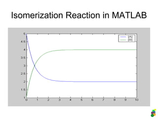
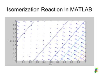
![Description in MATLAB:
2. Reversible Reaction
M-file (description of the model)
function dydt = isomerisation(t, y)
% A <-> B or y(1) <-> y(2)
k1 = 1;
k2 = 0.5;
dydt = [-k1*y(1)+k2*y(2) % d[A]/dt
k1*y(1)-k2*y(2) % d[B]/dt
];
Analysis of the model
>> [t y] = ode45(@isomerisation, [0 10], [5
1]);
>> plot (t, y);
>> legend ('[A]', '[B]');](https://image.slidesharecdn.com/mscitmodellingbiologicalsystems2005-150414002823-conversion-gate01/85/M-sc-it_modelling_biological_systems2005-22-320.jpg)

![Euler’s method in Perl
sub ode_euler {
my ($t0, $t_end, $h, $yref, $dydt_ref) = @_;
my @y = @$yref;
my @solution;
for (my $t = $t0; $t < $t_end; $t += $h) {
push @solution, [@y];
my @dydt = &$dydt_ref(@y, $t);
foreach my $i (0..$#y) {
$y[$i] += ( $h * $dydt[$i] );
}
}
push @solution, [@y];
return @solution;
}
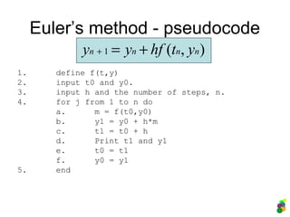
),(1 nnnn ythfyy +=+](https://image.slidesharecdn.com/mscitmodellingbiologicalsystems2005-150414002823-conversion-gate01/85/M-sc-it_modelling_biological_systems2005-26-320.jpg)
![Euler’s method in Perl
#!/usr/bin/perl -w
use strict;
my @initial_values = (5, 1);
my @result = ode_euler (0, 10, 0.01, @initial_values, &dydt);
foreach (@result) {
print join " ", @$_, "n";
}
exit;
% simple A <-> B reversible mono-molecular reaction
sub dydt {
my $yref = shift;
my @y = @$yref;
my @dydt = ( -$y[0] + 0.5*$y[1],
+$y[0] - 0.5*$y[1]
);
return @dydt;
}
....](https://image.slidesharecdn.com/mscitmodellingbiologicalsystems2005-150414002823-conversion-gate01/85/M-sc-it_modelling_biological_systems2005-27-320.jpg)


![Irreversible, two-molecule reaction
A+BC
Differential equations:
]][[
][
][][][
BAk
dt
Ad
dt
Cd
dt
Bd
dt
Ad
−=
−==
Underlying idea: Reaction probability = Combined probability that both
[A] and [B] are in a “reactive mood”:
]][[][][)()()( *
2
*
1 BAkBkAkBpApABp ===
The last piece of the puzzle
Non-linear!](https://image.slidesharecdn.com/mscitmodellingbiologicalsystems2005-150414002823-conversion-gate01/85/M-sc-it_modelling_biological_systems2005-31-320.jpg)
![A simple metabolic pathway
ABC+D
Differential equations:
d/dt decay forward reverse
[A]= -k1[A]
[B]= +k1[A] -k2[B] +k3[C][D]
[C]= +k2[B] -k3[C][D]
[D]= +k2[B] -k3[C][D]](https://image.slidesharecdn.com/mscitmodellingbiologicalsystems2005-150414002823-conversion-gate01/85/M-sc-it_modelling_biological_systems2005-32-320.jpg)
![Metabolic Networks as Bigraphs
ABC+D
d/dt decay forward reverse
[A] -k1[A]
[B] +k1[A] -k2[B] +k3[C][D]
[C] +k2[B] -k3[C][D]
[D] +k2[B] -k3[C][D]
k1 k2 k3
A -1 0 0
B 1 -1 1
C 0 1 -1
D 0 1 -1](https://image.slidesharecdn.com/mscitmodellingbiologicalsystems2005-150414002823-conversion-gate01/85/M-sc-it_modelling_biological_systems2005-33-320.jpg)


![Description in MATLAB:
3. The RKIP/ERK pathway
dydt = [
-k1*y(1)*y(2) + k2*y(3) + k5*y(4)
-k1*y(1)*y(2) + k2*y(3) + k11*y(11)
k1*y(1)*y(2) - k2*y(3) - k3*y(3)*y(9) + k4*y(4)
k3*y(3)*y(9) - k4*y(4) - k5*y(4)
k5*y(4) - k6*y(5)*y(7) + k7*y(8)
k5*y(4) - k9*y(6)*y(10) + k10*y(11)
-k6*y(5)*y(7) + k7*y(8) + k8*y(8)
k6*y(5)*y(7) - k7*y(8) - k8*y(8)
-k3*y(3)*y(9) + k4*y(4) + k8*y(8)
-k9*y(6)*y(10) + k10*y(11) + k11*y(11)
k9*y(6)*y(10) - k10*y(11) - k11*y(11)
];](https://image.slidesharecdn.com/mscitmodellingbiologicalsystems2005-150414002823-conversion-gate01/85/M-sc-it_modelling_biological_systems2005-43-320.jpg)
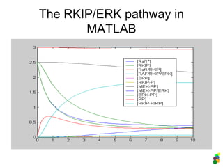
![Description in MATLAB:
3. The RKIP/ERK pathway
Analysis of the model:
>> [t y] =
ode45(@erk_pathway_wolkenhauer, [0
10], [2.5 2.5 0 0 0 0 2.5 0 2.5 3
0]); %(initial values!)
>> plot (t, y);
>> legend ('[Raf1*]', '[RKIP]',
'[Raf1/RKIP]', '[RAF/RKIP/ERK]',
'[ERK]', '[RKIP-P]', '[MEK-PP]',
'[MEK-PP/ERK]', '[ERK-PP]', '[RP]',
'[RKIP-P/RP]' );](https://image.slidesharecdn.com/mscitmodellingbiologicalsystems2005-150414002823-conversion-gate01/85/M-sc-it_modelling_biological_systems2005-44-320.jpg)

![Example of Sensitivity Analysis
function [tt,yy] = sensitivity(f, range, initvec,
which_stuff_vary, ep, step, which_stuff_show,
timeres);
timevec = range(1):timeres:range(2);
vec = [initvec];
[tt y] = ode45(f, timevec, vec);
yy = y(:,which_stuff_show);
for i=initvec(which_stuff_vary)+step:step:ep;
vec(which_stuff_vary) = i;
[t y] = ode45(f, timevec, vec);
tt = [t];
yy = [yy y(:,which_stuff_show)];
end](https://image.slidesharecdn.com/mscitmodellingbiologicalsystems2005-150414002823-conversion-gate01/85/M-sc-it_modelling_biological_systems2005-47-320.jpg)
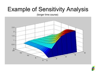
![Example of Sensitivity Analysis
>> [t y] =
sensitivity(@erk_pathway_wolken
hauer, [0 1], [2.5 2.5 0 0 0 0
2.5 0 2.5 3 0], 5, 6, 1, 8,
0.05);
>> surf (y);
varies concentration of m5 (ERK-PP) from
0..6, outputs concentration of m8
(ERK/MEK-PP), time range [0 1], steps of
0.05. Then plots a surface map.](https://image.slidesharecdn.com/mscitmodellingbiologicalsystems2005-150414002823-conversion-gate01/85/M-sc-it_modelling_biological_systems2005-48-320.jpg)


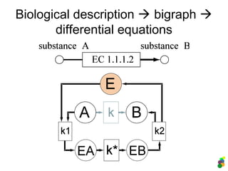
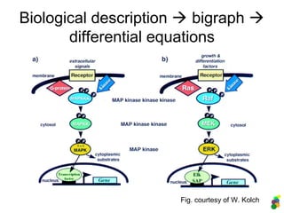
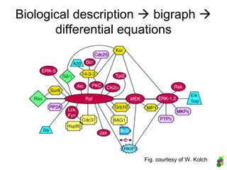
This document discusses modelling biological systems using differential equations. It begins by outlining why modelling is important given that biological systems contain dozens of interacting components in nonlinear ways. It then covers the statistical physics behind modelling, showing how simple chemical reactions can be described by ordinary differential equations. It provides examples of modelling kinetics, probabilities, and spatial heterogeneity. Finally, it demonstrates how to translate a biological description into a mathematical model using differential equations, providing the example of the Raf-1/RKIP/ERK pathway.


![11.[8 17]numerical solution of fuzzy hybrid differential equation by third or...](https://cdn.slidesharecdn.com/ss_thumbnails/11-8-17numericalsolutionoffuzzyhybriddifferentialequationbythirdorderrungekuttanystrommethod-120512235447-phpapp02-thumbnail.jpg?width=640&height=640&fit=bounds)