The document summarizes techniques for solving linear systems of equations. It discusses direct solution methods like Gaussian elimination that transform the system into an upper triangular system and then use back substitution to solve. Gaussian elimination involves using elementary row operations to eliminate values below the diagonal of the coefficient matrix. The document also discusses concepts like consistency, uniqueness of solutions, and ill-conditioned systems. It provides examples of applying elementary row operations during the Gaussian elimination process.
1
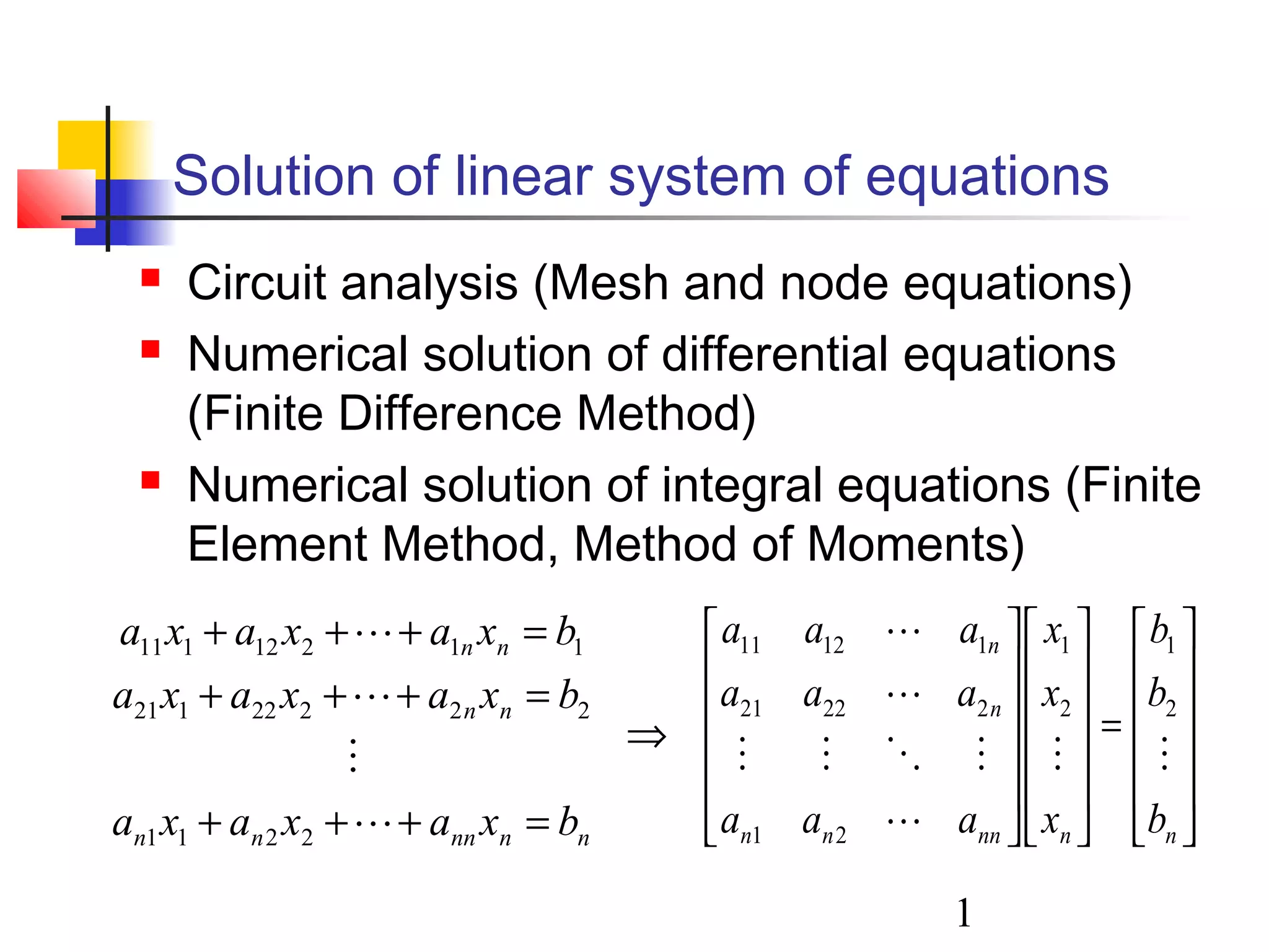
Solution of linearsystem of equations
Circuit analysis (Mesh and node equations)
Numerical solution of differential equations
(Finite Difference Method)
Numerical solution of integral equations (Finite
Element Method, Method of Moments)
nnnnnn
nn
nn
bxaxaxa
bxaxaxa
bxaxaxa
=+++
=+++
=+++
2211
22222121
11212111
=
nnnnnn
n
n
b
b
b
x
x
x
aaa
aaa
aaa
2
1
2
1
21
22221
11211
⇒
2.
2
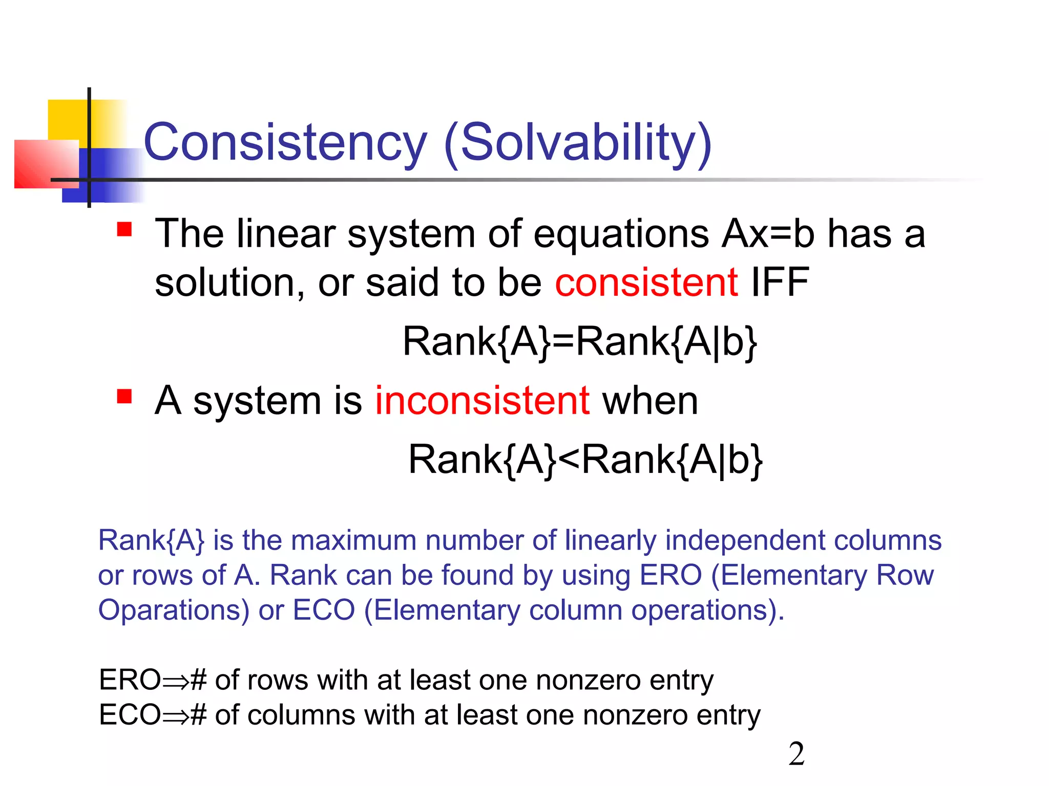
Consistency (Solvability)
Thelinear system of equations Ax=b has a
solution, or said to be consistent IFF
Rank{A}=Rank{A|b}
A system is inconsistent when
Rank{A}<Rank{A|b}
Rank{A} is the maximum number of linearly independent columns
or rows of A. Rank can be found by using ERO (Elementary Row
Oparations) or ECO (Elementary column operations).
ERO⇒# of rows with at least one nonzero entry
ECO⇒# of columns with at least one nonzero entry
3.
3
Elementary row operations
The following operations applied to the
augmented matrix [A|b], yield an equivalent
linear system
Interchanges: The order of two rows can be
changed
Scaling: Multiplying a row by a nonzero constant
Replacement: The row can be replaced by the sum
of that row and a nonzero multiple of any other row.
5
Uniqueness of solutions
The system has a unique solution IFF
Rank{A}=Rank{A|b}=n
n is the order of the system
Such systems are called full-rank systems
6.
6
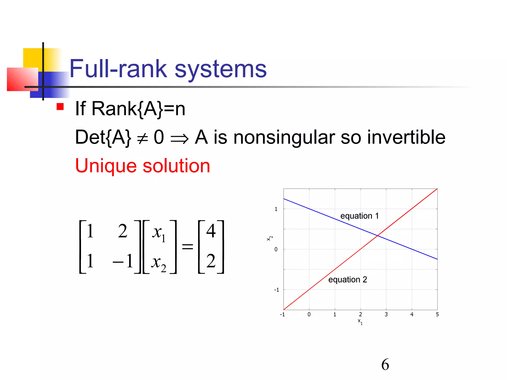
Full-rank systems
IfRank{A}=n
Det{A} ≠ 0 ⇒ A is nonsingular so invertible
Unique solution
=
− 2
4
11
21
2
1
x
x
7.
7
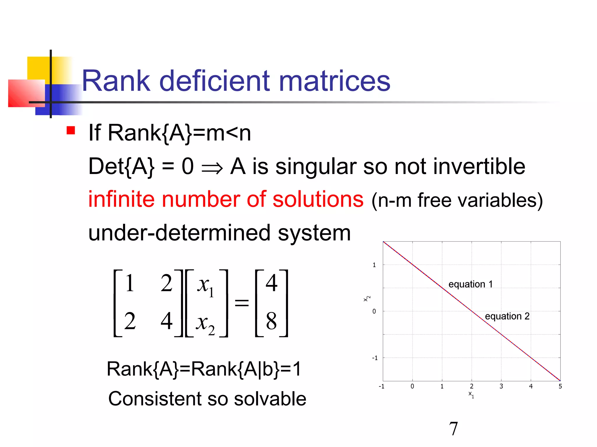
Rank deficient matrices
If Rank{A}=m<n
Det{A} = 0 ⇒ A is singular so not invertible
infinite number of solutions (n-m free variables)
under-determined system
=
8
4
42
21
2
1
x
x
Consistent so solvable
Rank{A}=Rank{A|b}=1
8.
8
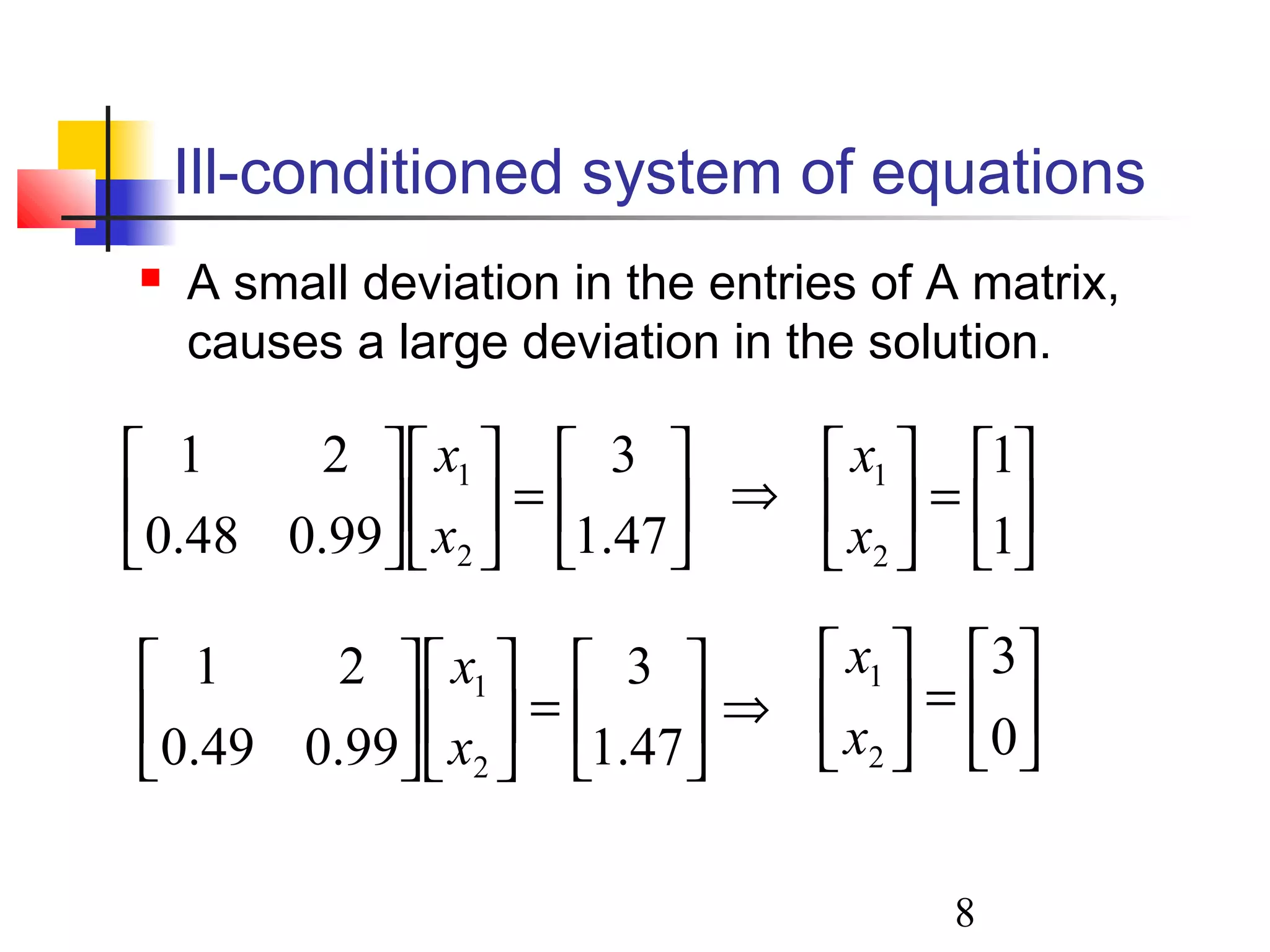
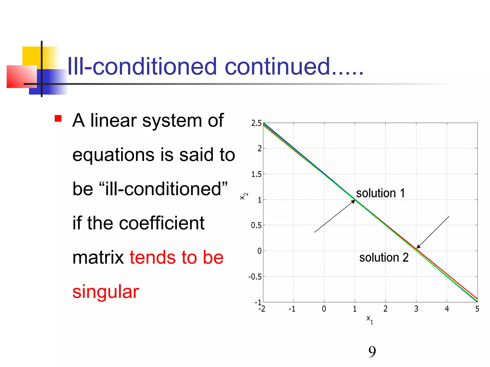
Ill-conditioned system ofequations
A small deviation in the entries of A matrix,
causes a large deviation in the solution.
=
47.1
3
99.048.0
21
2
1
x
x
=
47.1
3
99.049.0
21
2
1
x
x
=
1
1
2
1
x
x
⇒
=
0
3
2
1
x
x
⇒
10
Types of linearsystem of equations to be
studied in this course
Coefficient matrix A is square and real
The RHS vector b is nonzero and real
Consistent system, solvable
Full-rank system, unique solution
Well-conditioned system
11.
11
Solution Techniques
Directsolution methods
Finds a solution in a finite number of operations by
transforming the system into an equivalent system
that is ‘easier’ to solve.
Diagonal, upper or lower triangular systems are
easier to solve
Number of operations is a function of system size n.
Iterative solution methods
Computes succesive approximations of the solution
vector for a given A and b, starting from an initial
point x0.
Total number of operations is uncertain, may not
converge.
12.
12
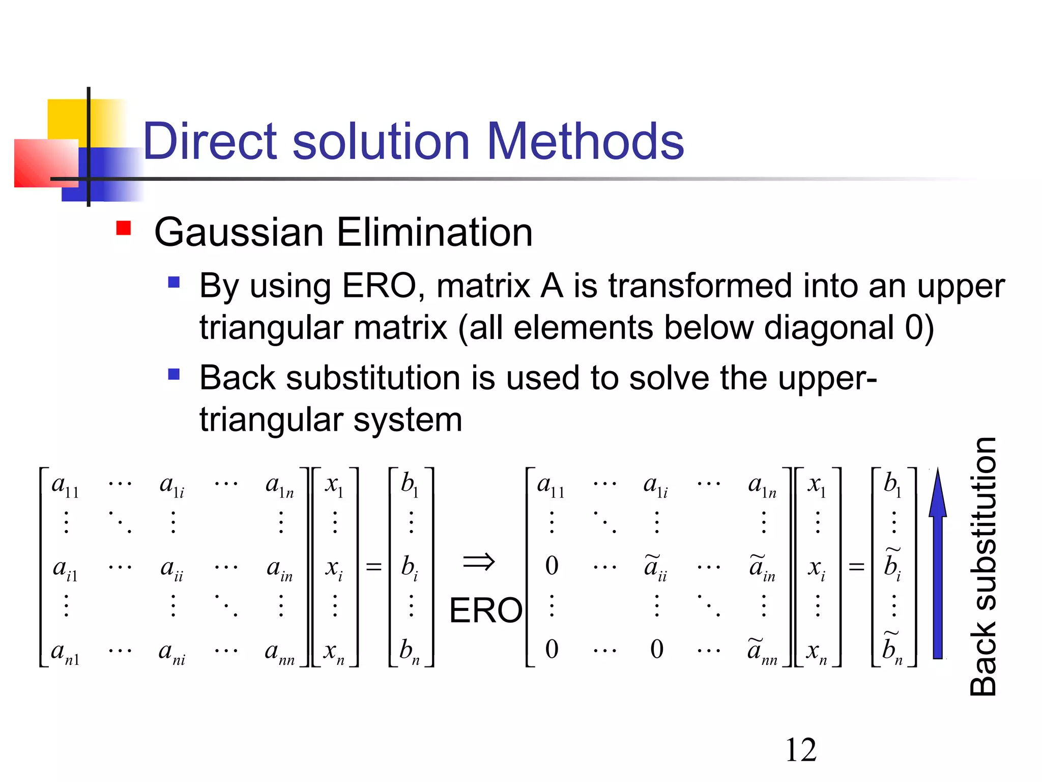
Direct solution Methods
Gaussian Elimination
By using ERO, matrix A is transformed into an upper
triangular matrix (all elements below diagonal 0)
Back substitution is used to solve the upper-
triangular system
=
n
i
n
i
nnnin
iniii
ni
b
b
b
x
x
x
aaa
aaa
aaa
11
1
1
1111
⇒
ERO
=
n
i
n
i
nn
inii
ni
b
b
b
x
x
x
a
aa
aaa
~
~
~00
~~0
111111
Backsubstitution
13.
13
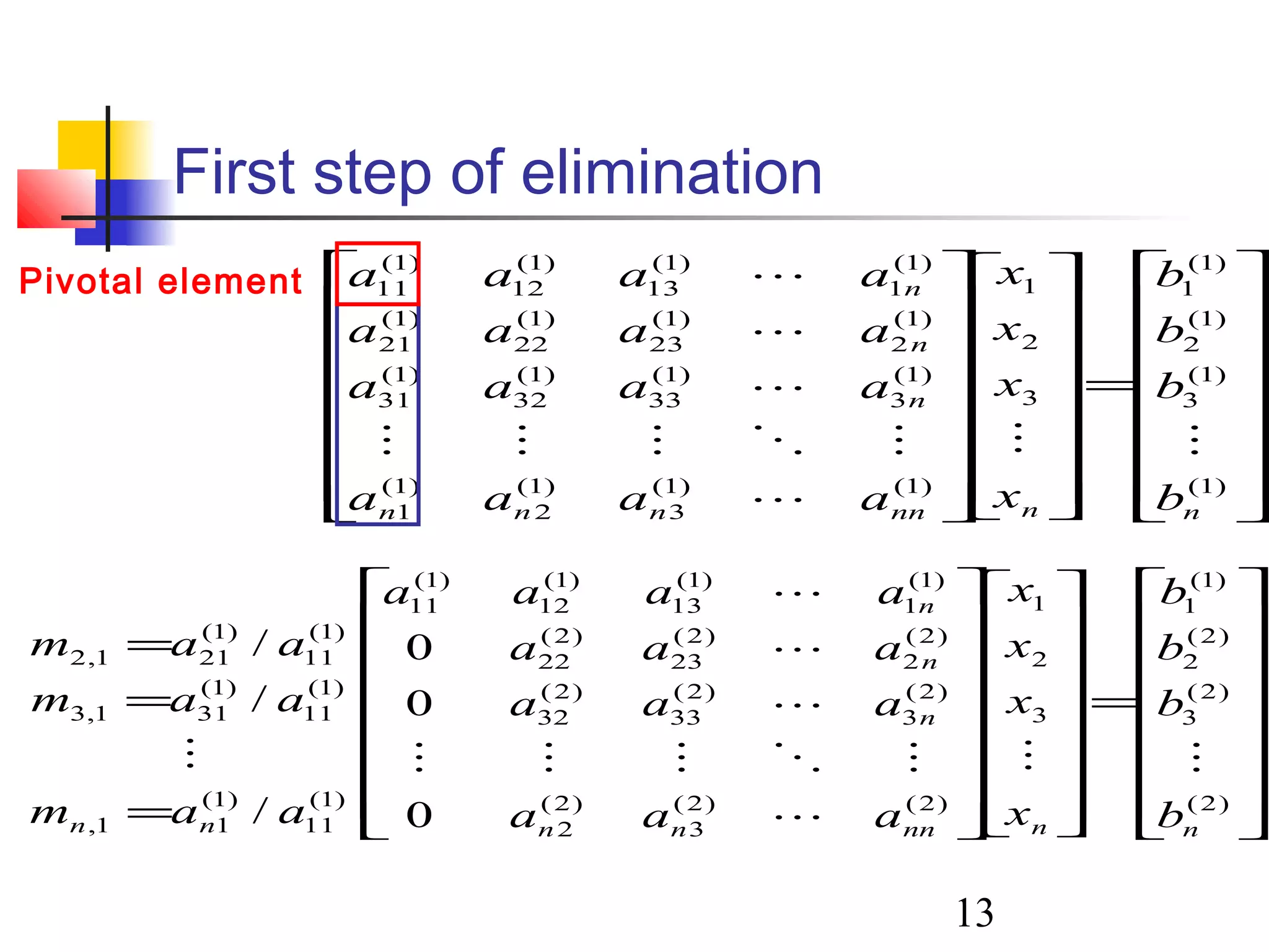
First step ofelimination
=
=
=
=
)2(
)2(
3
)2(
2
)1(
1
3
2
1
)2()2(
3
)2(
2
)2(
3
)2(
33
)2(
32
)2(
2
)2(
23
)2(
22
)1(
1
)1(
13
)1(
12
)1(
11
)1(
11
)1(
11,
)1(
11
)1(
311,3
)1(
11
)1(
211,2
0
0
0
/
/
/
nnnnnn
n
n
n
nn b
b
b
b
x
x
x
x
aaa
aaa
aaa
aaaa
aam
aam
aam
=
)1(
)1(
3
)1(
2
)1(
1
3
2
1
)1()1(
3
)1(
2
)1(
1
)1(
3
)1(
33
)1(
32
)1(
31
)1(
2
)1(
23
)1(
22
)1(
21
)1(
1
)1(
13
)1(
12
)1(
11
nnnnnnn
n
n
n
b
b
b
b
x
x
x
x
aaaa
aaaa
aaaa
aaaa
Pivotal element
14.
14
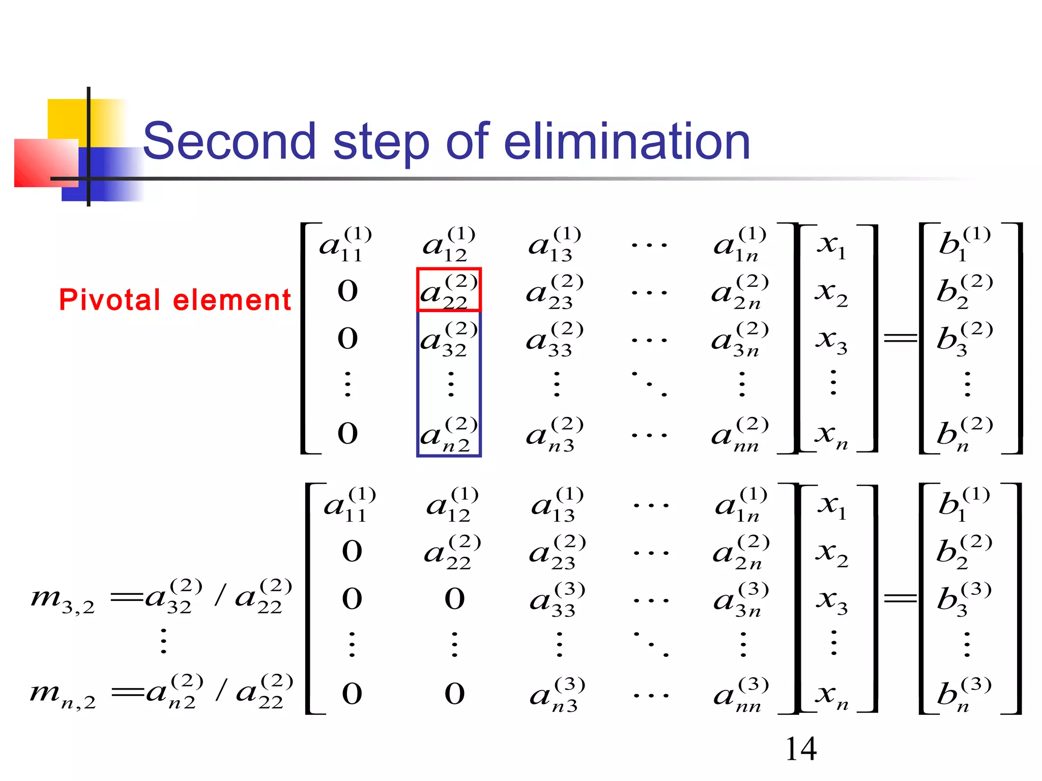
Second step ofelimination
=
=
=
)3(
)3(
3
)2(
2
)1(
1
3
2
1
)3()3(
3
)3(
3
)3(
33
)2(
2
)2(
23
)2(
22
)1(
1
)1(
13
)1(
12
)1(
11
)2(
22
)2(
22,
)2(
22
)2(
322,3
00
00
0
/
/
nnnnn
n
n
n
nn b
b
b
b
x
x
x
x
aa
aa
aaa
aaaa
aam
aam
=
)2(
)2(
3
)2(
2
)1(
1
3
2
1
)2()2(
3
)2(
2
)2(
3
)2(
33
)2(
32
)2(
2
)2(
23
)2(
22
)1(
1
)1(
13
)1(
12
)1(
11
0
0
0
nnnnnn
n
n
n
b
b
b
b
x
x
x
x
aaa
aaa
aaa
aaaa
Pivotal element
15.
15
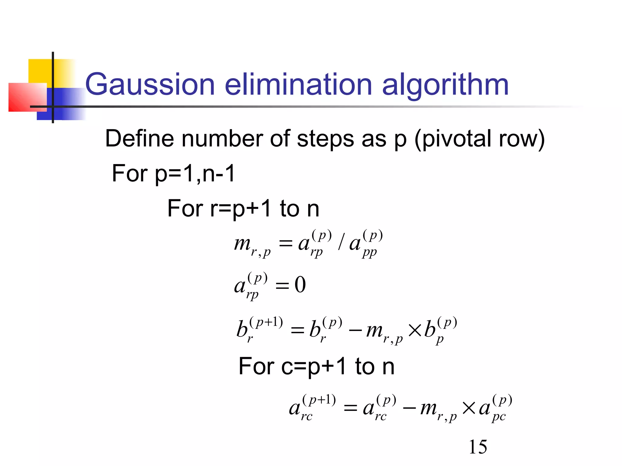
Gaussion elimination algorithm
Definenumber of steps as p (pivotal row)
For p=1,n-1
For r=p+1 to n
For c=p+1 to n
0
/
)(
)()(
,
=
=
p
rp
p
pp
p
rppr
a
aam
)(
,
)()1( p
pcpr
p
rc
p
rc amaa ×−=+
)(
,
)()1( p
ppr
p
r
p
r bmbb ×−=+
17
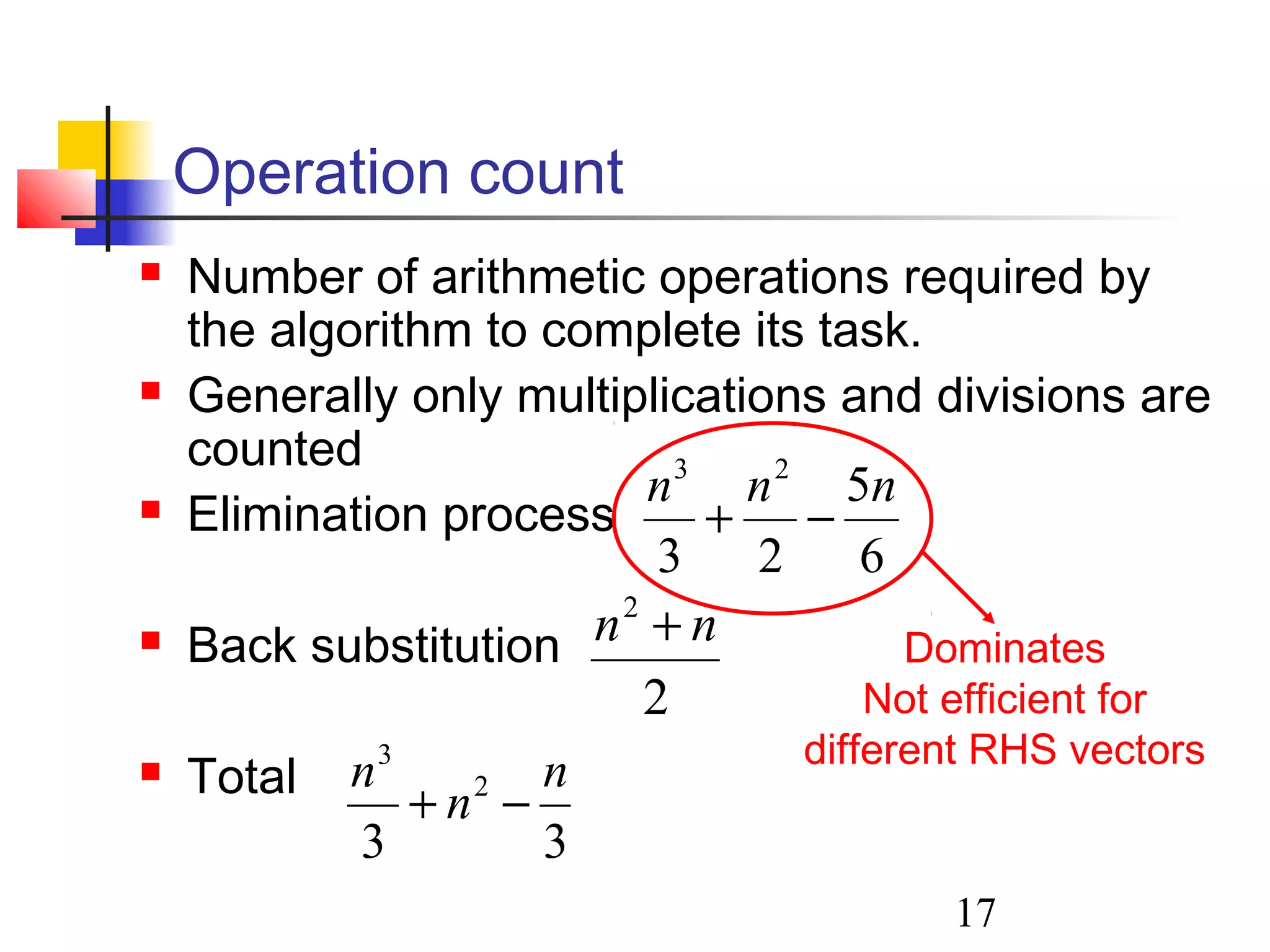
Operation count
Numberof arithmetic operations required by
the algorithm to complete its task.
Generally only multiplications and divisions are
counted
Elimination process
Back substitution
Total
6
5
23
23
nnn
−+
2
2
nn +
33
2
3
n
n
n
−+
Dominates
Not efficient for
different RHS vectors
18.
18
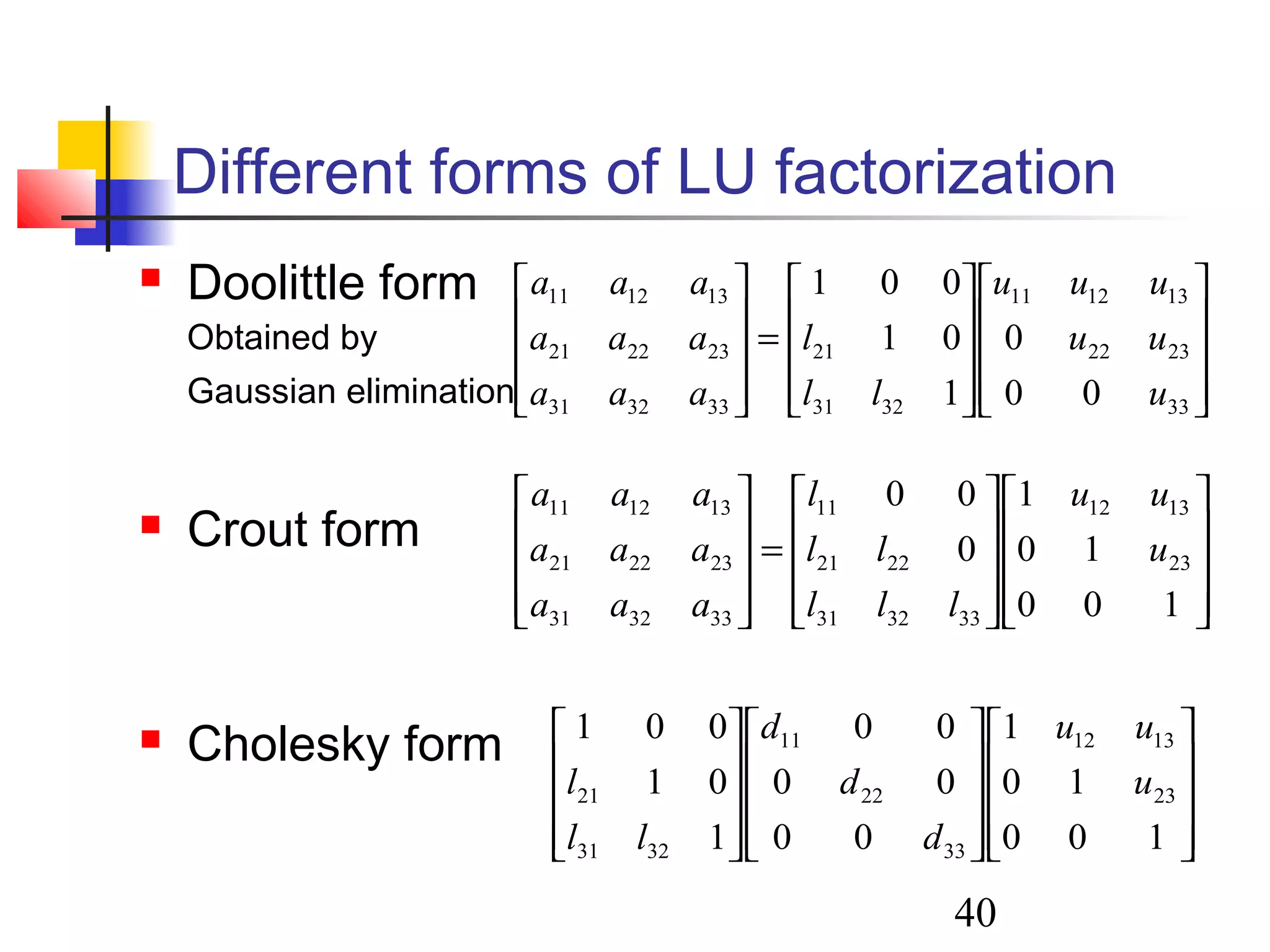
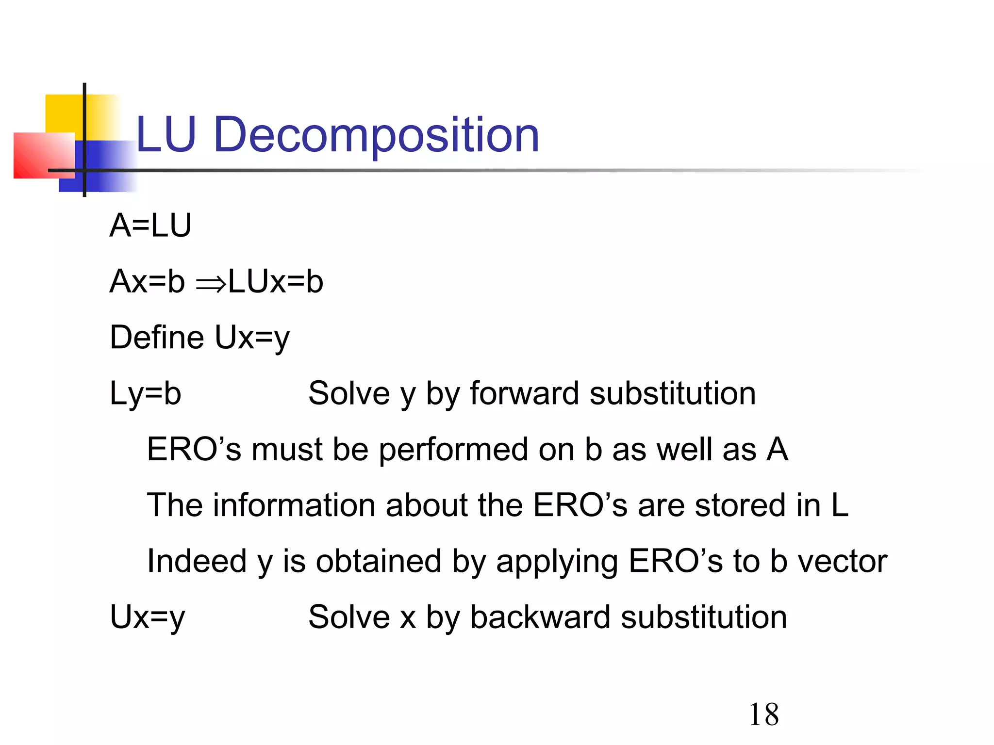
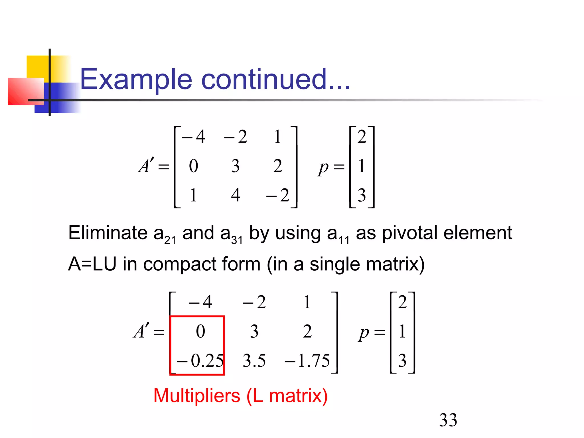
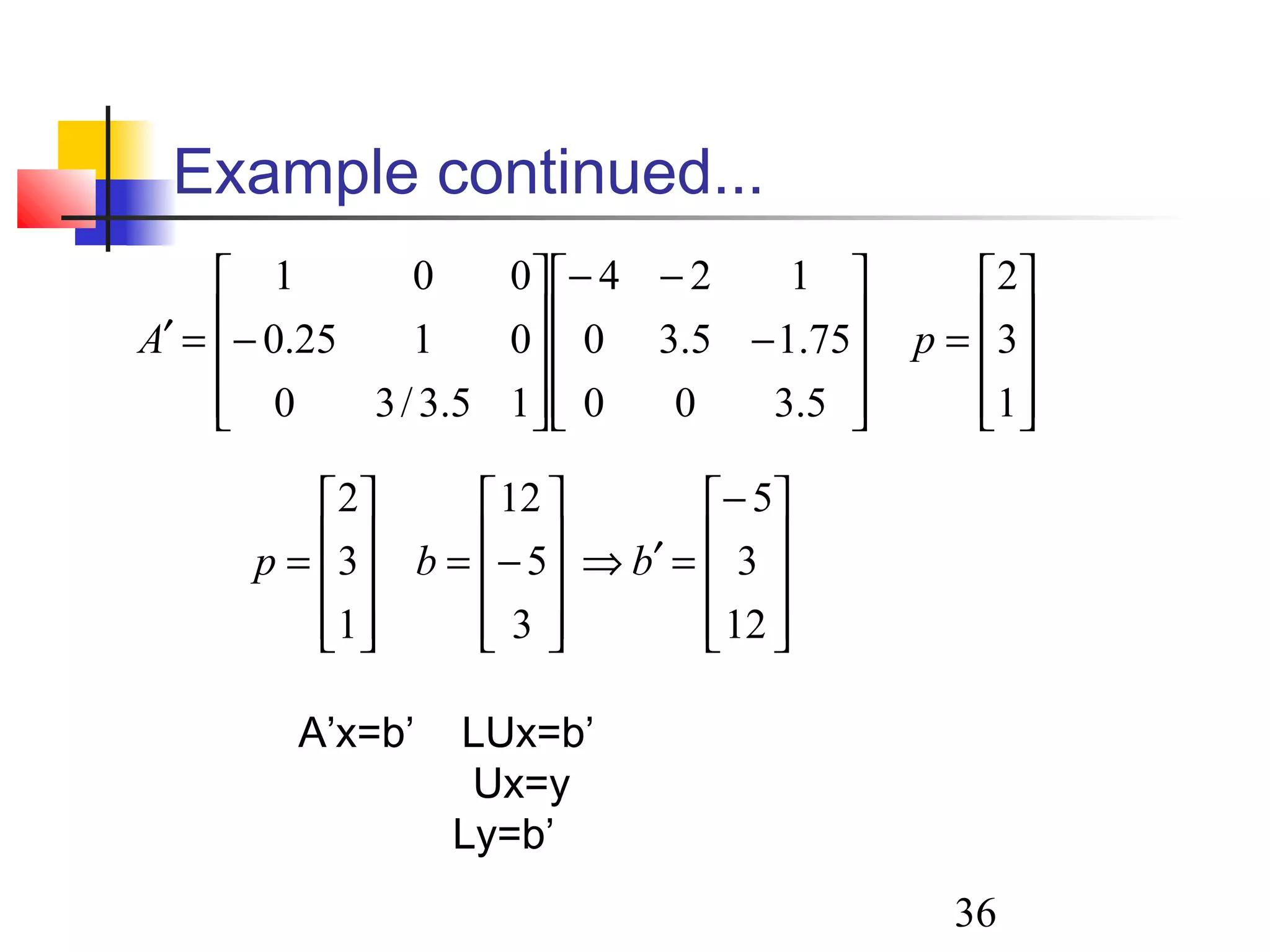
LU Decomposition
A=LU
Ax=b ⇒LUx=b
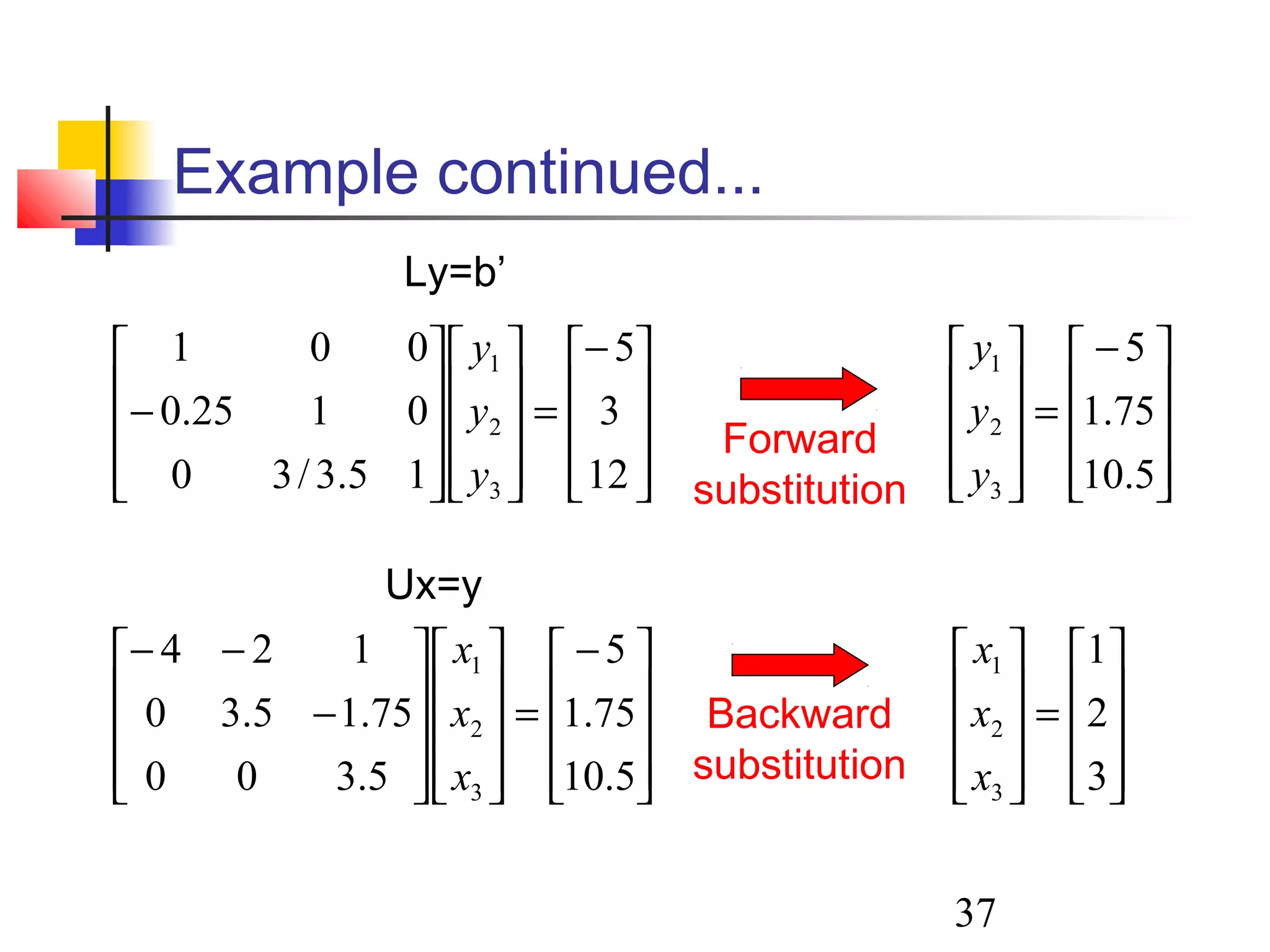
DefineUx=y
Ly=b Solve y by forward substitution
ERO’s must be performed on b as well as A
The information about the ERO’s are stored in L
Indeed y is obtained by applying ERO’s to b vector
Ux=y Solve x by backward substitution
19.
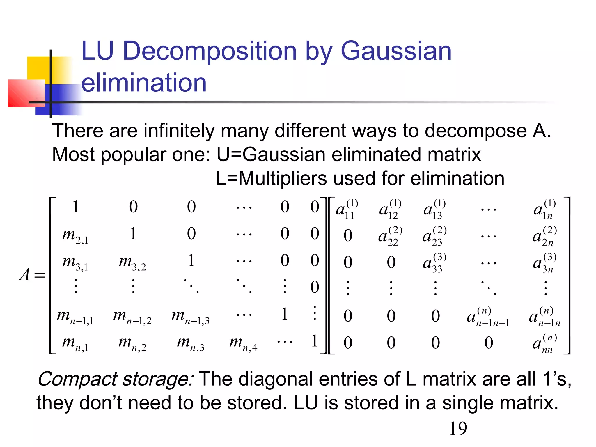
19
LU Decomposition byGaussian
elimination
=
−−−−−−
)(
)(
1
)(
11
)3(
3
)3(
33
)2(
2
)2(
23
)2(
22
)1(
1
)1(
13
)1(
12
)1(
11
4,3,2,1,
3,12,11,1
2,31,3
1,2
0000
000
00
0
1
1
0
001
0001
00001
n
nn
n
nn
n
nn
n
n
n
nnnn
nnn
a
aa
aa
aaa
aaaa
mmmm
mmm
mm
m
A
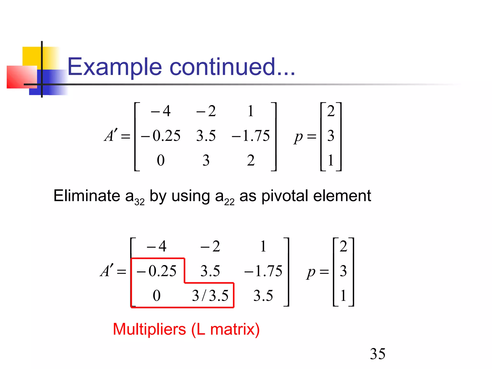
Compact storage: The diagonal entries of L matrix are all 1’s,
they don’t need to be stored. LU is stored in a single matrix.
There are infinitely many different ways to decompose A.
Most popular one: U=Gaussian eliminated matrix
L=Multipliers used for elimination
20.
20
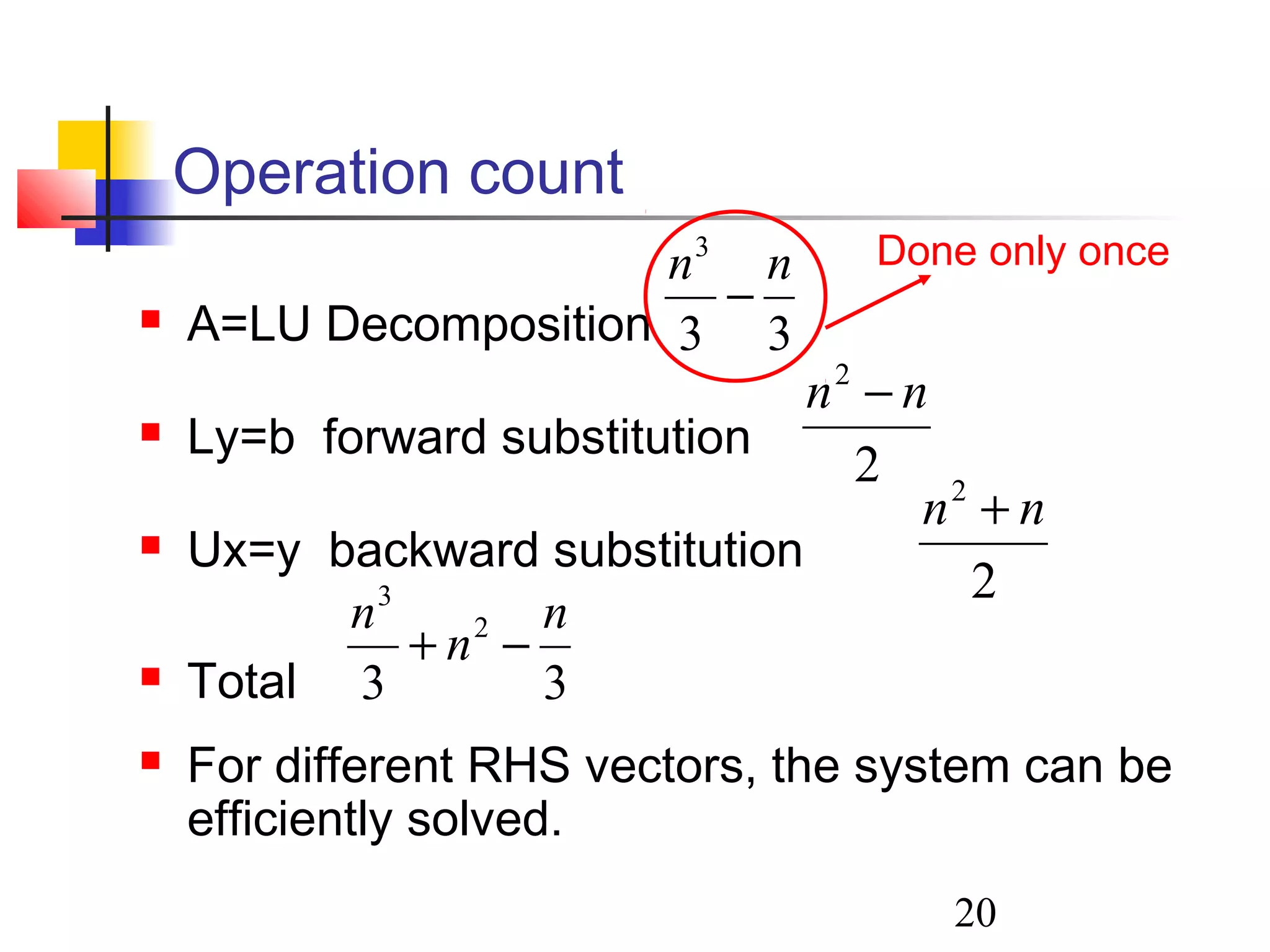
Operation count
A=LUDecomposition
Ly=b forward substitution
Ux=y backward substitution
Total
For different RHS vectors, the system can be
efficiently solved.
33
3
nn
−
2
2
nn +
2
2
nn −
33
2
3
n
n
n
−+
Done only once
21.
21
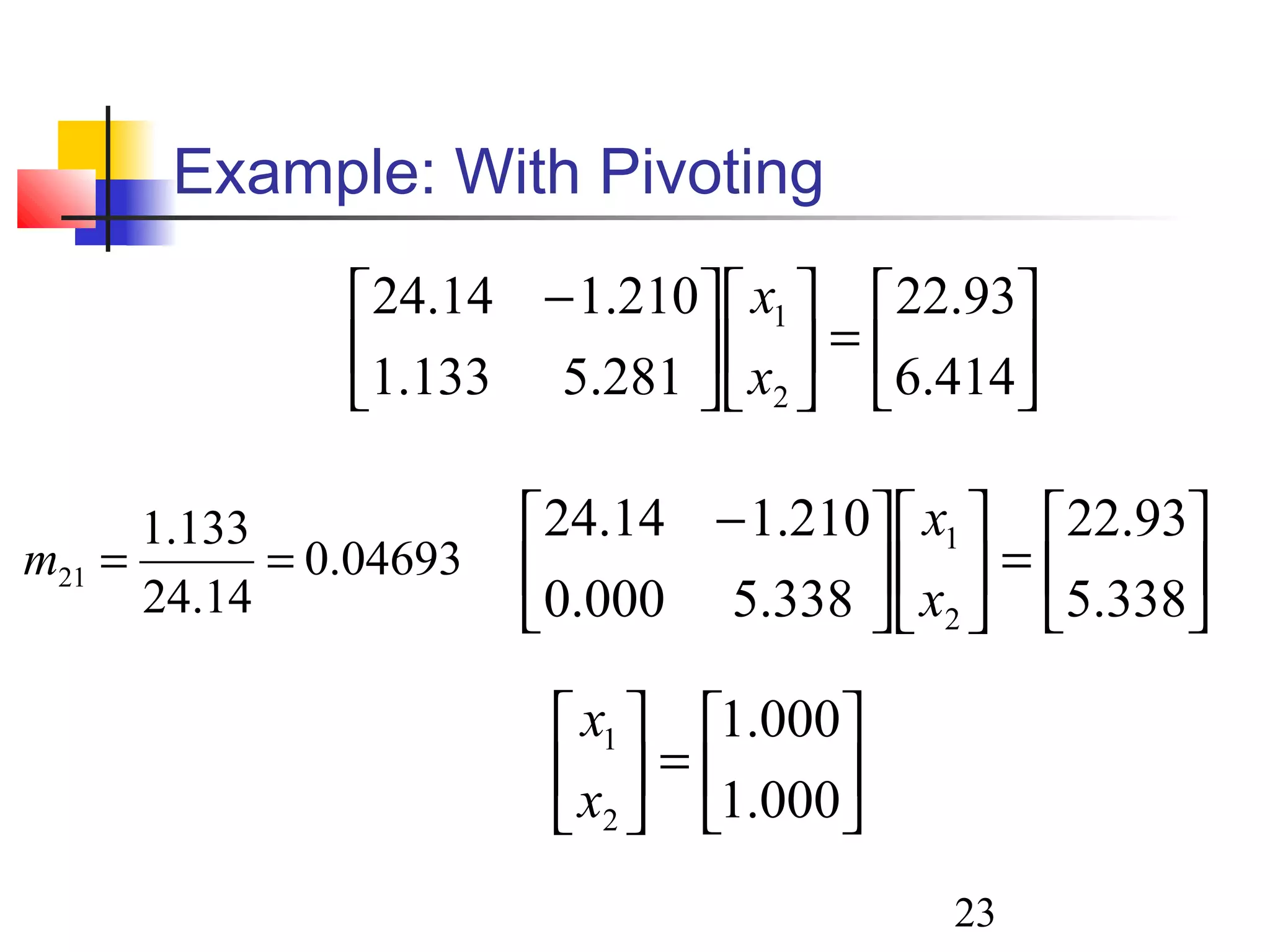
Pivoting
Computer usesfinite-precision arithmetic
A small error is introduced in each arithmetic
operation, error propagates
When the pivotal element is very small, the
multipliers will be large.
Adding numbers of widely differening
magnitude can lead to loss of significance.
To reduce error, row interchanges are made to
maximise the magnitude of the pivotal element
22.
22
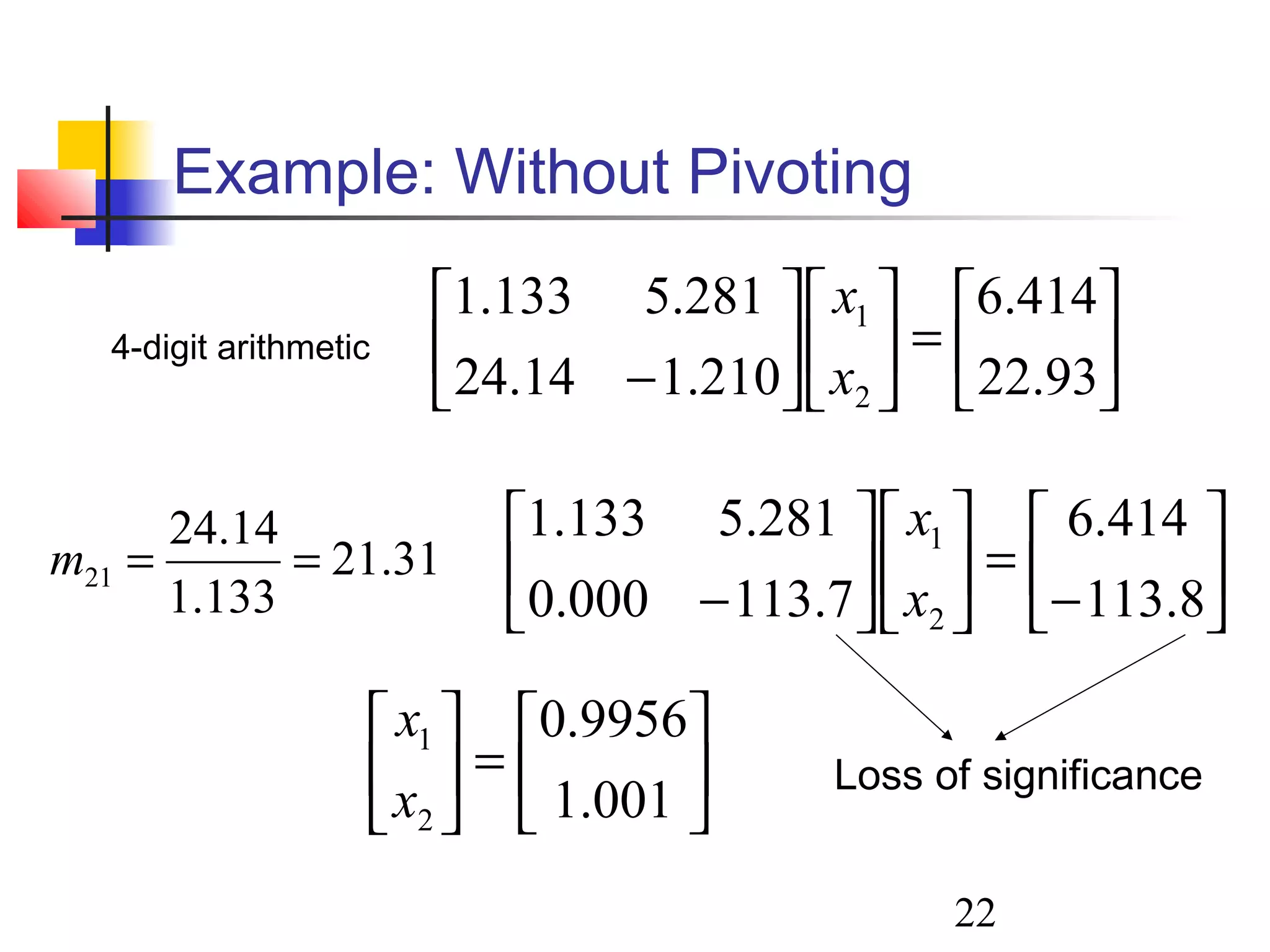
Example: Without Pivoting
=
−93.22
414.6
210.114.24
281.5133.1
2
1
x
x
−
=
− 8.113
414.6
7.113000.0
281.5133.1
2
1
x
x
=
001.1
9956.0
2
1
x
x
31.21
133.1
14.24
21 ==m
4-digit arithmetic
Loss of significance
25
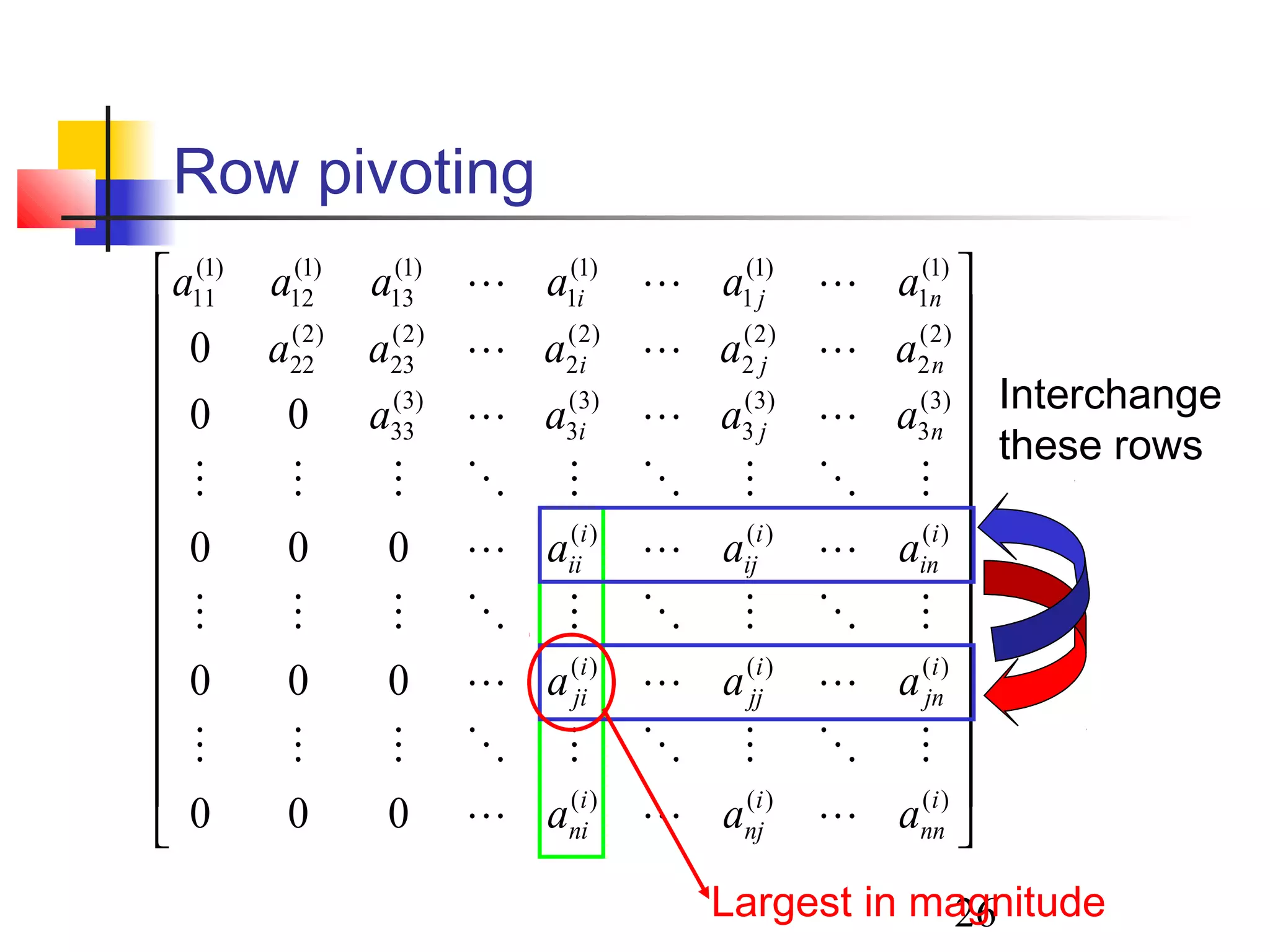
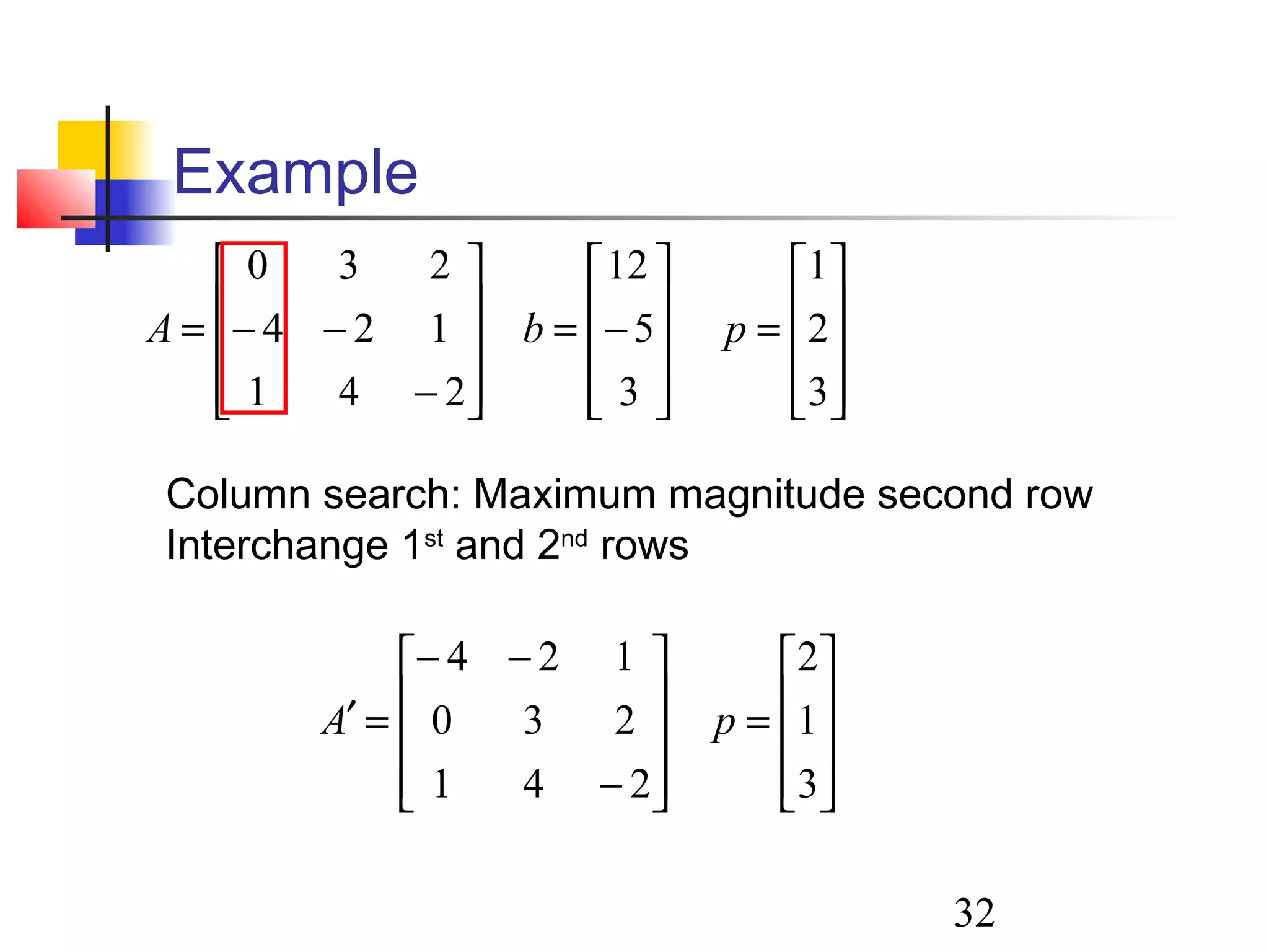
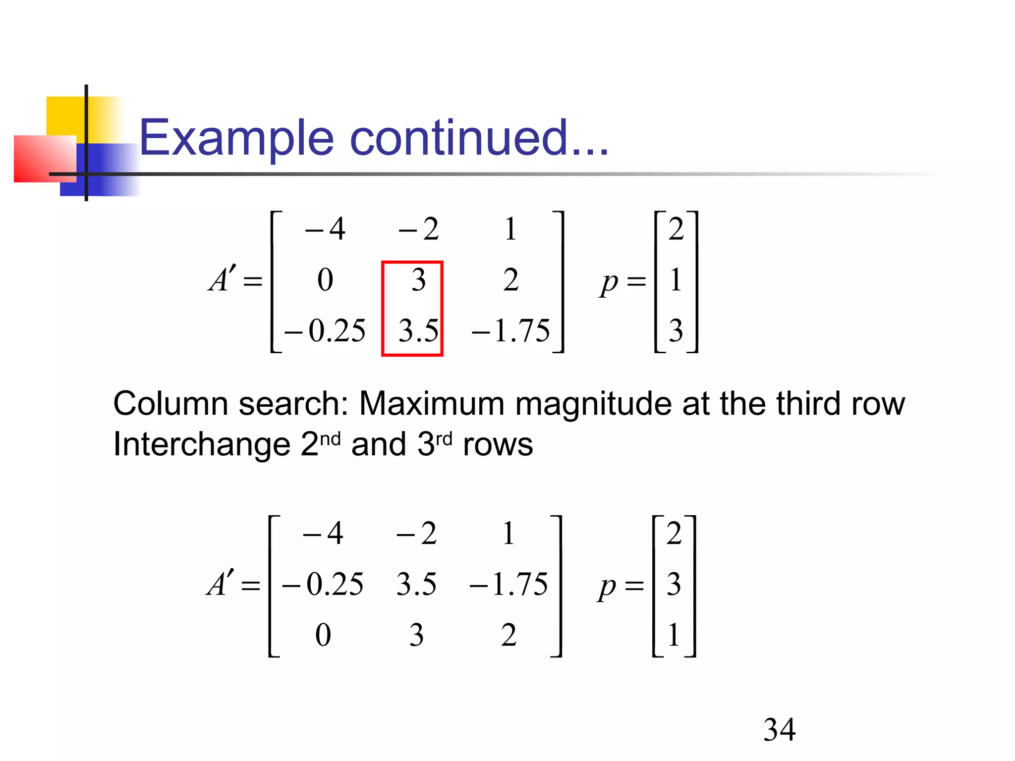
Row pivoting
Mostcommonly used partial pivoting procedure
Search the pivotal column
Find the largest element in magnitude
Then switch this row with the pivotal row
29
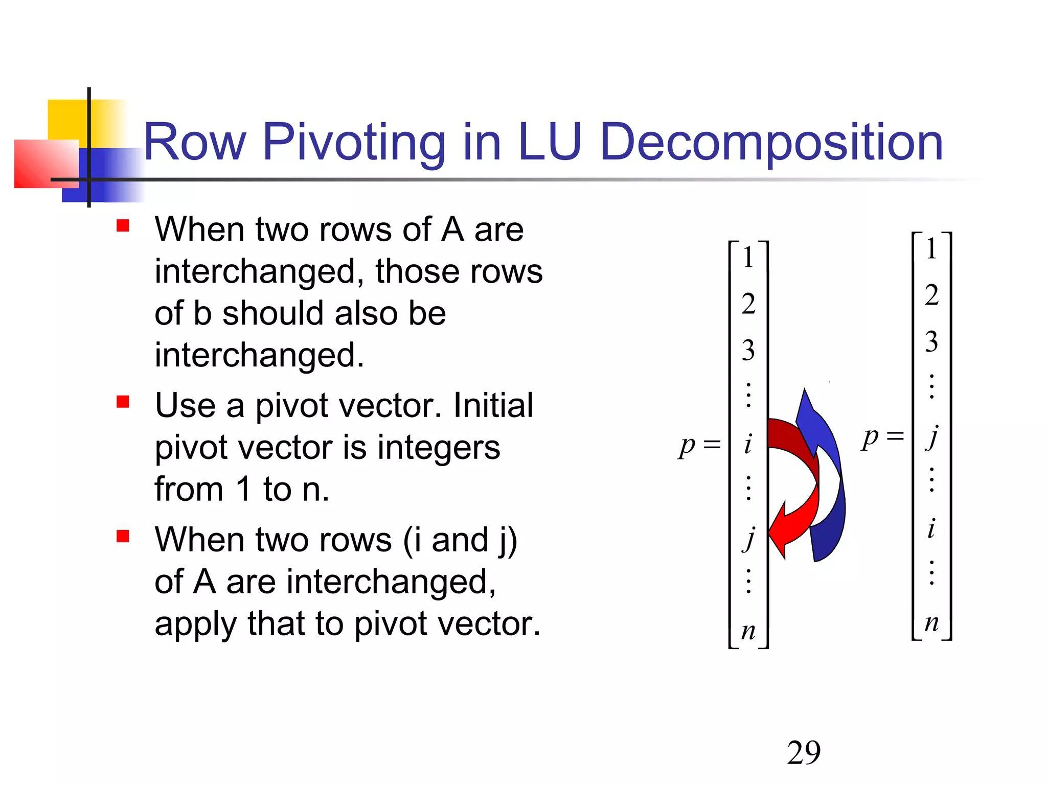
Row Pivoting inLU Decomposition
When two rows of A are
interchanged, those rows
of b should also be
interchanged.
Use a pivot vector. Initial
pivot vector is integers
from 1 to n.
When two rows (i and j)
of A are interchanged,
apply that to pivot vector.
=
n
i
jp
3
2
1
=
n
j
ip
3
2
1
30.
30
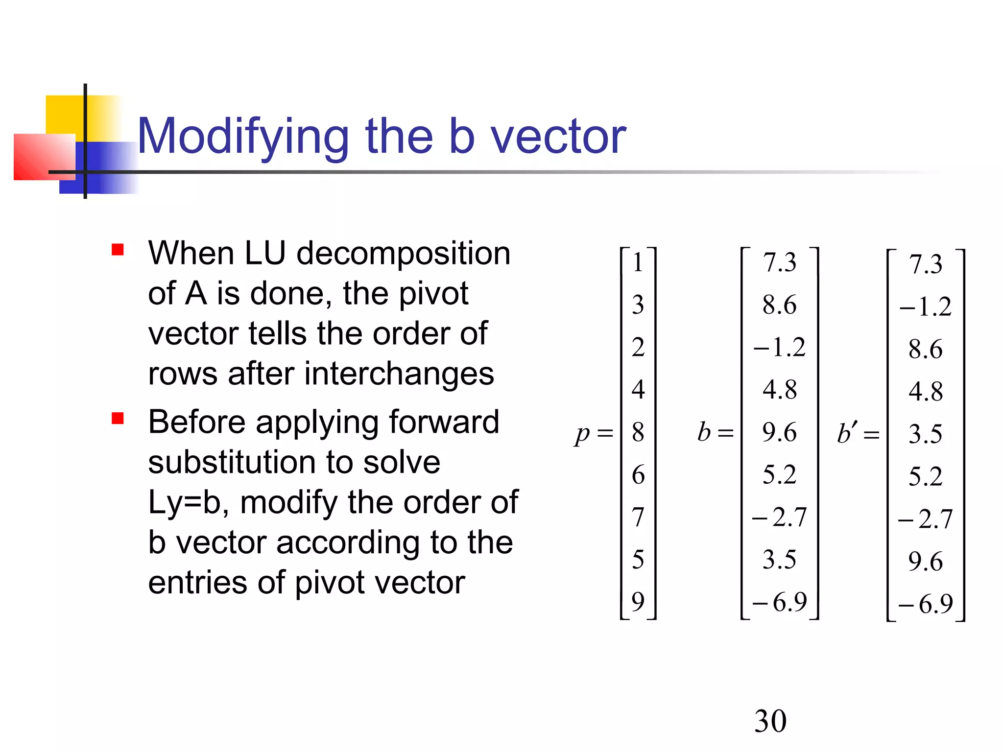
Modifying the bvector
When LU decomposition
of A is done, the pivot
vector tells the order of
rows after interchanges
Before applying forward
substitution to solve
Ly=b, modify the order of
b vector according to the
entries of pivot vector
=
9
5
7
6
8
4
2
3
1
p
−
−
−
=
9.6
5.3
7.2
2.5
6.9
8.4
2.1
6.8
3.7
b
−
−
−
=′
9.6
6.9
7.2
2.5
5.3
8.4
6.8
2.1
3.7
b
31.
31
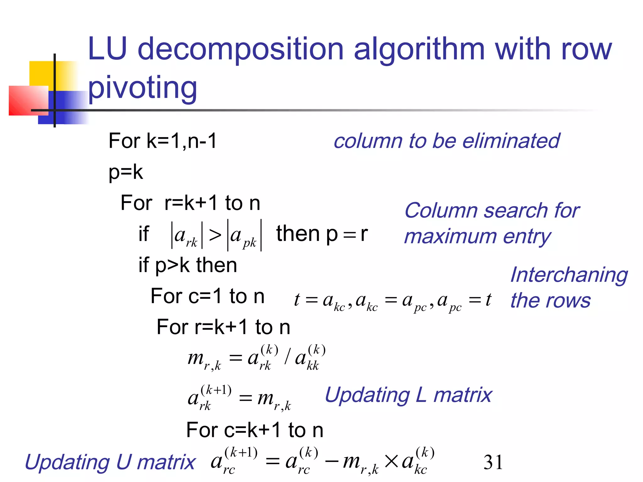
LU decomposition algorithmwith row
pivoting
For k=1,n-1 column to be eliminated
p=k
For r=k+1 to n
if
if p>k then
For c=1 to n
For r=k+1 to n
For c=k+1 to n
kr
k
rk
k
kk
k
rkkr
ma
aam
,
)1(
)()(
, /
=
=
+
)(
,
)()1( k
kckr
k
rc
k
rc amaa ×−=+
rpthen => pkrk aa
taaaat pcpckckc === ,,
Column search for
maximum entry
Interchaning
the rows
Updating L matrix
Updating U matrix
38
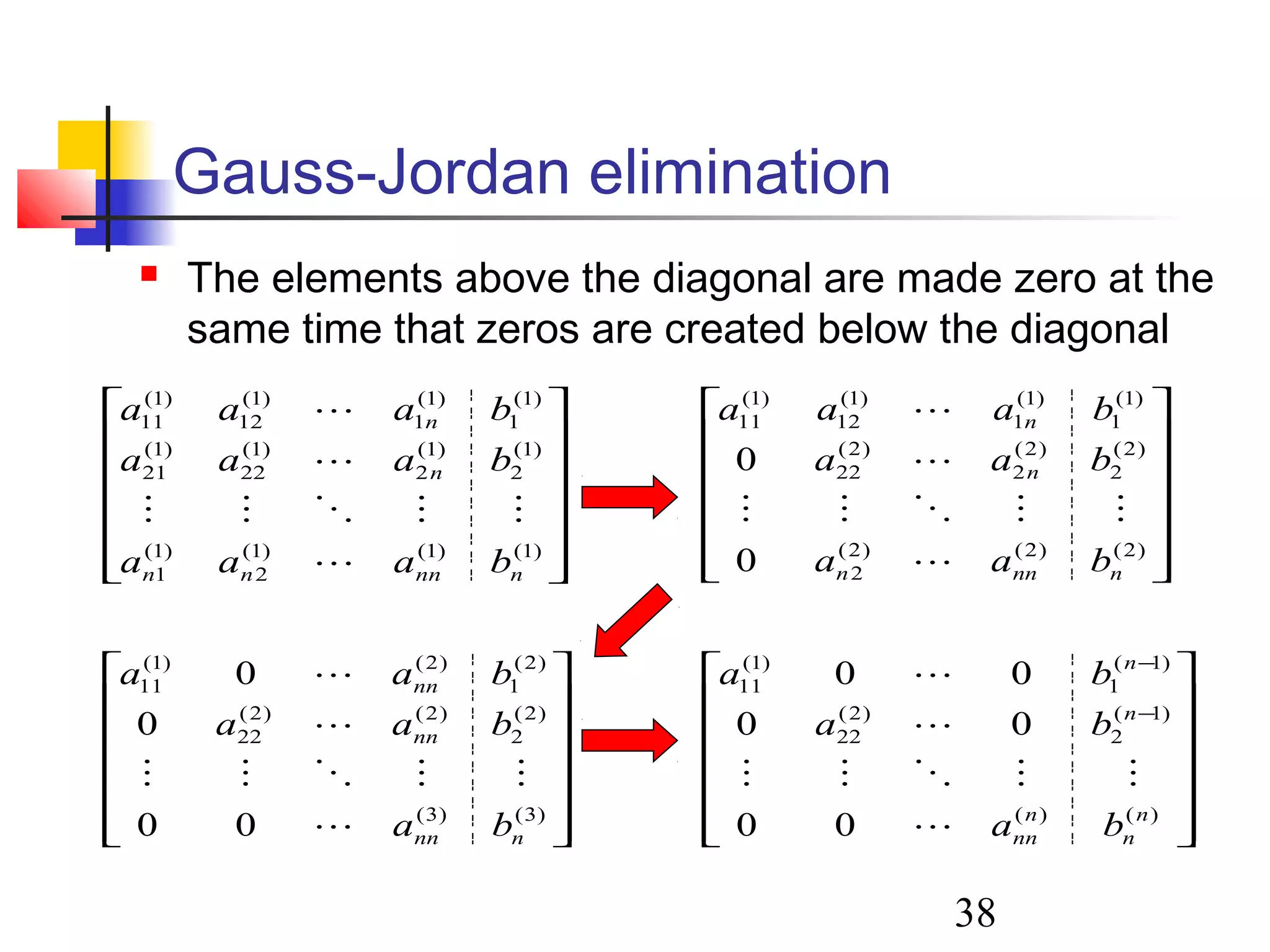
Gauss-Jordan elimination
Theelements above the diagonal are made zero at the
same time that zeros are created below the diagonal
)1()1()1(
2
)1(
1
)1(
2
)1(
2
)1(
22
)1(
21
)1(
1
)1(
1
)1(
12
)1(
11
nnnnn
n
n
baaa
baaa
baaa
)2()2()2(
2
)2(
2
)2(
2
)2(
22
)1(
1
)1(
1
)1(
12
)1(
11
0
0
nnnn
n
n
baa
baa
baaa
−
−
)()(
)1(
2
)2(
22
)1(
1
)1(
11
00
00
00
n
n
n
nn
n
n
ba
ba
ba
)3()3(
)2(
2
)2()2(
22
)2(
1
)2()1(
11
00
0
0
nnn
nn
nn
ba
baa
baa
39.
39
Gauss-Jordan Elimination
Almost50% more arithmetic operations than
Gaussian elimination
Gauss-Jordan (GJ) Elimination is prefered
when the inverse of a matrix is required.
Apply GJ elimination to convert A into an
identity matrix.
[ ]IA
[ ]1−
AI
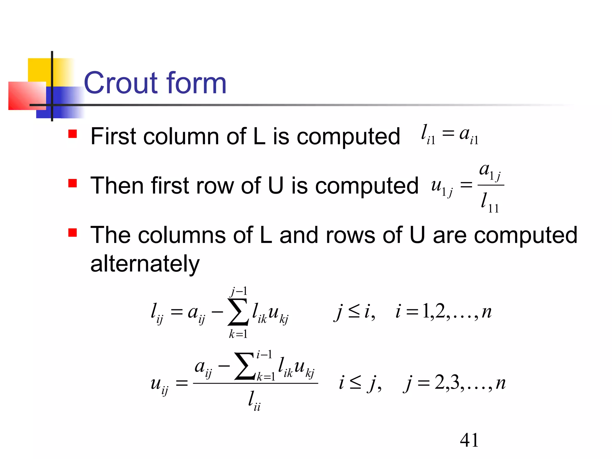
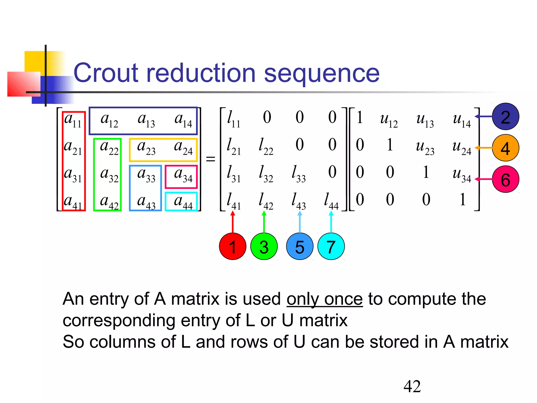
41
Crout form
Firstcolumn of L is computed
Then first row of U is computed
The columns of L and rows of U are computed
alternately
11 ii al =
11
1
1
l
a
u
j
j =
njji
l
ula
u
niijulal
ii
i
k kjikij
ij
j
k
kjikijij
,,3,2,
,,2,1,
1
1
1
1
=≤
−
=
=≤−=
∑
∑
−
=
−
=
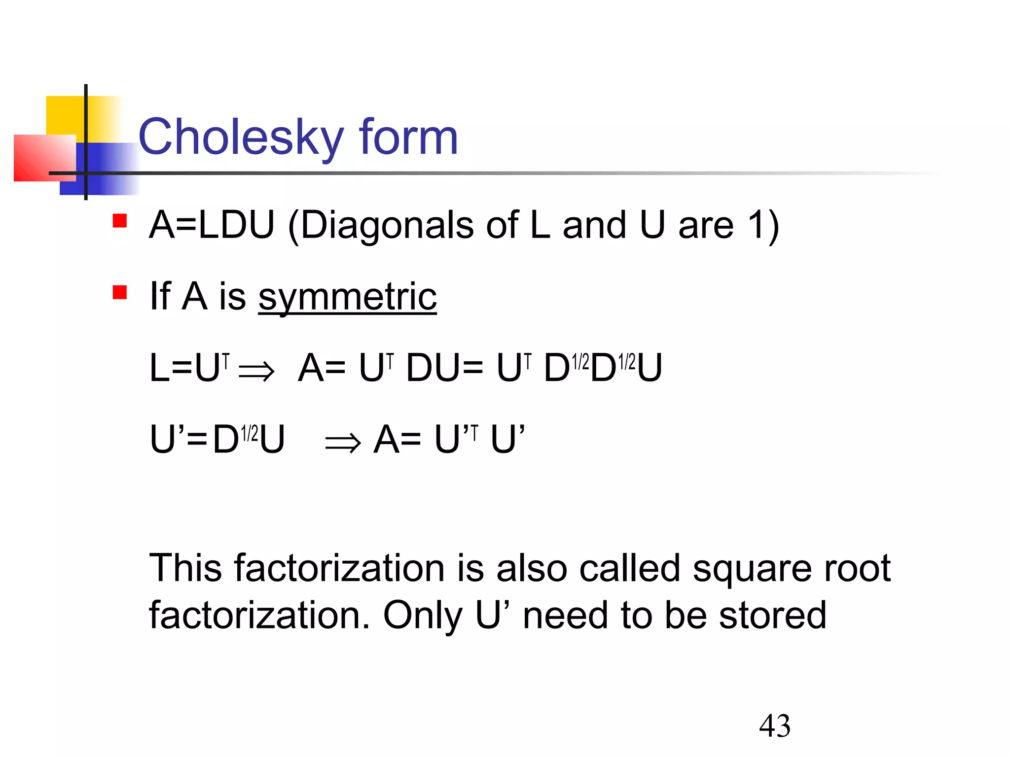
43
Cholesky form
A=LDU(Diagonals of L and U are 1)
If A is symmetric
L=UT
⇒ A= UT
DU= UT
D1/2
D1/2
U
U’=D1/2
U ⇒ A= U’T
U’
This factorization is also called square root
factorization. Only U’ need to be stored
44.
44
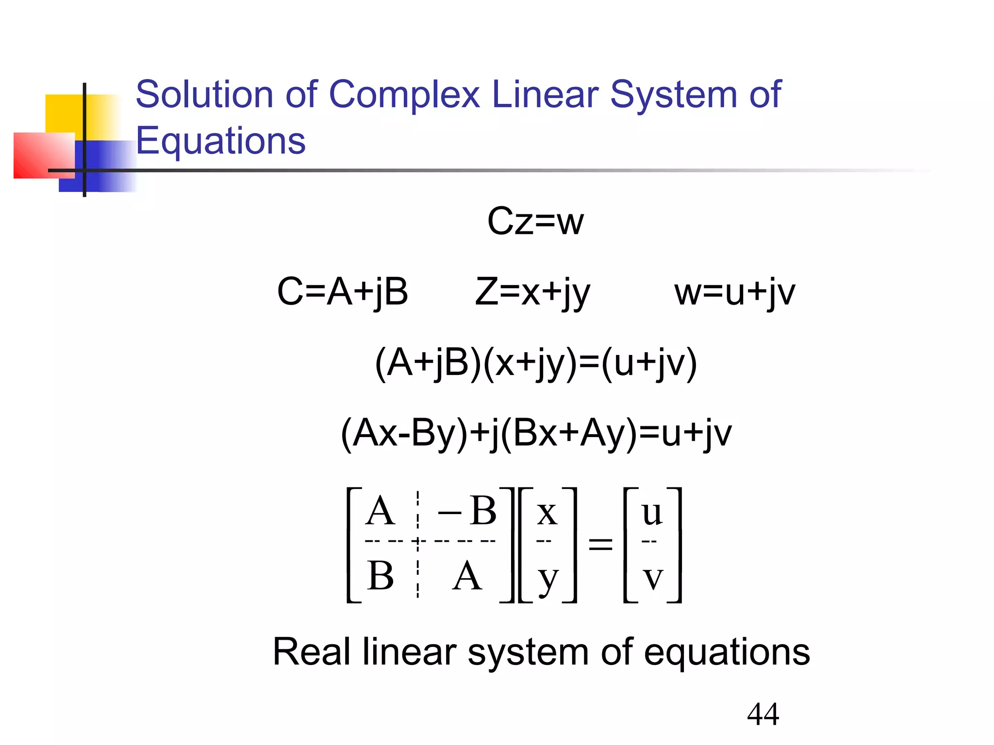
Solution of ComplexLinear System of
Equations
Cz=w
C=A+jB Z=x+jy w=u+jv
(A+jB)(x+jy)=(u+jv)
(Ax-By)+j(Bx+Ay)=u+jv
=
−
v
u
y
x
AB
BA
Real linear system of equations
45.
45
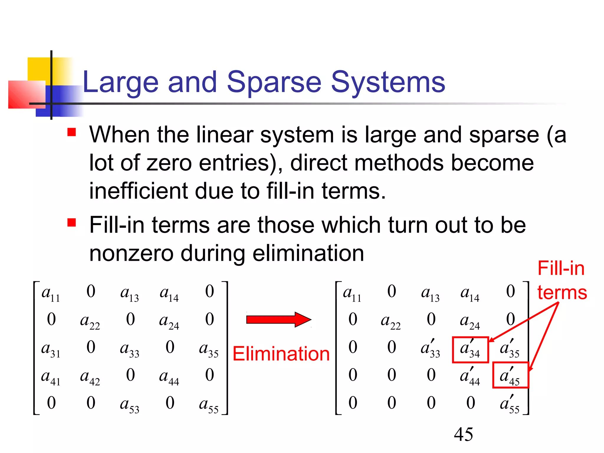
Large and SparseSystems
When the linear system is large and sparse (a
lot of zero entries), direct methods become
inefficient due to fill-in terms.
Fill-in terms are those which turn out to be
nonzero during elimination
5553
444241
353331
2422
141311
000
00
00
000
00
aa
aaa
aaa
aa
aaa
′
′′
′′′
55
4544
353433
2422
141311
0000
000
00
000
00
a
aa
aaa
aa
aaa
Elimination
Fill-in
terms
46.
46
Sparse Matrices
Nodeequation matrix is a sparse matrix.
Sparse matrices are stored very efficiently by
storing only the nonzero entries
When the system is very large (n=10,000) the
fill-in terms considerable increases storage
requirements
In such cases iterative solution methods should
be prefered instead of direct solution methods
![3
Elementary row operations
The following operations applied to the
augmented matrix [A|b], yield an equivalent
linear system
Interchanges: The order of two rows can be
changed
Scaling: Multiplying a row by a nonzero constant
Replacement: The row can be replaced by the sum
of that row and a nonzero multiple of any other row.](https://image.slidesharecdn.com/solutionoflinearsystemofequations-131010034228-phpapp02/75/Solution-of-linear-system-of-equations-3-2048.jpg)
![16
Back substitution algorithm
=
−
−−−−−
)(
)1(
1
)3(
3
)2(
2
)1(
1
1
3
2
1
)(
)(
1
)(
11
)3(
3
)3(
33
)2(
2
)2(
23
)2(
22
)1(
1
)1(
13
)1(
12
)1(
11
0000
000
00
0
n
n
n
n
n
n
n
nn
n
nn
n
nn
n
n
n
b
b
b
b
b
x
x
x
x
x
a
aa
aa
aaa
aaaa
[ ]
1,,2,1
1
1
1
)()(
)(
1
1
)1(
1)1(
11
1)(
)(
−−=
−=
−==
∑+=
−
−
−
−−
−−
−
nnixab
a
x
xab
a
x
a
b
x
n
ik
k
i
ik
i
ii
ii
i
n
n
nn
n
nn
nn
nn
nn
n
n
n](https://image.slidesharecdn.com/solutionoflinearsystemofequations-131010034228-phpapp02/75/Solution-of-linear-system-of-equations-16-2048.jpg)
![39
Gauss-Jordan Elimination
Almost 50% more arithmetic operations than
Gaussian elimination
Gauss-Jordan (GJ) Elimination is prefered
when the inverse of a matrix is required.
Apply GJ elimination to convert A into an
identity matrix.
[ ]IA
[ ]1−
AI](https://image.slidesharecdn.com/solutionoflinearsystemofequations-131010034228-phpapp02/75/Solution-of-linear-system-of-equations-39-2048.jpg)