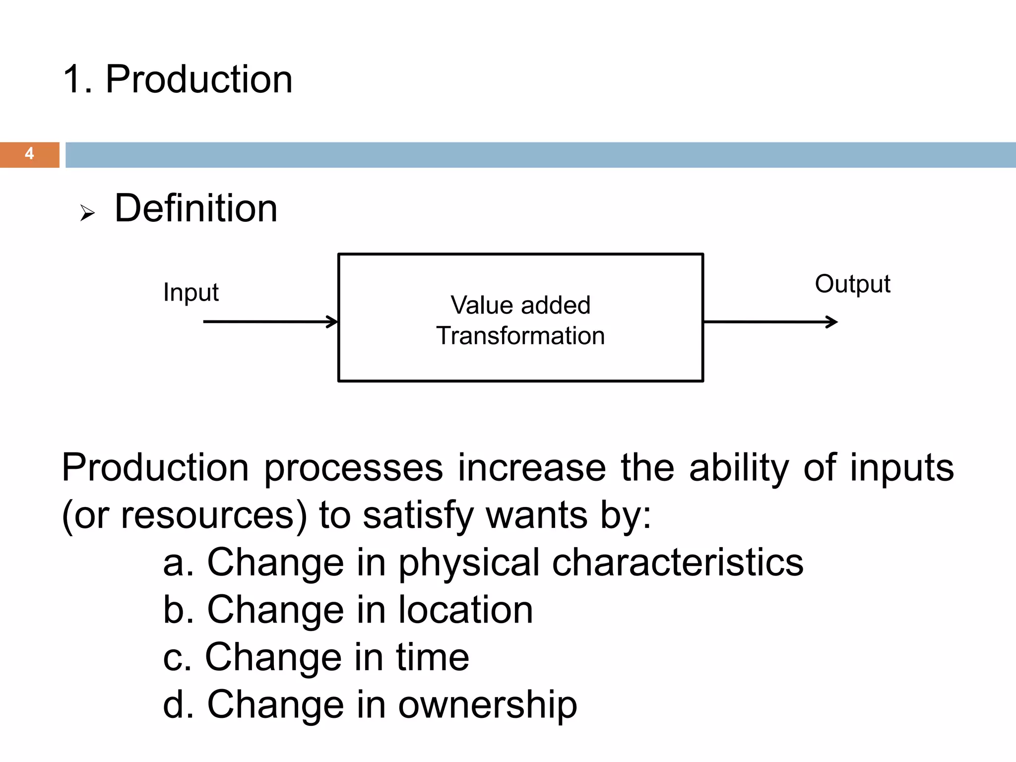
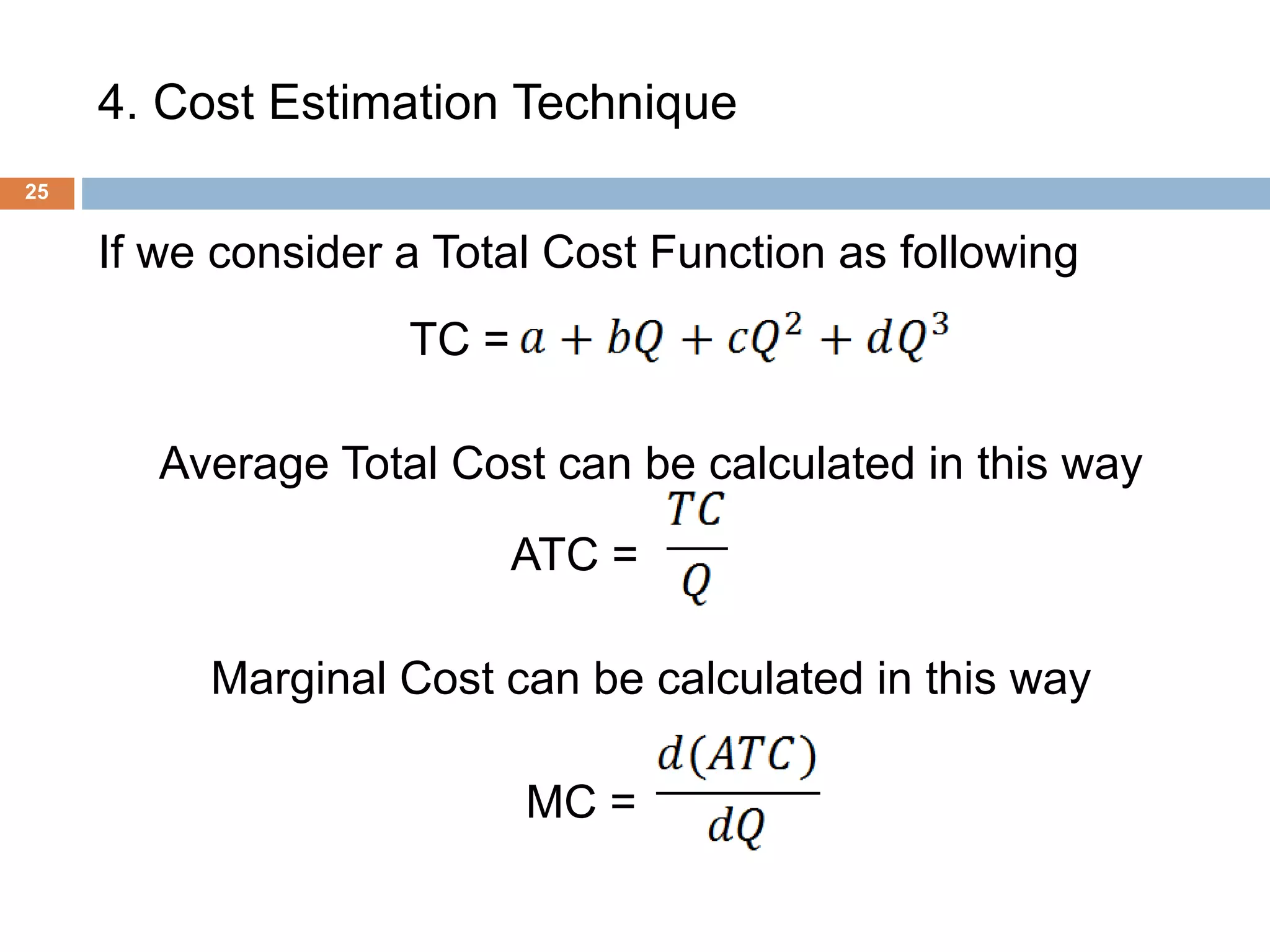
1
Production and Cost Theory
Prepared by
Md. Nasful Huda Prince
Objectives of this presentation
2
 To study about Production theory
 To study about production efficiency
 To study about Cost theory
 To relate the cost with production
 To study to achieve maximum profit for an
organization
 To study to take decision which will result
maximum financial benefit for the organization
Outline of Presentation
3
1. Production
2. Short-run Production and Cost
3. Long-run Production and Cost
4. Cost Estimation Technique
5. Conclusion
1. Production
4
 Definition
Input Output
Value added
Transformation
Production processes increase the ability of inputs
(or resources) to satisfy wants by:
a. Change in physical characteristics
b. Change in location
c. Change in time
d. Change in ownership
1.1. Production
5
 Production Function
Q = f (L,K,Technology,………….)
Cobb-Douglas production function
Q = .
Where, Q represents output,
K represents Capital
and L represents Labor
1.2. Time and Production
6
Generally, four time periods are used in the
analysis of production, they are:
 Market Period
 Short-run
 Long-run
 The very Long-run
Most of the economists consider either Long-run
or short-run.
2. Short-run Production and Cost
2.1. Production in the Short-run
7
Production function can be represented as
Q = f(L,K)
Here, Bar sign upon K indicates that K is fixed.
So the Production function can be represented as
Q = f(L)
2.1. Production in the Short-run
8
Common Terminology:
 Total Product: Sum of total output (Q).
 Average Product: AP = =
 Marginal Product:
MP = =
 Technical Efficiency:
TE =
 Economic Efficiency:
EE=
2.1. Production in the Short-run
9
Fig 1a: Graphical Representation
of Total Product
Fig 1b: Graphical Representation of
Average and Marginal Product
2.2. Sort-run Cost
10
Some common Terms about cost:
 Opportunity Cost
 Implicit and Explicit Cost
 Total Cost (TC)
 Total Fixed Cost (TFC)
 Total Variable Cost (TVC)
 Average Fixed Cost (AFC)
 Average Variable Cost (AVC)
 Marginal Cost (MC)
 Average Total Cost (ATC)
 Total Revenue (TR)
 Marginal Revenue (MR)
2.2. Short-run Cost
11
Fig 2a: Graphical Representation of
Total Cost Curve
Fig 2b: Graphical Representation of AFC,
AVC, AC and MC
2.2. Short-run Cost
12
 Calculation of various cost figure (assuming data)
3. Long-run Production and Cost
13
Long-run Production function can be represented as
Q = f(L,K)
Where, both the inputs are variable but technology is
same.
Cobb-Douglas production function can also be used
to explain this Production Function.
3.1. Isoquant
14
Fig 3: Graphical Representation of Isoquant
The characteristic of Isoquant is that, it is downward sloping.
3.1. Isoquant
15
Fig 4a: Isoquant when inputs
are perfect substitutes
Fig 4b: Isoquant when inputs
are perfect complements
3.2. Marginal Rate of Technical Substitution
(MRTS)
16
MRTS can be defined using following equation
MRTS = - .
It is possible to relate MRTS with Marginal Product
by using following equation
MRTS = - .=
3.3. Isocost Curve
17
Fig 5: Graphical Representation of Isocost
3.3. Isocost Curve
18
Fig 6: Shift of Isocost Curve
3.4. Output Maximization
19
Fig 7: Ouput Maximization for a given level of Cost
3.5. Expansion Path
20
Fig 8: Graphical representation of Expansion Path
3.6. Returns to Scale
21
Consider a production function as following form
Q = f (L,K)
Now if the input will change the variation of out can
be represented as
zQ = f (cL,cK)
Here, c & z are the proportionate change of input
and output
Now, If z>c, Increasing Returns to Scale
If z<c, Decreasing Returns to Scale
If z=c, Constant Returns to Scale
3.7. Economies of Scope (SC)
22
If Joint production cost of two product is C(X,Y) and
C(X) & C(Y) are the individual production cost of
product X & Y the economies of scope will exist if
C(X,Y) < C(X) + C(Y)
The Degree to which SC exist is
SC= .
Diseconomies of scope will exist if
C(X,Y) > C(X) + C(Y)
3.8. Long-run Average and Marginal Cost Curve
23
Fig 9a: Long-run Average and Marginal Cost Curve
3.9. Long-run Average and Marginal Cost Curve
24
Fig 9b: Long-run Average Cost as the Planning Horizon
4. Cost Estimation Technique
25
If we consider a Total Cost Function as following
TC = .
Average Total Cost can be calculated in this way
ATC = .
Marginal Cost can be calculated in this way
MC = .
5. Conclusion
26
 Analysis of production and cost is very important
for an organization.
 A good manager will concentrate on technical
and economic efficiency.
 Study of production and cost will help a
manager to take decision for maximizing
organization profit.
 At last it can be concluded in this way that,
study and improvement of our knowledge about
discussed topics help us to fulfill our
presentation objectives.
27
THANK YOU ALL

Cost theory analysis

  • 1.
    1 Production and CostTheory Prepared by Md. Nasful Huda Prince
  • 2.
    Objectives of thispresentation 2  To study about Production theory  To study about production efficiency  To study about Cost theory  To relate the cost with production  To study to achieve maximum profit for an organization  To study to take decision which will result maximum financial benefit for the organization
  • 3.
    Outline of Presentation 3 1.Production 2. Short-run Production and Cost 3. Long-run Production and Cost 4. Cost Estimation Technique 5. Conclusion
  • 4.
    1. Production 4  Definition InputOutput Value added Transformation Production processes increase the ability of inputs (or resources) to satisfy wants by: a. Change in physical characteristics b. Change in location c. Change in time d. Change in ownership
  • 5.
    1.1. Production 5  ProductionFunction Q = f (L,K,Technology,………….) Cobb-Douglas production function Q = . Where, Q represents output, K represents Capital and L represents Labor
  • 6.
    1.2. Time andProduction 6 Generally, four time periods are used in the analysis of production, they are:  Market Period  Short-run  Long-run  The very Long-run Most of the economists consider either Long-run or short-run.
  • 7.
    2. Short-run Productionand Cost 2.1. Production in the Short-run 7 Production function can be represented as Q = f(L,K) Here, Bar sign upon K indicates that K is fixed. So the Production function can be represented as Q = f(L)
  • 8.
    2.1. Production inthe Short-run 8 Common Terminology:  Total Product: Sum of total output (Q).  Average Product: AP = =  Marginal Product: MP = =  Technical Efficiency: TE =  Economic Efficiency: EE=
  • 9.
    2.1. Production inthe Short-run 9 Fig 1a: Graphical Representation of Total Product Fig 1b: Graphical Representation of Average and Marginal Product
  • 10.
    2.2. Sort-run Cost 10 Somecommon Terms about cost:  Opportunity Cost  Implicit and Explicit Cost  Total Cost (TC)  Total Fixed Cost (TFC)  Total Variable Cost (TVC)  Average Fixed Cost (AFC)  Average Variable Cost (AVC)  Marginal Cost (MC)  Average Total Cost (ATC)  Total Revenue (TR)  Marginal Revenue (MR)
  • 11.
    2.2. Short-run Cost 11 Fig2a: Graphical Representation of Total Cost Curve Fig 2b: Graphical Representation of AFC, AVC, AC and MC
  • 12.
    2.2. Short-run Cost 12 Calculation of various cost figure (assuming data)
  • 13.
    3. Long-run Productionand Cost 13 Long-run Production function can be represented as Q = f(L,K) Where, both the inputs are variable but technology is same. Cobb-Douglas production function can also be used to explain this Production Function.
  • 14.
    3.1. Isoquant 14 Fig 3:Graphical Representation of Isoquant The characteristic of Isoquant is that, it is downward sloping.
  • 15.
    3.1. Isoquant 15 Fig 4a:Isoquant when inputs are perfect substitutes Fig 4b: Isoquant when inputs are perfect complements
  • 16.
    3.2. Marginal Rateof Technical Substitution (MRTS) 16 MRTS can be defined using following equation MRTS = - . It is possible to relate MRTS with Marginal Product by using following equation MRTS = - .=
  • 17.
    3.3. Isocost Curve 17 Fig5: Graphical Representation of Isocost
  • 18.
    3.3. Isocost Curve 18 Fig6: Shift of Isocost Curve
  • 19.
    3.4. Output Maximization 19 Fig7: Ouput Maximization for a given level of Cost
  • 20.
    3.5. Expansion Path 20 Fig8: Graphical representation of Expansion Path
  • 21.
    3.6. Returns toScale 21 Consider a production function as following form Q = f (L,K) Now if the input will change the variation of out can be represented as zQ = f (cL,cK) Here, c & z are the proportionate change of input and output Now, If z>c, Increasing Returns to Scale If z<c, Decreasing Returns to Scale If z=c, Constant Returns to Scale
  • 22.
    3.7. Economies ofScope (SC) 22 If Joint production cost of two product is C(X,Y) and C(X) & C(Y) are the individual production cost of product X & Y the economies of scope will exist if C(X,Y) < C(X) + C(Y) The Degree to which SC exist is SC= . Diseconomies of scope will exist if C(X,Y) > C(X) + C(Y)
  • 23.
    3.8. Long-run Averageand Marginal Cost Curve 23 Fig 9a: Long-run Average and Marginal Cost Curve
  • 24.
    3.9. Long-run Averageand Marginal Cost Curve 24 Fig 9b: Long-run Average Cost as the Planning Horizon
  • 25.
    4. Cost EstimationTechnique 25 If we consider a Total Cost Function as following TC = . Average Total Cost can be calculated in this way ATC = . Marginal Cost can be calculated in this way MC = .
  • 26.
    5. Conclusion 26  Analysisof production and cost is very important for an organization.  A good manager will concentrate on technical and economic efficiency.  Study of production and cost will help a manager to take decision for maximizing organization profit.  At last it can be concluded in this way that, study and improvement of our knowledge about discussed topics help us to fulfill our presentation objectives.
  • 27.