Thesis Report.pdf

TRIBHUVAN UNIVERSITY
INSTITUTE OF ENGINEERING
PULCHOWK CAMPUS
DEPARTMENT OF ELECTRICAL ENGINEERING
MASTER OF SCIENCE IN POWER SYSTEM ENGINEERING
ROLL NO.: 074MSPSE017
SMART RECONFIGURATION OF DISTRIBUTION NETWORKS HANDLING DG
PENETRATION FOR POWER LOSS MINIMIZATION AND VOLTAGE PROFILE
IMPROVEMENT
THESIS REPORT
BY
SURAJ KUMAR DHUNGEL
Thesis Supervisor
Prof. Dr. Nava Raj Karki
February, 2021

ii | P a g e
ABSTRACT
Power loss minimization and voltage stability improvement are important areas of power systems
due to existing transmission line contingency, financial loss of utility and power system blackouts.
Distribution network reconfiguration (DNR) can significantly reduce power losses, improve the
voltage profile, and increase the power quality. DNR studies require implementation of the power
flow analysis and complex optimization procedures capable of handling large combinatorial
problems. In addition, optimal allocation (i.e. siting, sizing, and operating power factor) of
Distributed Generation (DG) is one of the best ways to strengthen the efficiency of power system
along with network reconfiguration. Power system operators and researchers put forward their
efforts to solve the distribution system problem related to power loss, energy loss, voltage profile,
and voltage stability based on optimal DG allocation. Furthermore, optimal DG allocation secures
distribution system from unwanted events and allows the operator to run the system in islanding
mode.
The size of the distribution network influences the type of the optimization method to be applied.
In particular, straight forward approaches can be computationally expensive or even prohibitive
whereas heuristic or metaheuristic approaches can yield acceptable results with less computation
cost. In the problems like DNR, there is extensive search procedure involved in finding the optimum
solution. In addition, the solution improves in various stages of search procedure and in each
iteration. In the optimization problems like the one in this thesis work, large number of variables
have to be optimized. Distribution network reconfiguration and placement of DGs involves fourteen
variables when five disconnecting switches and three DGs are considered – five for the
disconnecting switches, three variables for the placement of DGs, three variables for the sizing of
DGs, and three variables for the optimum power factor of DGs. Only the most efficient algorithms
are able to find the optimum solution in minimum iteration and minimum time. Artificial Bee
Colony (ABC) algorithm has been used in this thesis work as it is very easy to implement and
efficient in finding optimum solution when compared to other popular metaheuristic algorithms like
Genetic Algorithm, and Particle Swarm Optimization Algorithm.

iii | P a g e
Firstly, the bus voltage profile, and power loss was determined for the system taken into
consideration (Base Case). Then, distribution network reconfiguration was implemented in standard
IEEE buses (Case I). In the next step, DGs were incorporated in the standard IEEE buses and
reconfiguration was designed. In that analysis, initially only the case of DG installation was
analyzed (Case II). Afterwards, the case of DG installation after reconfiguration was taken (Case
III). Then, the case of reconfiguration after DG installation was studied (Case IV). Finally, the case
of simultaneous reconfiguration after DG installation was analyzed (Case V).
First, IEEE 33 Bus System was considered and the base case power loss for the system was 202.67
kW. For the Case I, the power loss reduced by 30.93%. When considering DGs capable of injecting
active power only, the power loss was reduced by 59.16%, 71.24%, 68.81%, and 71.49%
respectively for Case II, Case III, Case IV, and Case V respectively. The minimum bus voltage
improved significantly and was at least 0.951 pu for Case II, Case III, Case IV, and Case V. When
considering DGs capable of injecting both active power and reactive power, the power loss was
reduced by 86.86%, 89.29%, 91.60%, and 92.93% for Case II, Case III, Case IV, and Case V
respectively. The minimum bus voltage also improved significantly and was at least 0.966 pu for
Case II, Case III, Case IV, and Case V.
In the next step, IEEE 69 Bus System was considered and the base case power loss for the system
was 225 kW. For the Case I, the power loss reduced by 56.17%. When considering DGs capable of
injecting active power only, the power loss was reduced by 66.93%, 83.21%, 80.92%, and 83.52%
respectively for Case II, Case III, Case IV, and Case V respectively. The minimum bus voltage
improved significantly and was at least 0.978 pu for Case II, Case III, Case IV, and Case V. When
considering DGs capable of injecting both active power and reactive power, the power loss was
reduced by 95.16%, 95.96%, 96.56%, and 97.45% for Case II, Case III, Case IV, and Case V
respectively. The minimum bus voltage also improved significantly and was at least 0.987 pu for
Case II, Case III, Case IV, and Case V.
Finally, Daachhi feeder of Kathmandu valley was taken as a subject to apply the theoretically
proven technique of reconfiguration and DG incorporation to optimize voltage profile and power
loss. The base case power loss for the system was 197.026 kW. For the Case I, the power loss
reduced by 5.30%. When considering DGs capable of injecting active power only, the power loss

iv | P a g e
was reduced by 40.17%, 51.18%, 41.94%, and 51.43% respectively for Case II, Case III, Case IV,
and Case V respectively. The minimum bus voltage improved significantly and was at least 0.968
pu for Case II, Case III, Case IV, and Case V. When considering DGs capable of injecting both
active power and reactive power, the power loss was reduced by 76.30%, 91.89%, 76.57%, and
92.71% for Case II, Case III, Case IV, and Case V respectively. The minimum bus voltage also
improved significantly and was at least 0.973 pu for Case II, Case III, Case IV, and Case V. Overall
findings showed that performing simultaneous distribution network reconfiguration and allocation
of DGs yielded best results in reducing system loss and improving bus voltage profile, which is in-
line with objectives of this thesis work.

v | P a g e
ACKNOWLEDGEMENTS
The successful completion of this thesis work would not have been possible without the guidance and
support of many people and I am extremely grateful to have got this all along the way of my thesis
work. I would like to offer my thankfulness to my thesis supervisor Prof. Dr. Nava Raj Karki for his
invaluable guidance, support, and encouragement throughout this thesis work and research process. I
am grateful for his mentorship and friendly guidance not only during this thesis, but also throughout
the master’s program.
I would like to express my sincere appreciation to all teachers and staff of Department of Electrical
Engineering, Pulchowk Campus. In addition, I would like to express my gratitude to Engineer Saru
Bastola of Baneshwor Distribution Centre, Nepal Electricity Authority for her support during field
visits and data collection of Daachhi feeder.
Last but not the least, I would like to acknowledge my family and friends who have made a
contribution directly or indirectly to complete this thesis work.

vi | P a g e
Table of Contents
ABSTRACT ____________________________________________________________________ ii
ACKNOWLEDGEMENTS ________________________________________________________ v
List of Tables__________________________________________________________________viii
List of Figures __________________________________________________________________ix
CHAPTER I: INTRODUCTION __________________________________________________ 1
1.1 Introduction ___________________________________________________________ 1
1.2 Problem Statement ______________________________________________________ 3
1.3 Objectives of the Project__________________________________________________ 4
1.4 Scope ________________________________________________________________ 4
1.5 Outline of the Report ____________________________________________________ 4
CHAPTER II: REVIEW OF LITERATURE ________________________________________ 6
2.1 Introduction ___________________________________________________________ 6
2.2 The Distribution Power System ____________________________________________ 9
2.3 Distribution Network Reconfiguration and Optimal Distributed Generation Allocation 10
2.4 Voltage Stability Index of Radial Distribution Networks _______________________ 12
2.5 Artificial Bee Colony Algorithm __________________________________________ 15
2.5.1 Producing initial food source sites _________________________________________ 16
2.5.3 Calculating probability values involved in probabilistic selection_________________ 17
2.5.4 Food source site selection by onlookers based on the information provided by employed
bees 18
2.5.5 Abandonment criteria: Limit and scout production ____________________________ 18
CHAPTER III: METHODOLOGY _______________________________________________ 20
3.1 Power Distribution System Modeling ______________________________________ 20
3.2 Short-listing of the candidate buses for installation of DGs______________________ 21
3.3 Cases of Analysis ______________________________________________________ 21
3.4 Problem Formulation ___________________________________________________ 23

vii | P a g e
3.5 Solution Variables supplied to ABC algorithm _______________________________ 23
3.6 Steps in ABC algorithm _________________________________________________ 25
3.7 Checking Radial Topology_______________________________________________ 26
CHAPTER IV: SYSTEM UNDER CONSIDERATION, SOFTWARE AND TOOLS______ 34
4.1 Systems under consideration _____________________________________________ 34
4.2 Software and Tools Used ________________________________________________ 45
CHAPTER V: RESULTS AND DISCUSSIONS_____________________________________ 46
5.1 For IEEE 33 Bus System ________________________________________________ 46
5.2 For IEEE 69 Bus System ________________________________________________ 49
5.3 For Daachhi Feeder of Kathmandu ________________________________________ 52
CHAPTER VI: CONCLUSION __________________________________________________ 54
REFERENCES ________________________________________________________________ 56
Appendix-1: Results for IEEE 33 Bus System _______________________________________ 59
Appendix-2: Results for IEEE 69 Bus System _______________________________________ 71
Appendix-3: Results for Daachhi Feeder ___________________________________________ 83

viii | P a g e
List of Tables
Table 1: System data for 33-bus radial distribution network (‘*’ denotes a tie-line)____________________________ 36
Table 2: System data for 69-bus radial distribution network (‘*’ denotes a tie-line)____________________________ 37
Table 3: System data for distribution network of Daachhi feeder of Kathmandu valley (‘*’ denotes a tie-line) _______ 43
Table 4: Results comparison for IEEE 33 Bus System ___________________________________________________ 48
Table 5: Results comparison for IEEE 69 Bus System ___________________________________________________ 50
Table 6: Results comparison for Daachhi feeder of Kathmandu when considering three different types of DGs ______ 52

ix | P a g e
List of Figures
Figure 1: Flowchart of ABC algorithm ............................................................................................................................. 19
Figure 2: Flowchart for checking radial topology............................................................................................................ 28
Figure 3: Choices for type of analysis............................................................................................................................... 29
Figure 4: Options to choose data set................................................................................................................................. 29
Figure 5: Windows for user inputs .................................................................................................................................... 30
Figure 6: Result format ..................................................................................................................................................... 31
Figure 7: Branch Current format...................................................................................................................................... 32
Figure 8: Voltage Profile (numbers) format...................................................................................................................... 32
Figure 9: Voltage Profile Comparison (Before and After) format .................................................................................... 33
Figure 10: IEEE 33 Bus Test System................................................................................................................................. 34
Figure 11: IEEE 69 Bus Test System................................................................................................................................. 35
Figure 12: GIS Plot of Daachhi Feeder ............................................................................................................................ 41
Figure 13: SLD of Daachhi feeder .................................................................................................................................... 42
Figure 14: Result window for N/W Reconfiguration only for IEEE 33 Bus System when considering all DGs inject active
power only ......................................................................................................................................................................... 59
Figure 15: Bus Voltage Profile for N/W Reconfiguration only for IEEE 33 Bus System when considering all DGs inject
active power only............................................................................................................................................................... 60
Figure 16: Result window for DG Placement only for IEEE 33 Bus System when considering all DGs inject active power
only.................................................................................................................................................................................... 61
Figure 17: Bus Voltage Profile for DG Placement only for IEEE 33 Bus System when considering all DGs inject active
power only ......................................................................................................................................................................... 62
Figure 18: Result window for First N/W Reconfiguration and then DG Placement for IEEE 33 Bus System when
considering all DGs inject active power only.................................................................................................................... 63
Figure 19: Bus Voltage Profile Result for First N/W Reconfiguration and then DG Placement for IEEE 33 Bus System
when considering all DGs inject active power only .......................................................................................................... 64
Figure 20: Result window for First DG Placement and then N/W Reconfiguration for IEEE 33 Bus System when
Figure 21: Bus Voltage Profile for First DG Placement and then N/W Reconfiguration for IEEE 33 Bus System when
Figure 22: Result window for Simultaneous N/W Reconfiguration and DG Placement for IEEE 33 Bus System when
Figure 23: Bus Voltage Profile for Simultaneous N/W Reconfiguration and DG Placement for IEEE 33 Bus System when
considering all DGs inject both active and reactive power............................................................................................... 69

x | P a g e
Figure 25: Voltage Profile for Simultaneous N/W Reconfiguration and DG Placement for IEEE 33 Bus System when
Figure 26: Result window for N/W Reconfiguration only for IEEE 69 Bus System when considering all DGs inject active
power only ......................................................................................................................................................................... 71
Figure 27: Bus Voltage Profile for N/W Reconfiguration only for IEEE 69 Bus System when considering all DGs inject
Figure 28: Result window for DG Placement only for IEEE 69 Bus System when considering all DGs inject active power
only.................................................................................................................................................................................... 73
Figure 29: Bus Voltage Profile for DG Placement only for IEEE 69 Bus System when considering all DGs inject active
power only ......................................................................................................................................................................... 74
Figure 30: Result window for First N/W Reconfiguration and DG Placement for IEEE 69 Bus System when considering
all DGs inject active power only ....................................................................................................................................... 75
Figure 31: Bus Voltage Profile for First N/W Reconfiguration and DG Placement for IEEE 69 Bus System when
Figure 32: Result window for First DG Placement and then N/W Reconfiguration for IEEE 69 Bus System when
Figure 33: Bus Voltage Profile for First DG Placement and then N/W Reconfiguration for IEEE 69 Bus System when
Figure 35: Bus Voltage Profile for Simultaneous N/W Reconfiguration and DG Placement for IEEE 69 Bus System when
Figure 37: Voltage Profile for Simultaneous N/W Reconfiguration and DG Placement for IEEE 69 Bus System when
Figure 38: Result window for N/W Reconfiguration only for Daachhi feeder .................................................................. 83
Figure 39: Bus Voltage Profile for N/W Reconfiguration only for Daachhi feeder .......................................................... 84
Figure 40: Result window for DG placement only for Daachhi feeder when DGs inject active power only .................... 85
Figure 41: Bus Voltage Profile for DG placement only for Daachhi feeder when DGs inject active power only ............ 86
Figure 42: Result window for First N/W Reconfiguration and then DG Placement for Daachhi feeder when DGs inject
Figure 43: Bus Voltage Profile for First N/W Reconfiguration and then DG Placement for Daachhi feeder when DGs
inject active power only..................................................................................................................................................... 88
Figure 44: Result window for First DG Placement and then N/W Reconfiguration for Daachhi feeder when DGs inject

xi | P a g e
Figure 45: Bus Voltage Profile for First DG Placement and then N/W Reconfiguration for Daachhi feeder when DGs
Figure 46: Result window for Simultaneous N/W Reconfiguration and DG placement for Daachhi feeder when DGs
Figure 47: Bus Voltage Profile for Simultaneous N/W Reconfiguration and DG placement for Daachhi feeder when DGs
Figure 48: Result window for Simultaneous N/W Reconfiguration and DG placement for Daachhi feeder when DGs
inject both active power and reactive power ..................................................................................................................... 93
Figure 49: Bus Voltage Profile for Simultaneous N/W Reconfiguration and DG placement for Daachhi feeder when DGs
inject both active power and reactive power ..................................................................................................................... 94

1 | P a g e
CHAPTER I: INTRODUCTION
1.1 Introduction
Utilities in the developing and under-developed countries face capital shortage for generation and
transmission system amid disproportionate load growth. Efficiency of the power system depends on
the performance of the transmission and distribution network. Higher the power losses of the
transmission and distribution systems, lower is the efficiency of the power system. Power losses
account for financial loss of the utilities - lower the losses, higher the revenue. For utilities facing lack
of capital, effective and smart utilization of existing infrastructure with minimal improvements brings
two important benefits – first, it delays the capital requirement to reinforce the existing system; second,
it generates additional revenue which can serve as a part of capital requirement to reinforce the existing
system. Meanwhile, after deregulation and privatization of the power system, another common
problem observed in distribution systems is the lack of reactive power sources in the system [1].
Barring installation of reactive power sources exclusively to cater reactive power load, reactive power
generated by distributed generators can reduce the reactive power supplied from the grid.
Network reconfiguration is the process of changing the topology by altering the open/closed status of
switches, so as to find a radial operating structure that minimizes the losses and improves the
voltage stability while satisfying the operating constraints. Distribution network reconfiguration
(DNR) is the best methodology that can reduce power loss and improve power quality for the efficient
operation of power distribution systems using existing resources. Radial distribution networks often
feature sectionalizing switches and tie switches mainly used for fault isolation, power supply recovery,
and system reconfiguration. These switches allow for reconfiguring the topology of the network, with
the objectives being reduction of power losses, load balancing, and voltage profile improvement and
increasing reliability of the system [2]. A network reconfiguration is a complex non-linear
combinatorial problem as the solution is a large combination search space of open switches. The
complexity increases with increase in network size. It is why, artificial intelligence and meta-heuristic
optimization techniques are efficient to solve such problems as compared to analytical methods.
On the other hand, introduction of the smart grid, and the liberalization of energy markets has allowed
interconnection Distributed Generations at distribution end. The DGs are mainly of renewable energy

2 | P a g e
type, dominated by solar and wind power plants. Distribution companies try to minimize real losses
in order to obtain profit rather than paying a penalty. Therefore, a host of research publications has
proposed numerous methods for active power loss minimization of distribution systems. To maintain
voltage profile of the system within a given minimum level, sufficient reactive power support is
needed, which in turn also raises the stability and reliability of the system. In such a situation, it is
imperative to introduce a variety of innovative technologies for optimal utilization of existing
resources and resolution of reported issues to meet the target of load demand with power quality and
in a cost-effective way [1]. One of the latest ways to handle these issues in economical and reasonable
time is the optimal allocation of distributed generation in power systems. In a power system composed
of distributed energy resources, much smaller amounts of energy are produced by numerous small,
modular energy conversion units, which are often located close to the point of end use. Both demand
and distribution generation are directly connected to the distribution network. Besides, DG units, local
responsive demands, and storage systems can be operated stand alone or integrated into the electricity
grid [3]. Combination of multiple methodologies such as distribution reconfiguration and optimal
allocation of DGs have been proposed to increase the benefits; however, the practical complexity of
implementing such combination of methodologies increases significantly.

3 | P a g e
1.2 Problem Statement
The performance of distribution system becomes inefficient due to the reduction in voltage magnitude
and increase in distribution losses. Since the distribution power system is the final stage of the
distribution process from the source to the individual customer, it has seemed to contribute the greatest
amount of power loss which finally results into the instability of the system. Many researchers have
been focusing on power loss minimization in the distribution system by using various methods.
In the context of Nepal, it is not a necessity but a compulsion to integrate DGs if they are willing to
integrate in the existing network. Nepal Electricity Authority (NEA) has released its guidelines in
April, 2016 for interconnection of photovoltaic to distribution network. In February 2018, Ministry of
Energy released standard procedure for connection of alternative energy to the existing grid.
According to the guideline, energy producers willing to sell energy for solar capacity above 500 watts
may apply to NEA for interconnection through net metering. Following these: CIAA- Tangal (514
kW), ICIMOD- Khumaltar (92 kW) are already installed and ready for integration in the distribution
network while NMB Bank- Babarmahal (50kW) is due for PPA with NEA. NEA has already
integrated 600 kW solar plant installed at Dhobighat under Kathmandu Upatyaka Khanepani Limited
(KUKL), 100 kW solar plant installed at NEA Training Center, and 60 kW solar installed at Bir
Hospital in the distribution network.
Among the various methods of loss minimization, the recent method used is reconfiguration
Distribution Network Reconfiguration capable of handling Distributed Generation penetration has
been proposed in this thesis work. Distribution Network Reconfiguration alters the present connection
of branches between the buses and proposes a new configuration of connection which gives the
shortest path between the source and the load, resulting minimum power loss. And, proper allocation
of Distributed Generations facilitates as on-site supplier of active power and reactive power to the
loads. That way, all the demand power doesn’t have to travel from the grid to the load, resulting
minimum power loss. This thesis work shall give optimum reconfiguration of the distribution network
along with proper siting, sizing, and operating power factor of DGs if there are new ones to come.
Even if there are existing DGs, the outcome of this thesis will propose optimum reconfiguration of
the network to minimize power loss and improve voltage profile.

4 | P a g e
1.3 Objectives of the Project
The objective of this thesis is to study simultaneous network reconfiguration, and optimum allocation
(placement, sizing & operating power factor) of distributed generations so as to minimize power loss
and optimize voltage profile using Artificial Bee Colony (ABC) algorithm-based computer program.
1.4 Scope
At the end of this work, a software/program is developed that can take the inputs of any number of
buses of a practical distribution system. That way, smaller to larger, both sorts of systems can be
reconfigured using the outputs given at the end of this work.
In addition, the effect of incorporation of distribution generations can be seen along with distribution
network reconfiguration. Also, whether the distribution generation should be introduced or not for the
purpose of reducing power loss and voltage drop can be analyzed. Or, whether the network
reconfiguration is needed or not can be analyzed when distributed generations are added.
1.5 Outline of the Report
This thesis report is organized in six chapters. Chapter I deals with the basic concept of need for
distribution network reconfiguration, and distributed generations. It emphasizes on the optimum use
of existing infrastructures to reduce power loss and optimize voltage profile.
Chapter II reviews the past works conducted in similar subjects that of this thesis work by various
authors in the past. It highlights how and when the reconfiguration problem was considered to solve
power loss and voltage drop issues, and how incorporation of DGs assisted the same.
In Chapter III, overall methodology followed to fulfil the objective of this thesis work is explained. It
explains the algorithm adopted in this thesis work and the cases considered. It also explains how the
search space for optimization was increased using shortlisting criteria of candidate buses for DG
installation.

5 | P a g e
In Chapter IV, systems under consideration, and software and tools used are explained. It shows the
single line diagram and the bus/branch data of the systems considered. It also explains about the
software and tools used for this thesis work.
Chapter V presents results and discussion of results for various scenarios considered in this thesis
work. First, it compares the results obtained in this thesis work against the results in the reference
papers. Later, it demonstrates the method used in this thesis work to improve the power loss and
voltage profile of a practical distribution system of Kathmandu, Nepal.
Finally, Chapter VI concludes the study conducted for various systems under consideration under
various scenarios. It shows that the objectives of this thesis work are fulfilled.

6 | P a g e
CHAPTER II: REVIEW OF LITERATURE
2.1 Introduction
The distribution network transfers the electrical energy directly from the intermediate transformer
substations to consumers. Electric distribution systems are becoming large and complex leading to
higher system losses and poor voltage regulation. In general, almost 10–13% of the total power
generated is lost as I2
R losses at the distribution level, which in turn, causes increase in the cost of
energy and poor voltage profile along the distribution feeder. Therefore, it becomes important to
improve the reliability of the power transmission in distribution networks. While the transmission
networks are often operated with loops or radial structures, the distribution networks are always
operated radially. By operating in radial configuration, short-circuit current is reduced significantly.
The restoration of the network from faults is implemented through the closing/cutting manipulations
of electrical switch pairs located on the loops, consequently. Therefore, there are many switches on
the distribution network.
Distribution network reconfiguration (DNR) is the process of varying the topological arrangement of
distribution feeders by changing the open/closed status of sectionalizing and tie switches while
respecting system constraints upon satisfying the operator’s objectives. DG units are small generating
plants connected directly to the distribution network or on the customer site of the meter. The
number of DG units installed in the distribution system has been increasing significantly, and their
technical, economical, and environmental impacts on power system are being analyzed. The most
critical factors that influence the technical and economic impacts are type, size, and location of DG
units in power system.
The most common methods used for voltage stability enhancement and power loss reduction in power
distribution systems are network reconfiguration and DG placement. The configuration of the
network, placement and size of DG units should be optimal to maximize the benefits and reduce their
impact on the power system. Thus, the optimal integration between these two problems becomes a
significant and complex problem. The results in [4] proves that the simultaneous reconfiguration with
DG allocation give better results out of all other combinations with or without DGs.

7 | P a g e
Many researchers solved the network reconfiguration problems using different methods for the last
two decades [1]. Authors in [5] proposed a pioneering solution to solve the network reconfiguration
problem for loss minimization using a branch and bound-type optimization technique. Later on,
several optimization algorithms have been developed for loss minimization and/or voltage profile
improvement. Authors in [6] used a discrete artificial bee colony algorithm to find the maximum
loadable point by optimizing the distribution network, and also used continuation power flow along
with graph theory to compute power flow. In [7], authors solved the reconfiguration problem assuming
a series fault at a bus using Bacterial Foraging Optimization Algorithm (BFOA). Authors in [8]
proposed modified honey bee mating optimization algorithm to investigate the network
reconfiguration problem with the consideration effect of the renewable energy sources. In the very
latest researches, a new non-revisiting genetic algorithm had been proposed for solving the
reconfiguration problem [9].
DG units are small generating plants connected directly to the distribution network or on the customer
site of the meter. DGs has many advantages over centralized power generation including reduction in
power losses, improved voltage profile, system stability improvement, pollutant emission reduction
and relieving transmission and distribution system congestion. After deregulation of power system,
many power companies are investing in small-scale renewable energy resources such as wind, photo-
voltaic cells, micro turbines, small hydro turbines, etc. to meet the active power demand (MW) as well
as to earn a profit [1].
In distribution systems, DG can provide benefits for the consumers as well as for the utilities,
especially in sites where the central generation is impracticable or where there are deficiencies in the
transmission system. In this context, the utility obligation of providing access to distribution network
for independent producers to install DG units confronts with the need of controlling the network and
guaranteeing appropriate security and reliability levels. The expected benefits of distributed energy
sources are:
• Increased penetration of RES and other DG will help security of supply by reducing energy
imports and building a diverse energy portfolio.

8 | P a g e
• Wide-scale use of RES will reduce fossil fuel consumption and greenhouse gas emissions as
well as noxious emissions such as oxides of Sulphur and nitrogen (SOx/NOx), thereby
benefiting the environment in a power system dominated by the thermal power generation.
• DG helps bypass ‘‘congestion’’ in existing transmission grids. DG could serve as a substitute
for investments in transmission and distribution capacity. DG can postpone the need for
new infrastructure. Because of opportunities for integration in buildings, PV development
often occurs in the same location as demand. In such cases, if production output is concurrent
with demand—such as demand for air-conditioning in hot regions—network reinforcement
may be unnecessary while generation remains in the same order of magnitude as
demand. Moreover, normal development of the grid in response to growing demand may also
be postponed or even avoided as DG has the net effect of decreasing demand in that
area.
• On-site production reduces the amount of power that must be transmitted from centralized
plant, and avoids resulting transmission losses and distribution losses as well as the
transmission and distribution costs.
• DG can provide network support or ancillary services. The connection of distributed
generators to networks generally leads to a rise in voltage in the network. In areas where
voltage support is difficult, installation of a distributed generator may improve quality of
supply [3].
The number of DG units installed in the distribution system has been increasing significantly, and
their technical, economical, and environmental impacts on power system are being analyzed. The most
critical factors that influence the technical and economic impacts are type, size, and location of DG
units in power system. Authors in [10] and [11] presented an analytical and improved analytical
expression for finding the optimal location and size of DG units for reducing power loss along with
methodologies for identifying the optimal location. Authors in [12] proposed Particle Swarm
Optimization (PSO) based technique to solve the optimal placement of different types of DGs for
power loss minimization. In [13], the authors used Fireworks Algorithm (FWA) to solve the network
reconfiguration problem combined with placement and sizing of DGs.

9 | P a g e
All the above researches focused only on the optimization of either distribution network or the DG
placement. However, the objective was to minimize the power loss and/or to improve the voltage
stability, network reconfiguration usually did not take the DG units into consideration and vice versa.
To benefit the whole distribution network effectively, it is necessary to integrate both the network
reconfiguration and DG placement problems. The novelty of this thesis is that it uses recently
developed Artificial Bee Colony (ABC) algorithm for solving the distribution system network
reconfiguration together with DG placement for the problem of power loss minimization and voltage
stability enhancement.
2.2 The Distribution Power System
Power flow calculation is an essential numerical (often nonlinear) analysis needed when making
power systems studies. The practical application of proposed methods on the improvement of the
power distribution network (e.g. power loss reduction, increase in reliability levels, voltage profile
improvement) typically require many power flow analysis algorithms runs. The power flow
methodologies applied to distribution systems will have to adapt to the nature of the distribution
network, in strict terms, they will be demanded to include single phase and three phase unbalanced
system analysis, as well as the influence of distributed generation interconnection. In Distribution
system reconfiguration, the objectives are to minimize power losses and enhance voltage profile,
consequently, power flow analysis becomes an essential procedure to be performed in order to obtain
steady state electrical characteristics of the distribution system as consequence of reconfiguration.
Often, power flow analysis methodology applied to transmission systems is mainly comprised by the
Gauss-Seidel, Newton-Raphson (NR) and its decoupled version. These power flow methods are
typically used assuming a balanced system, consequently using a single-phase representation of a
three-phase system. Due to the particular characteristics of distribution systems (i.e. unbalanced loads,
radial topology, often un-transposed lines, distributed generation, etc.) the assumptions made in the
analysis of transmission systems fail to be extrapolated to the distribution system. Thereupon, a power
flow method considering three phase unbalanced networks must be considered for its application in
distribution systems. The forward/backward methods (a popular power flow method applied to
distribution systems) are capable of performing power flow analysis assuming unbalanced phase
systems, however, it is limited to radial networks and does not have the ability to consider the influence

10 | P a g e
of distributed generation, given in both, phase frame and sequence frame references. On the other
hand, Newton based methods typically can deal with any topology type (i.e. radial, weakly meshed
and meshed) and can consider the influence of distributed generation, in both, phase frame and
sequence frame references. The main attribution to the success of the modified Newton method in
distribution systems is the representation of the Jacobian matrix which is created based on the nature
of the network topology. MATPOWER toolbox was used in this thesis work to compute power flows
for various configuration of open/closed switches. The injection of various DGs of various capacities
at various locations can easily be incorporated in power flow studies in MATPOWER. Distribution
reconfiguration for power loss reduction is implemented based on a radial network.
2.3 Distribution Network Reconfiguration and Optimal Distributed
Generation Allocation
The electric power distribution network is an elemental component of the power distribution system.
It deserves particular attention for the most significant challenges, both design- and operational-wise,
emerge at this level. One particular area of interest for power engineers working on distribution
systems is finding feasible solutions for power loss reduction; power losses in distribution systems
can account for up to 70 percent of the total power losses, consequently increasing the operational
costs of the system. Introduction of the smart grid (SG) concept that aims at supporting the transition
into a safe, efficient and sustainable power system, requires the use of computational intelligence
methods to meet the aforementioned objectives. Distribution network reconfiguration (DNR) has been
shown to be a feasible approach, often involving computational intelligence algorithms to optimize
power delivery by reducing power losses, balancing loads, increasing power quality and improve
reliability. The radial distribution systems often feature sectionalizing switches and tie switches
mainly used for fault isolation, power supply recovery and system reconfiguration. The radial network
topology analysis may be a complex task by itself. Due to a large number of possible network
architectures (increasing exponentially with the size of the system), as well as multi-modal nature of
the problem (i.e., the presence of many local optima), DNR is a highly complex combinatorial
problem. Its practical solution requires implementation of efficient optimization algorithms with
global search capability. Optimization algorithms applied to distribution network reconfiguration can
be divided in two groups, Heuristic and Stochastic Methods, both with particular advantages and

11 | P a g e
disadvantages. Merlin and Back [5] were the first to propose an algorithm for distribution system
reconfiguration; their method was a based-on branch exchange search with all tie lines initially closed
thus creating a arbitrarily meshed system; subsequent switch opening was continued until radial
configuration was achieved. Similarly, in [14] a method was proposed where the network was initially
meshed, switches were ranked based on current carrying magnitude, the top-ranked switch was opened
and the power flow calculation was carried out. The process was repeated until system was radial. The
branch exchange was performed wherever a loop had been identified. Configuration with lower power
losses was kept. In [15], a generalized approach has been proposed in which the tie line with the
highest voltage difference is closed and the neighboring branch is opened in the loop formed, leading
to reduction of power losses. Another heuristic method applied to DNR is the Optimal Flow Pattern.
Here, similarly to branch exchange, all tie lines are closed thus forming a weakly meshed network.
Loads at corresponding connection busses are converted into currents, and only the real part of the
complex impedance of the branches is taken into consideration. Once Kirchhoff current and voltage
law is satisfied, the optimal load flow pattern is reached, at this point, the switch carrying the lowest
current value is opened at each corresponding loop, thus making the system radial again. This method
is typically fast and can be done in multi-feeder networks.
Distribution network reconfiguration is proven to enhance the operational characteristics of
distribution systems (i.e. power loss minimization, voltage profile improvement, reliability increase,
cost reduction, etc.). Other methods in addition to DNR have been considered for further enhancement
of system operational characteristics. One of the techniques is optimal allocation of DG sources.
Power generation at the distribution level from DG sources has recently increased significantly,
mainly attributed to the liberalization of the energy market and the development of renewable energy
technology. Some of the sources of DG generation are often, solar photovoltaics (PV), wind, biomass,
mini hydro and/or a combination of sources, typically under 10 MW capacity [16]. Although DG
sources interconnection to the distribution system may bring benefits for the system, the location and
size of DG sources is to be considered. Excess DG generation or misplacement may increase power
losses, reduce voltage profile and reduce reliability of the system. Thereupon, optimal sizing and
location of DG sources should be considered to maintain a reliable system under operational standards.
Although several methods are reported in the literature applied to DNR and optimal allocation of DG
(i.e. Artificial Intelligence and Heuristics), meta-heuristics are often applied due to their capability of

12 | P a g e
dealing with the multi-modal nature of the given problem. Meta- heuristic algorithms implement
learning strategies and innovative strategies for an efficient search, the former being of great advantage
due the large search space accompanied by large scale distribution networks. Several optimization
methods have been proposed for solving the optimal DG allocation problem. In [17], a Particle Swarm
Optimization (PSO) algorithm has been applied to the optimum sitting and sizing of two DGs on a 13-
bus network, however, the basis for selecting the optimum location of DG is not provided. In [18], the
authors determine optimal location of DG based on the Power Loss Index (PLI) and sizing is
performed using the GA taking into account three objective functions, power loss reduction, voltage
profile improvement and voltage stability index (VSI). In [19], the authors determine candidate buses
for DG allocation based on the loss sensitivity (LSF) and voltage sensitivity factors (VSF); the
optimum DG size is then determined with a hybrid PSOGSA optimization algorithm. Although DNR
and optimal allocation of DG can be performed individually, their benefits can be further enhanced
when performed collectively. In [13], DNR and optimum sitting and sizing of DG based on the
fireworks algorithm (FWA) under three different loading scenarios has been proposed. The buses with
the lowest VSI are selected as candidate buses followed by optimal DG sizing determined by the
FWA; when both methods are executed simultaneously, the losses are reduced by up to 84 percent. In
[20], the authors applied GA to a 16-bus network taking as objective minimization of power costs;
here, all buses were candidate for DG placement and DG sizes were generated randomly. Although
all methods mentioned above solve the reconfiguration and optimal DG allocation problem, no
scenario of a practical distribution system is considered, which is essential for measuring quality of
results obtained by the algorithm. Also, all of the cases, only standard IEEE buses are considered
which does not permit conclusive assessment of the proposed methodologies in terms of their
prospective performance when applied to more realistic cases.
2.4 Voltage Stability Index of Radial Distribution Networks
Voltage stability of a distribution system is one of the keen interests of industry and research sectors
around the world. When a power system approaches the voltage stability limit, the voltage of some
buses reduces rapidly for small increments in load and the controls or operators may not be able to
prevent the voltage decay. In some cases, the response of controls or operators may aggravate the
situation and the ultimate result is voltage collapse. So, engineers need a fast and accurate voltage

13 | P a g e
stability index (VSI) to help them monitoring the system condition. Nowadays, a proper analysis of
the voltage stability problem has become one of the major concerns in distribution power system
operation and planning studies.
Due to considerable costs, the DGs must be allocated suitably with optimal size to improve the system
performance such as to reduce the system loss, improve the voltage profile while maintaining the
system stability. The problem of DG planning has recently received much attention by power system
researchers. Selecting the best places for installing DG units and their preferable sizes in large
distribution systems is a complex combinatorial optimization problem.
VSI is a new steady state voltage stability index for identifying the node, which identifies the most
sensitive buses to voltage collapse [21]. Figure below shows the electrical equivalent of radial
distribution system.
From the figure above, the following equation can be written:
I(ij)=
V(m1)-V(m2)
r(jj)+jx(jj)
………………. (1)
I(ij)=
P(m2)-jQ(m2)
V*
(m2)
………………. (2)
where,
jj = branch number,
m1 = sending end node,
m2 = receiving end node,
I(ij) = current of branch ij,
V(m1) = voltage of node m1,
V(m2) = voltage of node m2,
P(m2) = total real power load fed through node m2,
Q(m2) = total reactive power load fed through node m2.
Equating (1) and (2),

14 | P a g e
[V(m1)<θm1 – V(m2)< θm2][V(m2)< -θm2] = [P(m2) – jQ(m2)][r(jj) – jx(jj)] ………………. (3)
Equating real and imaginary parts of (3), we get
V(m1)*V(m2)cos(θm1- θm2) – V(m2)2 = P(m2)*r(jj) + Q(m2)*x(jj) ………………. (4)
X(jj)*P(m2) – r(jj)*Q(m2) = V(m1)*V(m2)sin(θm1- θm2) ………………. (5)
In radial distribution systems, voltage angles are negligible. So (θm1- θm2) ≈ 0, and (4) and (5)
become
V(m1)*V(m2) – V(m2)2 = P(m2)*r(jj) + Q(m2)*x(jj) ………………. (6)
x(jj) = r(jj)*Q(m2)/ P(m2) ………………. (7)
From (6) and (7),
|V(m2)|4 - b(jj)|V(m2)|2 +c(jj)=0 ………………. (8)
where,
b(jj) = {|V(m1)|2 - 2P(m2) r(jj) - 2Q(m2)x(jj)} ………………. (9)
c(jj) = {|P2 (m2)| +Q2(m2)}{r2(jj)+ x2(jj)} ………………. (10)
The solution of (2) is unique. That is,
|V(m2)| = 0.707 [b(jj)+ {b2(jj) - 4 c(jj)}0.5]0.5 ………………. (11)
b2(jj) - 4 c(jj)≥ 0 ………………. (12)
From (9), (10) and (11) we get
{|V( m1)|2 - 2P(m2) r(jj) - 2Q(m2) x(jj)}2 - 4 {P2(m2) +Q2(m2)}{ r2(jj) +x2(jj)}  0
After simplification, we get
|V(m1)|4} – 4{ P(m2) x(jj)-Q(m2)r(jj)}2 - 4{P(m2)r(jj)+Q(m2)x(jj)}| V(m1)|  0 ………………. (13)
Let,
VSI(m2) = |V(m1)|4} – 4{ P(m2) x(jj)-Q(m2)r(jj)}2 - 4{P(m2)r(jj)+Q(m2)x(jj)}| V(m1)|
………………. (14)
where,
VSI(m2) = Voltage Stability Index of node m2.
For stable operation of the radial distribution networks, VSI(m2)  0. The node at which the value of
the stability index is minimum, is more sensitive to the voltage collapse.

15 | P a g e
2.5 Artificial Bee Colony Algorithm
Bee swarms exhibit many intelligent behaviors in their tasks such as nest site building, marriage,
foraging, navigation and task selection. There is an efficient task selection mechanism in a bee swarm
that can be adaptively changed by the state of the hive and the environment. Foraging is another crucial
task for bees. Forage selection depends on recruitment for and abandonment of food sources. There
are three types of bees associated with the foraging task with respect to their selection mechanisms.
Employed bees fly onto the sources which they are exploiting; onlooker bees choose the sources by
watching the dances performed by employed bees, and scouts choose sources randomly by means of
some internal motivation or possible external clue. The exchange of information among bees is the
most important occurrence in the formation of the collective knowledge. The most important part of
the hive in terms of exchanging information is the dancing area. Communication among bees related
to the quality of food sources takes place in the dancing area. Various dances are performed on the
dancing area, such as waggle, round, tremble depending on the distance of the discovered source.
In a real bee colony, some tasks are performed by specialized individuals. These specialized bees try
to maximize the nectar amount stored in the hive using efficient division of labor and self-
organization. The Artificial Bee Colony (ABC) algorithm, proposed by Karaboga in 2005 for real-
parameter optimization, is a recently introduced optimization algorithm which simulates the foraging
behavior of a bee colony [22]. The minimal model of swarm-intelligent forage selection in a honey
bee colony which the ABC algorithm simulates consists of three kinds of bees: employed bees,
onlooker bees and Scout bees. Half of the colony consists of employed bees, and the other half includes
onlooker bees. Employed bees are responsible for exploiting the nectar sources explored before and
giving information to the waiting bees (onlooker bees) in the hive about the quality of the food source
sites which they are exploiting. Onlooker bees wait in the hive and decide on a food source to exploit
based on the information shared by the employed bees. Scouts either randomly search the environment
in order to find a new food source depending on an internal motivation or based on possible external
clues.
Using the analogy between emergent intelligence in foraging of bees and the ABC algorithm, the units
of the basic ABC algorithm can be explained as follows:

16 | P a g e
2.5.1 Producing initial food source sites
If the search space is considered to be the environment of the hive that contains the food source sites,
the algorithm starts with randomly producing food source sites that correspond to the solutions in the
search space. Initial food sources are produced randomly within the range of the boundaries of the
parameters.
𝑥𝑖𝑗 = 𝑥𝑗
𝑚𝑖𝑛
+ 𝑟𝑎𝑛𝑑(0,1) ∗ (𝑥𝑗
𝑚𝑎𝑥
− 𝑥𝑗
𝑚𝑖𝑛
),
where i = 1. . .SN, j = 1. . .D.
SN is the number of food sources and D is the number of optimization parameters. In addition, counters
which store the numbers of trials of solutions are reset to 0 in this phase.
After initialization, the population of the food sources (solutions) is subjected to repeat cycles of the
search processes of the employed bees, the onlooker bees and the scout bees. Termination criteria for
the ABC algorithm might be reaching a maximum cycle number (MCN) or meeting an error tolerance
(ɛ).
2.5.2 Sending employed bees to the food source sites
As mentioned earlier, each employed bee is associated with only one food source site. Hence, the
number of food source sites is equal to the number of employed bees. An employed bee produces a
modification on the position of the food source (solution) in her memory depending on local
information (visual information) and finds a neighboring food source, and then evaluates its quality.
In ABC, finding a neighboring food source is defined by:
𝑣𝑖𝑗 = 𝑥𝑖𝑗 + 𝜙𝑖𝑗 ∗ (𝑥𝑖𝑗 − 𝑥𝑘𝑗)
Within the neighborhood of every food source site represented by xij, a food source vij is determined
by changing one parameter of xij. In above equation, j is a random integer in the range [1, D] and k €
{1,2,. . .SN} is a randomly chosen index that has to be different from i, 𝝓𝒊𝒋is a uniformly distributed
real random number in the range [-1,1].

17 | P a g e
As the difference between the parameters of the xij and xkj decreases, the perturbation on the position
xi,j decreases. Thus, as the search approaches to the optimal solution in the search space, the step length
is adaptively reduced.
If a parameter value produced by this operation exceeds its predetermined boundaries, the parameter
can be set to an acceptable value. In this work, the value of the parameter exceeding its boundary is
set to its boundaries. If xi > xi
max; then xi = xi
max ; If xi < xi
min then xi = xi
min.
After producing vi within the boundaries, a fitness value for a minimization problem can be assigned
to the solution vi by:
𝑓𝑖𝑡𝑛𝑒𝑠𝑠𝑖 = {
1/(1 + 𝑓𝑖), 𝑖𝑓 𝑓𝑖 ≥ 0
1 + 𝑎𝑏𝑠(𝑓𝑖), 𝑖𝑓 𝑓𝑖 < 0
where fi is the cost value of the solution vi. For maximization problems, the cost function can be
directly used as a fitness function. A greedy selection is applied between xi and vi; then the better one
is selected depending on fitness values representing the nectar amount of the food sources at xi and vi.
If the source at vi is superior to that of xi in terms of profitability, the employed bee memorizes the
new position and forgets the old one. Otherwise the previous position is kept in memory. If xi cannot
be improved, its counter holding the number of trials is incremented by 1, otherwise, the counter is
reset to 0.
2.5.3 Calculating probability values involved in probabilistic selection
After all employed bees complete their searches, they share their information related to the nectar
amounts and the positions of their sources with the onlooker bees on the dance area. This is the
multiple interaction feature of the artificial bees of ABC. An onlooker bee evaluates the nectar
information taken from all employed bees and chooses a food source site with a probability related to
its nectar amount. This probabilistic selection depends on the fitness values of the solutions in the
population. A fitness-based selection scheme might be a roulette wheel, ranking based, stochastic
universal sampling, tournament selection or another selection scheme. In basic ABC, roulette wheel
selection scheme in which each slice is proportional in size to the fitness value is employed, as
expressed below:

18 | P a g e
In this probabilistic selection scheme, as the nectar amount of food sources (the fitness of solutions)
increases, the number of onlookers visiting them increases, too. This is the positive feedback feature
of ABC.
2.5.4 Food source site selection by onlookers based on the information provided by
employed bees
In the ABC algorithm, a random real number within the range [0, 1] is generated for each source. If
the probability value (pi) associated with that source is greater than this random number then the
onlooker bee produces a modification on the position of this food source site as in the case of the
employed bee. After the source is evaluated, greedy selection is applied and the onlooker bee either
memorizes the new position by forgetting the old one or keeps the old one. If solution xi cannot be
improved, its counter holding trials is incremented by 1, otherwise, the counter is reset to 0. This
process is repeated until all onlookers are distributed onto food source sites.
2.5.5 Abandonment criteria: Limit and scout production
In a cycle, after all employed bees and onlooker bees complete their searches, the algorithm checks to
see if there is any exhausted source to be abandoned. In order to decide if a source is to be abandoned,
the counters which have been updated during search are used. If the value of the counter is greater
than the control parameter of the ABC algorithm, known as the ‘limit’, then the source associated with
this counter is assumed to be exhausted and is abandoned. The food source abandoned by its bee is
replaced with a new food source discovered by the scout, which represents the negative feedback
mechanism and fluctuation property in the self-organization of ABC. This is simulated by producing
a site position randomly and replacing it with the abandoned one. If assumed that the abandoned source
is xi, then the scout randomly discovers a new food source to be replaced with xi. In basic ABC, it is
assumed that only one source can be exhausted in each cycle, and only one employed bee can be a
scout. If more than one counter exceeds the ‘limit’ value, one of the maximum ones might be chosen
programmatically [23].

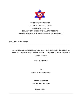
19 | P a g e
All these units and interactions between them are shown as a flowchart below:
Figure 1: Flowchart of ABC algorithm

20 | P a g e
CHAPTER III: METHODOLOGY
In this chapter, the overall procedure of performing DNR, and optimization of sizing, placement, and
operating power factor of DGs are explained.
3.1 Power Distribution System Modeling
In this work, MATPOWER toolbox of MATLAB was utilized to carry out power flow simulations of
the standard IEEE test distribution systems. The test distribution systems were modeled as power lines
and loads in MATPOWER. Initially, nbr number of branch data was supplied in nbr number of rows.
An additional oSw number of branch data for tie-lines (open branches) was fed in the next oSw number
of rows along with original branch data. Branch data included branch resistance and branch reactance.
Bus data for nbus number of buses was also fed to the computer program. Bus data included bus
number, active power load and reactive power load at the bus. It is to be noted that nbus = (nbr + 1) in
a radial network.
To demonstrate the performance and effectiveness of Artificial Bee Colony (ABC) algorithm from
small-scale to large-scale distribution networks, it has been be applied to standard IEEE test systems.
However, the computer program was designed in such a way that it can accept data of any radial
distribution network, how large or small may it be.
The developed computer program was applied to Daachhi feeder of Kathmandu. The size and GPS
location of each distribution transformer was collected along with the routing of the HT lines. All
those data were used to plot the feeder in QGIS. The line length was extracted from the QGIS. The
limitation of this approach is that the line length doesn’t consider the sag of the conductor. And, the
load power factor was taken from the substation where the feeder originated.

21 | P a g e
3.2 Short-listing of the candidate buses for installation of DGs
Voltage Stability Index (VSI) that identifies the most sensitive bus is be used to determine the
candidate bus locations for DG installation in the system, as explained in the Literature Review.
The estimation of these candidate buses initially helps in reducing the search space significantly for
the optimization technique.
A new approach of short-listing the candidate buses for installation of DGs has been applied. In
various literatures, the first ‘n’ number of buses with lowest values of VSI are directly selected for the
installation of DGs. However, that approach sidelines the opportunity to try other buses for installing
DGs. To handle that issue, computer program developed for this thesis work has been designed to
shortlist first nc number of candidate buses based on VSI values, the lowest value for nc shall not be
less than the number of DGs to be installed and the largest value for nc shall not be more than the
number of buses in the radial network. For example, ten buses can be shortlisted as candidate buses
for the installation of three DGs against only three bus as proposed in various literatures.
3.3 Cases of Analysis
Six cases of analysis have been carried out. The description of various cases is given below:
Base Case:
Evaluation of the objective function for the base case i.e. without network reconfiguration and
without insertion of DGs: The network configuration scenario for the base case has been fed into
MATLAB computer program. The base case is the condition when all the tie-lines are in open
condition. The computer program gives the base case voltage profile and base case power loss. The
improvements to be achieved in later stages of analysis has been compared with that of the base case.
Case I:
Distribution network reconfiguration of the existing network and evaluation of the objective
function for the reconfigured network: This is the first part of analysis where only the

22 | P a g e
reconfiguration has been done of the existing network by considering the given tie-lines, which were
in open condition for the base case. The computer program optimizes the voltage profile and power
loss.
Case II:
No reconfiguration of the network and performing only the insertion of DGs: In this analysis,
only the DGs are placed in the candidate buses, candidate buses being identified from VSI method.
Tie-lines are open in this stage of analysis. The computer program optimizes the size, location, and
power factor of DGs to optimize voltage profile and power loss.
Case III:
First insertion of DGs in the existing network and then performing the network reconfiguration:
This is the third case of analysis where the tie-lines are kept open and optimization of DGs parameters
is done. The shortlisting of locations for installation of DGs is done using VSI method. The computer
program gives optimum size, location and power factor of DGs. By considering the given size,
location and power factor of DGs, the computer program performs network reconfiguration. The
computer program then gives optimized voltage profile and power loss at the end of reconfiguration.
Case IV:
First reconfiguring the existing network and then performing insertion of DGs: In fourth case of
analysis, the network reconfiguration is performed where tie-lines can be switched on or off. After
finding out the best configuration, the computer program optimizes the size, location and power factor
of DGs. The shortlisting of locations for installation of DGs is done using VSI method. At the end of
the computer program, optimal voltage profile and power loss is given.
Case V:
Simultaneous reconfiguration of the network and addition of DGs: This is the last stage of analysis
and it holds the core objective of this thesis work. All the branches can be turned open or closed, along
with the tie-lines. Then, there is certain number of DGs willing to be connected in the given
distribution network. Now, the computer program performs simultaneous network reconfiguration,
and sizing & placement of DGs along with optimization of operating power factor of DGs. At the end
of the computer program, optimum configuration of the network is given along with sizing, placement

23 | P a g e
and optimal operating power factor of DGs. That solution is the best one to optimize voltage profile
and power loss.
3.4 Problem Formulation
The Objective Function for the solution is to:
3.5 Solution Variables supplied to ABC algorithm
For six cases of analysis, as explained in the section 4.3, different sets of variables were supplied to
the ABC algorithm:
Base Case:
Evaluation of the objective function for the base case i.e. without network reconfiguration and
without insertion of DGs: For the base case, no optimization had to be done. So, only the base case
voltage profile, power loss, branch currents and source power factor were calculated.
Case I:
Distribution network reconfiguration of the existing network and evaluation of the objective
function for the reconfigured network: The number of variables equaled the number of open
branches in the radial network. Those open lines are also called tie-lines or the lines out-of-service.
PR
T,Loss = Total power loss of the system after reconfiguration
PDG
T,Loss = Total power loss of the system with DGs
PT,Loss = Total power loss of the system (base case)
PLk = Real power load at bus k
PLoss(k,k+1) = Real power loss in the line connecting buses k and k+1
PDG,k = Real power supplied by DG at node k
Pss = Power supplied by the substation
Vk = Voltage magnitude at bus k
∆Vmax = Maximum voltage drop limit between buses 1 (substation) and k
Sk = Apparent power flowing in the line section between buses k and k+1
Sk,max = Maximum power flow capacity limit of line section between buses
k and k+1
Pmin
TDG = Minimum total real power generation limit
PTDG = Total real power supplied by DG in the system
Pmax
TDG = Maximum total real power generation limit
ΔVD = max{(V1-Vk)/V1} where k=1, 2,….,n

24 | P a g e
The optimal solution would be that set of open branches for which the value of objective function
would be minimum.
Case II:
No reconfiguration of the network and performing only the insertion of DGs: The number of
variables is equal to three times the number of DGs. If n is the number of DGs, then first n corresponds
to the size of DGs in MW, next n corresponds to the bus location of DGs, and the last n corresponds
to the power factor that the DGs operate. For the optimal solution, the 3n is the number of variables
corresponding to DG size, location and power factor should give the minimum value of objective
function.
Case III: First insertion of DGs in the existing network and then performing the network
reconfiguration: Firstly, the parameters related to DGs had to be optimized. So, the number of
variables would be 3n, if n is the number of DGs. Then, first n corresponds to the size of DGs in MW,
next n corresponds to the bus location of DGs, and the last n corresponds to the power factor that the
DGs operate. Secondly, the optimum configuration of the branches had to be done. So, the DG
parameters from the first part was taken and that was used while performing the reconfiguration. Here,
the number of variables was oSw, where oSw is the number of open branches. At the end of this
analysis, the best configuration of the network was found where the insertion of DGs was already
done.
Case IV:
First reconfiguring the existing network and then performing insertion of DGs: Firstly, the
reconfiguration problem had to be solved. So, the number of variables was oSw, where oSw is the
number of open branches. Now, using that configuration of the network, DGs had to be added in the
system. If n is the number of DGs, then first n corresponds to the size of DGs in MW, next n
corresponds to the bus location of DGs, and the last n corresponds to the power factor that the DGs
operate. For the optimal solution, the 3n is the number of variables corresponding to DG size, location
and power factor. At the end of the analysis, the best parameters of DGs (size, location, and power
factor) were found for the network where network reconfiguration was already done.
Case V:
Simultaneous reconfiguration of the network and addition of DGs: In this stage of analysis, the
number of variables is (oSw + 3n), where oSw is the number of open branches, and n is the number

25 | P a g e
of DGs. The first oSw number of variables give the set of open branches in the network. The next n
variables give the size of DGs, the next n variables give the location of DGs, and the last n variables
give the operating power factor of DGs. The best solution would be that set of (oSw + 3n) variables
which gives the least value of the objective function.
3.6 Steps in ABC algorithm
Initialization: The first phase in ABC is initialization of parameters (Colony Size, Limit for scout
bees, and maximum number of cycles) and set up an initial population randomly using:
where i = 1, 2, . . . , (Colonysize/2) and j = 1, 2 . . . , D. Here, D represent dimension of problem. pij
denotes location of ith
solution in jth
dimension. LBj and UBj denotes lower and upper boundary values
of search region correspondingly. rand is a randomly selected value in the range [0, 1].
Employed Bee Phase: This phase tries to detect superior quality solutions in proximity of current
solutions. If the quality of fresh solution is enhanced than present solution, the position is updated.
The position of employed bee updated using:
where φij ∈ [-1, 1] is an arbitrary number, k ∈ 1, 2, . . . (Colonysize/2) is a haphazardly identified index
such that k ≠i. In this equation, s denotes step size of position update equation. A larger step size leads
to skipping of actual solution and convergence rate may degrade if step size is very small.
Onlooker Bee Phase: The selection of a food source depends on their probability of selection. The
probability is computed using fitness of solution with the help of:
Scout Bee Phase: An employed bee become a scout bee when the solution value not updated till the
predefined threshold limit. This scout bee engenders new solution instead of rejected solution using:

26 | P a g e
Parameters of ABC algorithm:
i. Number of Population: This is an important parameter in ABC algorithm as it determines
how many solution sets are generated and tried in one iteration to optimize for the best
objective function. The Number of Population should be decided by considering the problem
dimension and the complexity of the problem. In general, it should be around 50, as a general
rule of thumb.
ii. Limit: The parameter Limit is very important in rejecting the given solution set. It signifies
how many times a given solution is given the opportunity to be better before it is rejected. For
this thesis, the value of limit was varied from 2 to 5 to find the best solution. In general, it was
observed that if limit = 2, then the solution converged very fast but sometimes it missed the
global optima. If its value was increased gradually, the number of iterations for convergence
increased but the algorithm found the global optima.
iii. Upper Bound and Lower Bound: These parameters decide the lowest bound and the highest
bound of each solution of the given solution vector. The lower bound and upper bound for the
open set of branches (for reconfiguration) was 1 and the number of branches in radial
configuration respectively. For the size of DGs, the lowest bound was 10% of the total active
power load of the network and the highest bound was 60% pf the total active power load of
the network. The lowest bound for the location of DGs was 1 and the highest bound was the
number of buses in the network. The lowest bound for the power factor of operation of DGs
was 0.7 and the highest bound was 1.
3.7 Checking Radial Topology
Radial topology was checked for all the trial solutions found by ABC algorithm. The solutions were
deemed infeasible when the solution violated any of the constraint. Prior to checking any of the
constraint, the trial solution was checked whether it maintained radial topology or not. If not, that
solution was rejected and the algorithm checked for another solution.
Step 1: Initialize a connected matrix of the loop distribution network A(b,b) with b is the number of
buses of the network system. Each entry in matrix A is defined as follows:

27 | P a g e
A(i,j) = 1 and A(j,i) = 1 if node i is connected to node j.
A(i,j) = 0 and A(j,i) = 0 if node i is not connected to node j
Initialize a set of power buses S = [feeder1, feeder2,. . .,feederk], with k is the number of feeders in the
network system.
Step 2: Read the trial solution. This is a set of tie-switches, which need to check and modify A(i,j) =
0 and A(j,i) = 0 if the switch on the branch from node i to node j is a tie-switch.
Step 3: Evaluate all load nodes as follows:
If node n R S and A(m,n) = 1, with m = 1, 2,. . .,length(S) and n = k + 1, k + 2,. . .,b then the node n
is moved to S, S = S + [node n] and A(m,n) = 0, A(n,m) = 0.
Step 4: If matrix A is a zero matrix and length of array S is equal to the number of buses then the trial
solution is a radial network configuration.
Following flowchart shows the procedure adopted to check radial topology for any set of open
branches.

28 | P a g e
Figure 2: Flowchart for checking radial topology

29 | P a g e
To fulfil the objectives of this thesis work, a computer program was developed in MATLAB using
MATPOWER toolbox. Following are the salient features of the computer program:
i. It asks the user what analysis to perform among a set of choices, as shown in figure below:
ii. It asks user whether to perform analysis on standard buses or to import custom data of any
radial network. The branch data of tie-lines shall be on the bottom rows where the branch data
lies.
Figure 3: Choices for type of analysis
Figure 4: Options to choose data set

30 | P a g e
iii. The computer program asks user for the Population Size, Number of Iterations, Parameter
Limit, Number of DGs, and number of shortlisted buses for DG installations (VSI count limit).
iv. The result of the computer program includes the optimal configuration of the network, the size,
location, and operating power factor of DGs, the voltage profile of the network (in kV and per
unit), branch currents, active power loss, reactive power loss, active/reactive power
drawn/injected into the grid, and power factor of the power drawn from the grid.
Figure 5: Windows for user inputs

31 | P a g e
Figure 6: Result format

32 | P a g e
Figure 8: Voltage Profile (numbers) format Figure 7: Branch Current format

33 | P a g e
Figure 9: Voltage Profile Comparison (Before and After) format

34 | P a g e
CHAPTER IV: SYSTEM UNDER CONSIDERATION,
SOFTWARE AND TOOLS
4.1 Systems under consideration
To examine the effectiveness of methodology proposed in this thesis work, the results were compared
with that of the reference papers for IEEE 33 Bus system, and IEEE 69 Bus system.
Each system has extra set of branches, also called tie-lines, between some buses, which are open
initially. For IEEE 33 Bus system, there are five tie-lines, and there are same number of tie-lines for
IEEE 69 Bus system.
Figure 10: IEEE 33 Bus Test System

35 | P a g e
Table 1 shows the system data for IEEE 33-Bus system.
Figure 11: IEEE 69 Bus Test System

36 | P a g e
Table 1: System data for 33-bus radial distribution network (‘*’ denotes a tie-line)
Branch
No.
Sending
Bus
Receiving
Bus
Resistance
(Ohm)
Reactance
(Ohm)
Nominal Load at Receiving
Bus
P (kW) Q (kVAR)
1 1 2 0.0922 0.047 100 60
2 2 3 0.493 0.2511 90 40
3 3 4 0.366 0.1864 120 80
4 4 5 0.3811 0.1941 60 30
5 5 6 0.819 0.707 60 20
6 6 7 0.1872 0.6188 200 100
7 7 8 0.7114 0.2351 200 100
8 8 9 1.03 0.74 60 20
9 9 10 1.044 0.74 60 20
10 10 11 0.1966 0.065 45 30
11 11 12 0.3744 0.1298 60 35
12 12 13 1.468 1.155 60 35
13 13 14 0.5416 0.7129 120 80
14 14 15 0.591 0.526 60 10
15 15 16 0.7463 0.545 60 20
16 16 17 1.289 1.721 60 20
17 17 18 0.732 0.574 90 40
18 2 19 0.164 0.1565 90 40
19 19 20 1.5042 1.3554 90 40
20 20 21 0.4095 0.4784 90 40
21 21 22 0.7089 0.9373 90 40
22 3 23 0.4512 0.3083 90 50
23 23 24 0.898 0.7091 420 200

37 | P a g e
24 24 25 0.896 0.7011 420 200
25 6 26 0.203 0.1034 60 25
26 26 27 0.2842 0.1447 60 25
27 27 28 1.059 0.9337 60 20
28 28 29 0.8042 0.7006 120 70
29 29 30 0.5075 0.2585 200 600
30 30 31 0.9744 0.963 150 70
31 31 32 0.3105 0.3619 210 100
32 32 33 0.341 0.5302 60 40
33 21 8 2.0000 2.0000 - -
34 9 15 2.0000 2.0000 - -
35 12 22 2.0000 2.0000 - -
36 18 33 0.5000 0.5000 - -
37 25 29 0.5000 0.5000 - -
Table 2 shows the system data for IEEE 69-Bus system.
Table 2: System data for 69-bus radial distribution network (‘*’ denotes a tie-line)
Branch
No.
Sending
Bus
Receiving
Bus
Resistance
(Ohm)
Reactance
(Ohm)
Nominal Load at
Receiving Bus
P (kW) Q (kVAR)
1 1 2 0.0005 0.0012 0 0
2 2 3 0.0005 0.0012 0 0
3 3 4 0.0015 0.0036 0 0
4 4 5 0.0251 0.0294 0 0
5 5 6 0.366 0.1864 2.6 2.2

38 | P a g e
6 6 7 0.3811 0.1941 40.4 30
7 7 8 0.0922 0.047 75 54
8 8 9 0.0493 0.0251 30 22
9 9 10 0.819 0.2707 28 19
10 10 11 0.1872 0.0619 145 104
11 11 12 0.7114 0.2351 145 104
12 12 13 1.03 0.34 8 5
13 13 14 1.044 0.345 8 5.5
14 14 15 1.058 0.3496 0 0
15 15 16 0.1966 0.065 45.5 30
16 16 17 0.3744 0.1238 60 35
17 17 18 0.0047 0.0016 60 35
18 18 19 0.3276 0.1083 0 0
19 19 20 0.2106 0.069 1 0.6
20 20 21 0.3416 0.1129 114 81
21 21 22 0.014 0.0046 5 3.5
22 22 23 0.1591 0.0526 0 0
23 23 24 0.3463 0.1145 28 20
24 24 25 0.7488 0.2475 0 0
25 25 26 0.3089 0.1021 14 10
26 26 27 0.1732 0.0572 14 10
27 3 28 0.0044 0.0108 26 18.6
28 28 29 0.064 0.1565 26 18.6
29 29 30 0.3978 0.1315 0 0
30 30 31 0.0702 0.0232 0 0
31 31 32 0.351 0.116 0 0
32 32 33 0.839 0.2816 14 10
33 33 34 1.708 0.5646 9.5 14
34 34 35 1.474 0.4873 6 4

39 | P a g e
35 3 36 0.0044 0.0108 26 18.55
36 36 37 0.064 0.1565 26 18.55
37 37 38 0.1053 0.123 0 0
38 38 39 0.0304 0.0355 24 17
39 39 40 0.0018 0.0021 24 17
40 40 41 0.7283 0.8509 1.2 1
41 41 42 0.31 0.3623 0 0
42 42 43 0.041 0.0478 6 4.3
43 43 44 0.0092 0.0116 0 0
44 44 45 0.1089 0.1373 39.22 26.3
45 45 46 0.0009 0.0012 39.22 26.3
46 4 47 0.0034 0.0084 0 0
47 47 48 0.0851 0.2083 79 56.4
48 48 49 0.2898 0.7091 384.7 274.5
49 49 50 0.0822 0.2011 384.7 274.5
50 8 51 0.0928 0.0473 40.5 28.3
51 51 52 0.3319 0.1114 3.6 2.7
52 52 53 0.174 0.0886 4.35 3.5
53 53 54 0.203 0.1034 26.4 19
54 54 55 0.2842 0.1447 24 17.2
55 55 56 0.2813 0.1433 0 0
56 56 57 1.59 0.5337 0 0
57 57 58 0.7837 0.263 0 0
58 58 59 0.3042 0.1006 100 72
59 59 60 0.3861 0.1172 0 0
60 60 61 0.5075 0.2585 1244 888
61 61 62 0.0974 0.0496 32 23
62 62 63 0.145 0.0738 0 0
63 63 64 0.7105 0.3619 227 162

40 | P a g e
64 64 65 1.041 0.5302 59 42
65 11 66 0.2012 0.0611 18 13
66 66 67 0.0047 0.0014 18 13
67 12 68 0.7394 0.2444 28 20
68 68 69 0.0047 0.0016 28 20
69* 11 43 0.5 0.5 - -
70* 13 21 0.5 0.5 - -
71* 15 46 1 1 - -
72* 50 59 2 2 - -
73* 27 65 1 1 - -
After proving the effectiveness of the proposed algorithm, the methodology was applied to a practical
distribution system, Daachhi feeder, of Kathmandu, Nepal. Daachhi feeder originates from Chabahil
substation situated in Chabahil, Kathmandu. The feeder is under the control of Baneshwor Distribution
Center, Nepal Electricity Authority. Required branch data, and load data was collected for the feeder
and plotted in QGIS. Bus numbers and branch numbers were assigned. Later, the data was entered in
MS-Excel in the format mentioned in Chaper III.
Figure 12 shows the GIS plot, and Table 3 has the system data for Daachhi feeder.

41 | P a g e
Figure 13 shows the single line diagram of the Daachhi feeder.
Figure 12: GIS Plot of Daachhi Feeder

42 | P a g e
Figure 13: SLD of Daachhi feeder

43 | P a g e
Table 3: System data for distribution network of Daachhi feeder of Kathmandu valley (‘*’ denotes a tie-line)
Branch
No.
Sending
Bus
Receiving
Bus
Length
(m)
Resistance
(Ohm)
Reactance Power Demand
(Ohm) P (MW)
Q
(MVAR)
1 1 2 33 0.023602 0.012754 0 0
2 2 3 30 0.021457 0.011594 0.07 0.071414
3 2 4 480 0.343307 0.185512 0 0
4 4 5 601 0.429849 0.232276 0.035 0.035707
5 5 6 780 0.557874 0.301457 0.07 0.071414
6 6 7 40 0.028609 0.015459 0.035 0.035707
7 7 8 441 0.315413 0.170439 0 0
8 8 9 97 0.069377 0.037489 0.07 0.071414
9 8 10 237 0.169508 0.091596 0.07 0.071414
10 8 11 18 0.012874 0.006957 0.14 0.142829
11 11 12 476 0.340446 0.183966 0 0
12 12 13 17 0.012159 0.00657 0.07 0.071414
13 12 14 116 0.082966 0.044832 0 0
14 14 15 19 0.013589 0.007343 0.07 0.071414
15 14 16 91 0.065085 0.03517 0.14 0.142829
16 16 17 47 0.033615 0.018165 0.07 0.071414
17 16 18 27 0.019311 0.010435 0.14 0.142829
18 18 19 45 0.032185 0.017392 0.21 0.214243
19 4 20 80 0.057218 0.030919 0.07 0.071414
20 20 21 290 0.207415 0.11208 0.07 0.071414
21 21 22 100 0.071522 0.038648 0.21 0.214243
22 22 23 84 0.060079 0.032465 0.14 0.142829
23 23 24 370 0.264633 0.142999 0.07 0.071414

44 | P a g e
24 24 25 390 0.278937 0.150728 0.112 0.114263
25 22 26 189 0.135177 0.073045 0 0
26 26 27 119 0.085112 0.045991 0.105 0.107121
27 26 28 77 0.055072 0.029759 0 0
28 28 29 17 0.012159 0.00657 0.07 0.071414
29 28 30 663 0.474193 0.256238 0.07 0.071414
30 30 31 448 0.32042 0.173144 0.035 0.035707
31 31 32 182 0.130171 0.07034 0.07 0.071414
32 26 33 183 0.130886 0.070726 0 0
33 33 34 45 0.032185 0.017392 0.21 0.214243
34 34 35 598 0.427703 0.231117 0.07 0.071414
35 35 36 342 0.244606 0.132177 0.14 0.142829
36 36 37 73 0.052211 0.028213 0.07 0.071414
37 37 38 419 0.299678 0.161936 0.035 0.035707
38 38 39 235 0.168077 0.090823 0.035 0.035707
39 39 40 408 0.291811 0.157685 0.07 0.071414
40 33 41 52 0.037192 0.020097 0.035 0.035707
41 41 42 63 0.045059 0.024348 0.07 0.071414
42 42 43 86 0.061509 0.033238 0 0
43 43 44 65 0.04649 0.025121 0.2205 0.224955
44 43 45 223 0.159495 0.086186 0.14 0.142829
45 45 46 30 0.021457 0.011594 0 0
46 46 47 94 0.067231 0.036329 0 0
47 47 48 79 0.056503 0.030532 0.14 0.142829
48 47 49 267 0.190965 0.103191 0.14 0.142829
49 49 50 54 0.038622 0.02087 0.0175 0.017854
50 46 51 223 0.159495 0.086186 0.07 0.071414
51 51 52 830 0.593635 0.320781 0.14 0.142829
52 52 53 148 0.105853 0.057199 0.07 0.071414

45 | P a g e
53* 10 17 382 0.273215 0.147636 - -
54* 5 25 484 0.346168 0.187058 - -
55* 50 53 595 0.425558 0.229957 - -
56* 27 44 65 0.04649 0.025121 - -
57* 32 40 610 0.436286 0.235755 - -
4.2 Software and Tools Used
MATLAB’s programming environment was the software used in this thesis. MATLAB stands for
"Matrix Laboratory" is a proprietary multi-paradigm programming language and numerical computing
environment developed by MathWorks. MATLAB allows matrix manipulations, plotting of functions
and data, implementation of algorithms, creation of user interfaces, and interfacing with programs
written in other languages. Common usage of the MATLAB application involves using the "Command
Window" as an interactive mathematical shell or executing text files containing MATLAB code.
As this thesis work involves numerous power flow computations in one iteration, a time-efficient way
to compute power flow results is required. MATPOWER is a package of MATLAB M-files for
solving power flow and optimal power flow problems. It is intended as a simulation tool for
researchers and educators that is easy to use and modify. MATPOWER is designed to give the best
performance possible while keeping the code simple to understand and modify. MATPOWER was
initially developed by Ray D. Zimmerman, Carlos E. MurilloS´anchez and Deqiang Gan at Cornell
University under the direction of Robert J. Thomas.

46 | P a g e
CHAPTER V: RESULTS AND DISCUSSIONS
This chapter presents the results achieved in this thesis work. Firstly, the results were first compared
against those in the reference paper [13]. In various literatures related to distribution network
reconfiguration and installation of DGs, provision of specifying the nature of DGs have not been
considered. In those works, the DGs were assumed to have injected active power only i.e. operating
at unity power factor. In practice, there are following types of DGs:
o DGs injecting active power only,
o DGs injecting both active and reactive power,
o DGs injecting active power but absorbing reactive power.
This thesis work has taken the incorporation of DGs in the given distribution network one notch further
and studies the effect of having different types of DGs. Taking that improvement into consideration,
the developed computer program was run with exactly same inputs as in the reference paper 13 except
specifying that one of the DGs injects active power only, another one injecting both active power and
reactive power, and the last DG injecting active power but absorbing reactive power. The lower limit
of power factor was taken to be 0.8.
5.1 For IEEE 33 Bus System
Base Case: For the base case, the result for the power loss achieved in this thesis work (202.67 kW)
is exactly same with what given in reference paper 13. It shows that the network parameters
considered in both scenarios are exactly same.
Case I: For the network reconfiguration only case, the configuration for the network recommended
in the reference paper 13 exactly matches with that achieved in this thesis work (7-14-9-32-28).
Hence, the power loss (139.978 kW) and minimum voltage (0.913 pu at 18th
bus) match in both the
cases. Until this case, there is not much significance on the choice of optimization algorithm.
Case II: For the DG Installation only case, the results achieved in this thesis work using ABC
algorithm is superior to that given in the reference paper 13. The power loss and min. bus voltage
achieved in this thesis work is 82.769 kW and 0.9413 pu (32nd
bus) against 88.68 kW and 0.968 pu
(30th
bus) in the reference paper 13. All the DGs were considered to inject active power only. When

47 | P a g e
DGs were considered to inject both active power and reactive power (pf limited to 0.8 lagging), the
power loss and min. bus voltage achieved in this thesis work is 26.639 kW and 0.966 pu (33rd
bus).
Case III: For the DG installation after network reconfiguration case, the results achieved in this thesis
work using ABC algorithm is superior to that given in the reference paper 13. The power loss and
min. bus voltage achieved in this thesis work is 58.283 kW and 0.976 pu (31st
bus) against 83.91 kW
and 0.9612 pu (30th
bus) in the reference paper 13. All the DGs were considered to inject active power
only. When DGs were considered to inject both active power and reactive power (pf limited to 0.8
lagging), the power loss and min. bus voltage achieved in this thesis work is 21.704 kW and 0.989 pu
(31st
bus).
Case IV: For the network reconfiguration after DG installation case, the results achieved in this thesis
min. bus voltage achieved in this thesis work is 63.217 kW and 0.975 pu (22nd
and 0.9712 pu (29th bus) in the reference paper 13. All the DGs were considered to inject active power
(18th
bus).
Case V: For the simultaneous network reconfiguration and DG installation case, the results achieved
in this thesis work using ABC algorithm is superior to that given in the reference paper 13. The power
loss and min. bus voltage achieved in this thesis work is 57.776 kW and 0.974 pu (33rd
bus) against
67.11 kW and 0.9713 pu (14th
bus) in the reference paper 13. All the DGs were considered to inject
active power only. When DGs were considered to inject both active power and reactive power (pf
limited to 0.8 lagging), the power loss and min. bus voltage achieved in this thesis work is 14.324 kW
and 0.994 pu (12th
bus).
Following table summarizes and compares the results for IEEE 33 Bus System:

48 | P a g e
Table 4: Results comparison for IEEE 33 Bus System
For IEEE 33 Bus
Using FWA [13], DGs inject
P only
Results found, DGs inject P
only
Results found, DGs inject
both P and Q
Base Case (no reconfiguration and no inclusion of DGs)
Open Branches 33-34-35-36-37 33-34-35-36-37 33-34-35-36-37
Vmin (pu) 0.913 (18) 0.913 (18) 0.913 (18)
Ploss (kW) 202.67 202.67 202.67
Only Reconfiguration (Case I), independent of presence of DGs
Open Branches 7-14-9-32-28 7-14-9-32-28
Vmin (pu) 0.941 (32) 0.941 (32)
Ploss (kW) 139.98 (less by 30.93%) 139.98 (less by 30.93%)
Only DG Installation (Case II)
Open Branches 33-34-35-36-37 33-34-35-36-37 33-34-35-36-37
Vmin (pu) 0.968 (30) 0.951 (33) 0.966 (33)
Ploss (kW) 88.68 (less by 56.24%) 82.77 (less by 59.16%) 26.64 (less by 86.86%)
DG cap. (MW),
loc., and
operating pf
0.590 (14), 0.190 (18),
1.010 (32)
0.677 (31), 1.629 (26),
0.817 (25)
1.132 (30) at 0.800 pf,
0.890 (25) at 0.902 pf,
1.645 (26) at 0.822 pf
DG Installation after Reconfiguration (Case III)
Open Branches 7-14-9-32-28 7-14-9-32-28 7-14-9-32-28
Vmin (pu) 0.961 (30) 0.976 (31) 0.989 (31)
Ploss (kW) 83.91(less by 58.60%) 58.28 (less by 71.24%) 21.70 (less by 89.29%)
DG cap. (MW),
loc., and
operating pf
0.600 (32), 0.310 (33),
0.160 (18)
1.551 (29), 0.509 (17),
1.454 (10)
0.639 (13) at 0.923 pf,
2.030 (25) at 0.839 pf,
0.610 (16) at 0.973 pf
Reconfiguration after DG Installation (Case IV)
Open Branches 7-34-9-32-28 30-11-14-33-28 15-33-3-13-37
Vmin (pu) 0.971 (29) 0.975 (22) 0.993 (18)
DG cap. (MW),
loc., and
operating pf
0.590 (14), 0.190 (18),
1.020 (32)
1.010 (24), 0.673 (31),
1.583 (26)
1.132 (30) at 0.800 pf,
0.890 (25) at 0.902 pf,
1.645 (26) at 0.822 pf
Simultaneous Reconfiguration & DG Installation (Case V)
Open Branches 7-14-11-32-28 9-28-17-33-34 12-8-33-28-36

49 | P a g e
For IEEE 33 Bus
P only
only
both P and Q
Vmin (pu) 0.971 (14) 0.974 (33) 0.994 (12)
DG cap. (MW),
loc., and
operating pf
0.54 (32), 0.62 (29), 0.53
(18)
0.599 (13), 0.885 (26),
1.512 (30)
0.744 (13) at 0.896 pf,
0.913 (26) at 0.887 pf,
1.736 (30) at 0.800 pf
5.2 For IEEE 69 Bus System
Base Case: For the base case, the result for the power loss achieved in this thesis work (225 kW) is
exactly same with what given in reference paper 13. It shows that the network parameters considered
in both scenarios are exactly same.
Case I: For the network reconfiguration only case, the configuration for the network recommended
in the reference paper 13 exactly matches with that achieved in this thesis work (69-70-14-56-61).
Hence, the power loss (98.611 kW) and minimum voltage (0.949 pu at 61st
bus) match in both the
cases. Until this case, there is not much significance on the choice of optimization algorithm.
Case II: For the DG Installation only case, the results achieved in this thesis work using ABC
algorithm is superior to that given in the reference paper 13. The power loss and min. bus voltage
achieved in this thesis work is 74.404 kW and 0.981 pu (64th
bus) against 77.85 kW and 0.974 pu
(62nd
bus) in the reference paper 13. All the DGs were considered to inject active power only. All the
DGs were considered to inject active power only. When DGs were considered to inject both active
power and reactive power (pf limited to 0.8 lagging), the power loss and min. bus voltage achieved in
this thesis work is 10.892 kW and 0.987 pu (69th
bus).
Case III: For the DG installation after network reconfiguration case, the results achieved in this thesis
min. bus voltage achieved in this thesis work is 37.772 kW and 0.984 pu (40th
and 0.972 pu (61st

50 | P a g e
(69th
bus).
Case IV: For the network reconfiguration after DG installation case, the results achieved in this thesis
min. bus voltage achieved in this thesis work is 42.92 kW and 0.978 pu (55th
and 0.9763 pu (61st
(64th
bus).
Case V: For the simultaneous network reconfiguration and DG installation case, the results achieved
in this thesis work using ABC algorithm is superior to that given in the reference paper 13. The power
loss and min. bus voltage achieved in this thesis work is 37.075 kW and 0.981 pu (65th
bus) against
39.25 kW and 0.98 pu (61st
bus) in the reference paper 13. All the DGs were considered to inject
active power only. When DGs were considered to inject both active power and reactive power (pf
limited to 0.8 lagging), the power loss and min. bus voltage achieved in this thesis work is 5.74 kW
and 0.995 pu (57th
bus).
Following table summarizes and compares the results for IEEE 69 bus system:
Table 5: Results comparison for IEEE 69 Bus System
For IEEE 69 Bus
P only
only
both P and Q
Base Case (no reconfiguration and no inclusion of DGs)
Open Branches 69-70-71-72-74 69-70-71-72-73 69-70-71-72-73
Vmin (pu) 0.913 (18) 0.913 (18) 0.913 (18)
Ploss (kW) 225 225 225
Only Reconfiguration (Case I), independent of presence of DGs
Open Branches 69-70-14-56-61 69-14-61-56-70
Vmin (pu) 0.950 (61) 0.950 (61)
Ploss (kW) 98.60 (less by 56.18%) 98.61 (less by 56.17%)
Only DG Installation (Case II)

Thesis Report.pdf

Recommended

Recommended

More Related Content

Similar to Thesis Report.pdf

Similar to Thesis Report.pdf (20)

Recently uploaded

Recently uploaded (20)

Thesis Report.pdf