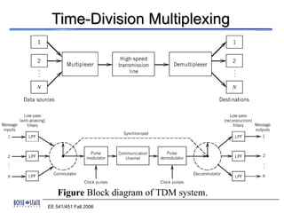
Pulse code modulation (PCM) is an analog-to-digital conversion technique used to represent sampled analog signals as digital data. PCM involves sampling the analog signal at regular intervals, quantizing the amplitude of the signal at each point to a few discrete levels, and coding it as digital data. The sampling rate must be greater than twice the highest frequency of the analog signal as per the Nyquist sampling theorem. PCM was invented in 1937 but was not widely adopted until the 1940s. It became the standard method for digital telephony due to its robustness and ability to efficiently regenerate and transmit signals.

1. Pulse Code Modulation (PCM)
 Pulse code modulation (PCM) is produced by analog-to-digital conversion
process. Quantized PAM
 As in the case of other pulse modulation techniques, the rate at which
samples are taken and encoded must conform to the Nyquist sampling rate.
 The sampling rate must be greater than, twice the highest frequency in the
analog signal,
fs > 2fA(max)
 Telegraph time-division multiplex (TDM) was conveyed as early as 1853, by
the American inventor M.B. Farmer. The electrical engineer W.M. Miner, in
1903.
 PCM was invented by the British engineer Alec Reeves in 1937 in France.
 It was not until about the middle of 1943 that the Bell Labs people became
aware of the use of PCM binary coding as already proposed by Alec Reeves.
EE 541/451 Fall 2006

2. Pulse Code Modulation
Figure The basic elements of a PCM system.
EE 541/451 Fall 2006

3. Encoding
EE 541/451 Fall 2006

4. Virtues, Limitations and Modifications of PCM
Advantages of PCM
1. Robustness to noise and interference
2. Efficient regeneration
3. Efficient SNR and bandwidth trade-off
4. Uniform format
5. Ease add and drop
6. Secure
DS0: a basic digital signaling rate of 64 kbit/s. To carry a typical
phone call, the audio sound is digitized at an 8 kHz sample rate
using 8-bit pulse-code modulation. 4K baseband, 8*6+1.8 dB
EE 541/451 Fall 2006

5. Two Types of Errors
 Round off error
 Detection error
 Variance of sum of the independent random variables is equal to
the sum of the variances of the independent random variables.
 The final error energy is equal to the sum of error energy for
two types of errors (12.56-12.59)
 Round off error in PCM
– Example 10.17 Page 467
2
1  mp 
σ = 
2
q  L 
3 
EE 541/451 Fall 2006

6. Mean Square Error in PCM
 If transmit 1101 (13), but receive 0101 (5), error is 8
 Error in different location produces different MSE
ε i = (2 − i )(2m p )
 Overall error probability
– Page 469
n n 4m 2 Pe (2 2 n − 1)
MSE = ∑ ε i2 Pe (ε i ) = Pe ∑ ε i2 =
p
i =1 i =1 3(2 2 n )
– Gray coding: if one bit occur, the error is minimized.
EE 541/451 Fall 2006

7. Bit Errors in PCM Systems
Simplest case is Additive
White Gaussian Noise for
baseband PCM scheme --
see the analysis for this
case. For signal levels of
+A and -A we get
pe = Q(A/σ)
Notes
•Q(A/σ) represents the area under one tail of the normal pdf
•(A/σ)2 represents the Signal to Noise (SNR) ratio
• Our analysis has neglected the effects of transmit and receive filters - it
can be shown that the same results apply when filters with the correct
response are used.
EE 541/451 Fall 2006

8. Q Function
 For Q function: 10
0
– The remain of cdf of Gaussian
distribution
-2
10
– Physical meaning
– Equation
( )
-4
10
Pe = Q γ
-6
10
 Matlab: erfc Q F u n c tio n
– y = Q(x)
– y = 0.5*erfc(x/sqrt(2));
-8
10
 Note how rapidly Q(x) decreases
as x increases - this leads to the 10
-1 0
0 1 2 3 4 5 6
threshold characteristic of digital
communication systems
EE 541/451 Fall 2006

9. SNR vs. γ
 Figure 12.14: Exam, Exam and Exam
S0  m2 
3(2 2 n )
=  
N 0 1 + 4(2 − 1)Q( γ / n0 )  m p 
2n

2 
 Threshold
 Saturation
– Equation 12.64C, slightly better than ADC
 Example 12.8
 Exchange of SNR for bandwidth is much more efficient
than in angle modulation
 Repeaters
EE 541/451 Fall 2006

10. Companded PCM
 m2 
 Problem of  
 m2 
 p
 Without compand, 12.67
 With compand, 12.68
 Final SNR 12.72b
 Saturation 12.72C
 Small input signal 12.73
 Figure 12.17 for µ law
– Even the input signal is very small, the output SNR is still
reasonable.
EE 541/451 Fall 2006

11. Optimal Pre-emphasis and De-emphasis
 System model: Figure 12.18
 Distortion-less condition
– 12.76a for amplitude and 12.76b for phase
 SNR expression 12.78
 Maximize SNR s.t. distortionless
 Lagrange multiplier
 Optimal Hp and Hd, 12.83a and 12.83b
 SNR improvement, 12.83c
 Example 12.11
EE 541/451 Fall 2006

12. Pre-emphasis and De-emphasis in AM and FM
 AM
– No that effective
 FM
– Noise is larger when frequency is high
– Optimal pre-emphasis and de-emphasis, 12.88d
– Only simple suboptimum is used in commercial FM for historical
and practical reasons
EE 541/451 Fall 2006

13. Differential Encoding
 Encode information in terms of signal transition; a
transition is used to designate Symbol 0
Regeneration (reamplification, retiming, reshaping )
3dB performance loss, easier decoder
EE 541/451 Fall 2006

14. Linear Prediction Coding (LPC)
Consider a finite-duration impulse response (FIR)
discrete-time filter which consists of three blocks :
1. Set of p ( p: prediction order) unit-delay elements (z-1)
2. Set of multipliers with coefficients w1,w2,…wp
3. Set of adders ( ∑ )
EE 541/451 Fall 2006

15. Reduce the sampling rate
Block diagram illustrating the linear adaptive prediction process.
EE 541/451 Fall 2006

16. Differential Pulse-Code Modulation (DPCM)
Usually PCM has the sampling rate higher than the Nyquist rate.
The encode signal contains redundant information. DPCM can efficiently
remove this redundancy. 32 Kbps for PCM Quality
EE 541/451 Fall 2006

17. Processing Gain
The (SNR) o of the DPCM system is
σM
2
(SNR) o = 2
σQ
where σ M and σ Q are variances of m[ n] ( E[m[n]] = 0) and q[ n]
2 2
σM σE
2 2
(SNR) o = ( 2 )( 2 )
σ E σQ
= G p (SNR )Q
where σ E is the variance of the predictions error
2
and the signal - to - quantization noise ratio is
σE
2
(SNR ) Q = 2
σQ
σM
2
Processing Gain, G p = 2
σE
Design a prediction filter to maximize G p (minimize σ E )
2
EE 541/451 Fall 2006

18. Adaptive Differential Pulse-Code Modulation (ADPCM)
Need for coding speech at low bit rates , we have two aims in mind:
1. Remove redundancies from the speech signal as far as possible.
2. Assign the available bits in a perceptually efficient manner.
Adaptive quantization with backward estimation (AQB).
EE 541/451 Fall 2006

19. ADPCM
8-16 kbps with the same quality of PCM
Adaptive prediction with backward estimation (APB).
EE 541/451 Fall 2006

20. Coded Excited Linear Prediction (CELP)
 Currently the most widely used speech coding algorithm
 Code books
 Vector Quantization
 <8kbps
 Compared to CD
44.1 k sampling
16 bits quantization
705.6 kbps
100 times difference
EE 541/451 Fall 2006

21. Time-Division Multiplexing
Figure Block diagram of TDM system.
EE 541/451 Fall 2006

22. DS1/T1/E1
 Digital signal 1 (DS1, also known as T1) is a T-carrier signaling
scheme devised by Bell Labs. DS1 is a widely used standard in
telecommunications in North America and Japan to transmit voice and
data between devices. E1 is used in place of T1 outside of North
America and Japan. Technically, DS1 is the transmission protocol
used over a physical T1 line; however, the terms "DS1" and "T1" are
often used interchangeably.
 A DS1 circuit is made up of twenty-four DS0
 DS1: (8 bits/channel * 24 channels/frame + 1 framing bit) * 8000
frames/s = 1.544 Mbit/s
 A E1 is made up of 32 DS0
 The line data rate is 2.048 Mbit/s which is split into 32 time slots,
each being allocated 8 bits in turn. Thus each time slot sends and
receives an 8-bit sample 8000 times per second (8 x 8000 x 32 =
2,048,000). 2.048Mbit/s
 History page 274
EE 541/451 Fall 2006

23. Synchronization
 Super Frame
EE 541/451 Fall 2006

24. Synchronization
 Extended Super Frame
EE 541/451 Fall 2006

25. T Carrier System
Twisted Wire to Cable System
EE 541/451 Fall 2006

26. Fiber Communication
EE 541/451 Fall 2006

27. Delta Modulation (DM)
Let m[ n] = m(nTs ) , n = 0,±1,±2, 
where Ts is the sampling period and m(nTs ) is a sample of m(t ).
The error signal is
e[ n] = m[ n] − mq [ n − 1]
eq [ n] = ∆ sgn(e[ n] )
mq [ n] = mq [ n − 1] + eq [ n]
where mq [ n] is the quantizer output , eq [ n] is
the quantized version of e[ n] , and ∆ is the step size
EE 541/451 Fall 2006

28. DM System: Transmitter and Receiver.
EE 541/451 Fall 2006

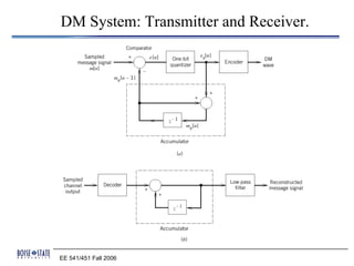
29. Slope overload distortion and granular noise
The modulator consists of a comparator, a quantizer, and an
accumulator. The output of the accumulator is
n
mq [ n] = ∆ ∑ sgn(e[ i ])
i =1
n
= ∑ eq [ i ]
i =1
EE 541/451 Fall 2006

30. Slope Overload Distortion and Granular Noise
Denote the quantization error by q[ n] ,
mq [ n] = m[ n] − q[ n]
We have
e[ n] = m[ n] − m[ n − 1] − q[ n − 1]
Except for q[ n − 1], the quantizer input is a first
backward difference of the input signal ( differentiator )
To avoid slope - overload distortion , we require
∆ dm(t )
(slope) ≥ max
Ts dt
On the other hand, granular noise occurs when step size
∆ is too large relative to the local slope of m(t ).
EE 541/451 Fall 2006

31. Delta-Sigma modulation (sigma-delta modulation)
The ∆ − Σ modulation which has an integrator can
relieve the draw back of delta modulation (differentiator)
Beneficial effects of using integrator:
1. Pre-emphasize the low-frequency content
2. Increase correlation between adjacent samples
(reduce the variance of the error signal at the quantizer input )
3. Simplify receiver design
Because the transmitter has an integrator , the receiver
consists simply of a low-pass filter.
(The differentiator in the conventional DM receiver is cancelled by
the integrator )
EE 541/451 Fall 2006

32. delta-sigma modulation system.
EE 541/451 Fall 2006

33. Adaptive Delta Modulation
 Adaptive adjust the step size according to frequency, figure 6.21
 Out SNR
– Page 286-287
– For single integration case, (BT/B)^3
– For double integration case, (BT/B)^5
 Comparison with PCM, figure 6.22
– Low quality has the advantages.
– Used in walky-talky
EE 541/451 Fall 2006