Download to read offline


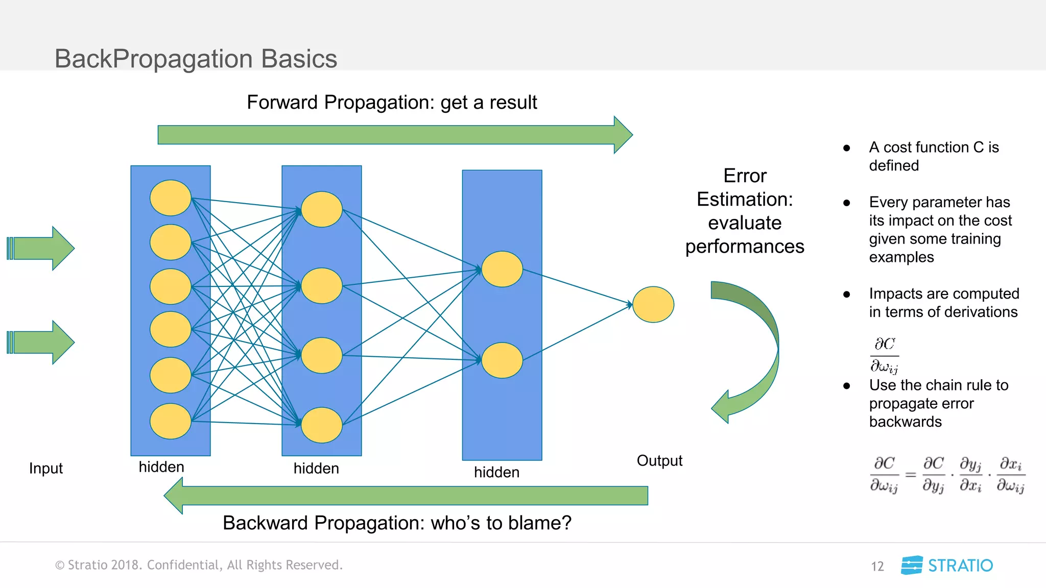


This document discusses various concepts related to convolutional neural networks (CNNs) and generative models, including backpropagation, data augmentation, and the structure of autoencoders. It covers technical details such as cost functions, activation functions, and the mechanics of training models, as well as introduces generative adversarial networks (GANs) and their applications. The text emphasizes the importance of data and the complexities of model training, alongside practical applications and insights into effective data augmentation techniques.


![[Strata] Sparkta](https://cdn.slidesharecdn.com/ss_thumbnails/stratasparktav3-150507092440-lva1-app6891-thumbnail.jpg?width=640&height=640&fit=bounds)


