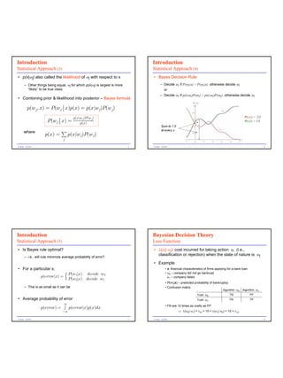
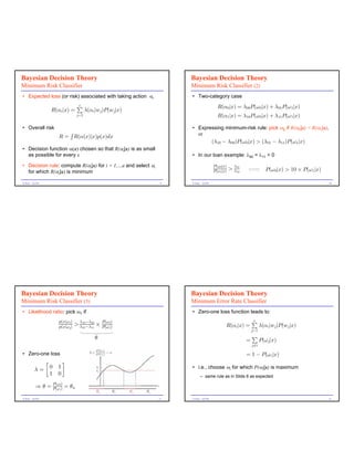
1) The document introduces Bayesian decision theory and its use for statistical pattern classification. 2) It discusses key concepts such as prior and conditional probabilities, loss functions, and deriving the minimum-risk classifier that minimizes expected loss. 3) The minimum-risk classifier chooses the decision or action that minimizes the total risk, calculated from the loss incurred for each state of nature weighted by its posterior probability.

1. Overview
• Basic statistical concepts
Introduction to Pattern Recognition and Data Mining
– Apriori probability, class-conditional density
– Bayes formula & decision rule
Lecture 2: Bayesian Decision Theory – Loss function & minimum-risk classifier
Instructor: Dr. Giovanni Seni • Discriminant functions
• Decision regions/boundaries
Department of Computer Engineering
• The Normal density
Santa Clara University – Discriminant functions (LDA)
G.Seni – Q1/04 2
Introduction Introduction
Statistical Approach Statistical Approach (2)
• A formalization of common-sense procedures… • Best decision rule about next fish type before it actually
appears?
• Quantify tradeoffs between various classification decisions
using probability – Decide ω1 if P(ω1) > P(ω2); otherwise decide ω2
– How well it works?
• Initially assume all relevant probability values are known
• P(error) = min [P(ω1), P(ω2)]
• State of nature
– What fish type (ω) will come out next? • Incorporating lightness/length info
• ω1 = salmon, ω2 = sea bass
– Class-conditional probability density
– ω is unpredictable – i.e., a random variable
p(x|ω1) and p(x|ω2) describe the difference
• A priori probability -- prior knowledge of how likely each in lightness between populations of sea bass
and salmon
fish type is -- P(ω1) + P( ω2) = 1
G.Seni – Q1/04 3 G.Seni – Q1/04 4

2. Introduction Introduction
Statistical Approach (3) Statistical Approach (4)
• p(x|ωj) also called the likelihood of ωj with respect to x • Bayes Decision Rule
– Other things being equal, ωj for which p(x|ωj) is largest is more – Decide ω1 if P(ω1|x) > P(ω2|x); otherwise decide ω2
“likely” to be true class or
– Decide ω1 if p(x|ω1)P(ω1) > p(x|ω2)P(ω2); otherwise decide ω2
• Combining prior & likelihood into posterior – Bayes formula

p(w j, x) = P(w jx)p(x) = p(x|w j)P(w j)
 p(x|w j)P(w j) P(ω1) = 2/3
P(w jx) = p(x)
P(ω2) = 1/3
Sum to 1.0
where P at every x
p(x) = p(x|w j)P(w j)
j
G.Seni – Q1/04 5 G.Seni – Q1/04 6
Introduction Bayesian Decision Theory
Statistical Approach (5) Loss Function
• Is Bayes rule optimal? • λ(αi| ωj): cost incurred for taking action αi (i.e.,
classification or rejection) when the state of nature is ωj
– i.e., will rule minimize average probability of error?
• Example
• For a particular x, • x: financial characteristics of firms applying for a bank loan
n • ω0 – company did not go bankrupt
P(w 1|x) decide w 2
p(error|x) = ω1 – company failed
P(w 2|x) decide w 1
• P(ωi|x) – predicted probability of bankruptcy
– This is as small as it can be • Confusion matrix:
Algorithm: ω0 Algorithm: ω1
Truth: ω0 TN FP
• Average probability of error Truth: ω1 FN TP
∞
• FN are 10 times as costly as FP
p(error) = ∫ p(error|x)p(x)dx
à∞ ⇒ λ(α0| ω1) = λ01 = 10 × λ(α1| ω0) = 10 × λ10
G.Seni – Q1/04 7 G.Seni – Q1/04 8

3. Bayesian Decision Theory Bayesian Decision Theory
Minimum Risk Classifier Minimum Risk Classifier (2)
• Expected loss (or risk) associated with taking action αi • Two-category case
P
c
R(ë0|x) = õ00P(ω0|x) + õ01P(ω1|x)
R(ëi|x) = õ(ëi|w j)P(w j|x)
j=1 R(ë1|x) = õ10P(ω0|x) + õ11P(ω 1|x)
• Overall risk • Expressing minimum-risk rule: pick ωo if R(α0|x) < R(α1|x),
R or
R = R(ë(x)|x)p(x)dx
(õ10 à õ00)P(ω 0|x) > (õ01 à õ11)P(ω 1|x)
• Decision function α(x) chosen so that R(αi|x) is as small
as possible for every x • In our loan example: λ00 = λ11 = 0
• Decision rule: compute R(αi|x) for i = 1,…a and select αi P(ω0|x)
> õ01 P(ω0|x) > 10 â P(ω1|x)
for which R(αi|x) is minimum P(ω1|x) õ10
G.Seni – Q1/04 9 G.Seni – Q1/04 10
Bayesian Decision Theory Bayesian Decision Theory
Minimum Risk Classifier (3) Minimum Error Rate Classifier
• Likelihood ratio: pick ω1 if • Zero-one loss function leads to:
p(x|ω1) P
c
p(x|ω2)
> õ12àõ22 â P(ω2)
õ21àõ11 P(ω1) R(ëi|x) = õ(ëi|w j)P(w j|x)
j=1
θ P
= P(ω j|x)
j6=i
• Zero-one loss 0≤ <∞
= 1 à P(ωi|x)
ô õ
õ= 0 1 • i.e., choose ωi for which P(ωi|x) is maximum
1 0 – same rule as in Slide 6 as expected
P(ω )
⇒ ò = P(ω2) = ò a
1
G.Seni – Q1/04 11 G.Seni – Q1/04 12

4. Bayesian Decision Theory Bayesian Decision Theory
Discriminant Function Discriminant Function (2)
• A useful way of representing a classifier • Two-category case – dichotomizer
– One function gi(x) for each class – A single function suffices:
– Assign x to ωi if gi(x) > gj(x) for all j≠ i
g(x) = g1(x) – g2(x)
• Minimum risk: gi(x) = - R(αi|x) – Decision rule:
Choose ω1 if g(x) > 0; otherwise choose ω2
• Minimum error: gi(x) = P(ωi|x)
– Monotonic increasing transformations are equivalent – Convenient forms
gi(x) = p(x|ωi)P(ωi) g(x) = P(ω1|x) - P(ω2|x)
gi(x) = ln p(x|ωi) + ln P(ωi) p(x|ω1) P(ω1)
g(x) = ln ______ + ln ______
p(x|ω2) P(ω2)
G.Seni – Q1/04 13 G.Seni – Q1/04 14
Bayesian Decision Theory Normal Density
Decision Regions & Boundaries Introduction
• Ri region in feature space where gi(x) > gj(x) for all j≠ i • Used to model p(x|ωi)
– Might not be simply connected
0.4
• Decision boundary: surfaces in feature space where ties 0.35
occur among largest disciminant functions
0.3
⇒
0.25
0.2
0.15
0.1
0.05
0
0 1 2 3 4 5 6 7 8
• Special attention due to:
– Analytically tractable
– A continuous-valued feature x can be seen as randomly corrupted
version of a single typical µ (asymptotically Gaussian)
G.Seni – Q1/04 15 G.Seni – Q1/04 16

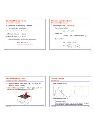
5. Normal Density Normal Density
Univariate Case Bivariate Case
• x ∼ N(0, 1) -- x is normally distributed with zero mean and • If x ∼ N(0, 1) and y ∼ N(0, 1) are independent
unit variance 0.4
1 2 2
1 2 p(x, y) = p(x) â p(y) = 2ùe à2(x +y )
1
px(x) = √1 eà2x
2ù
0.3
0.2
0 = ö = ε[x] • Contours: p(x, y) = c1 ⇒ x2 + y 2 = c2
0.1
2 2
1 = û = ε[(x à ö) ] 0 0.14
-4 -3 -2 -1 0 1 2 3 4 0.12
68% 0.1
95% 0.08
0.06
• Location-scale shift 99.7%
0.04
0.02
z=σx+µ 0
1 zàö 2 4
∼ N(µ, σ) pz(z) = √2ùûe à2(
1 û
)
= û px(zàö)
1
û -4 0
1
2
3
-3 -2 -1
-1 0 -2
1 -3
2 3 -4
4
G.Seni – Q1/04 17 G.Seni – Q1/04 18
Normal Density Normal Density
Bivariate Case (2) Multivariate Case
• If x ∼ N(µx, σx) and y ∼ N(µy, σy) are independent • We say x ∼ N(µ, Σ)
2 2
1  x−µ x  1  x−µ y 
−   −   1
1 (xàö) tΣà1(xàö)
2 σ x  2 σ y 
p(x) = (2ù)d/2|Σ| 1/2 e à2
 1

p ( x, y ) = e  
2πσ xσ y
• Contours: 1
û x2
(x à öx)2 + û12(y à öy)2 = c where,
y
ô õ ô 2 õ x = (x1, x2, …, xd)t (t stands for the transpose vector form)
0.16
ö û 0
p(x, y) = N( x , x
0.14
0.12 2 )
0.1
0.08
öy 0 ûy µ = (µ1, µ2, …, µd mean vector
)t
0.06
0.04 ô õô 2 õ
0.02
1 , 2 0 ) Σ = d× d covariance matrix
0
= N( 2
5 3 0 1 -1
3
4 2
|Σ| and Σ are determinant and inverse respectively
-4 -3 -2 -1 2
(x - µ)tΣ (x - µ) is (square) Mahalanobis distance
0 1
1 2 3 variance-covariance matrix -1
4 5 0
G.Seni – Q1/04 19 G.Seni – Q1/04 20

6. Bayesian Decision Theory Bayesian Decision Theory
Discriminant Function – Normal Density Discriminant Function – Normal Density (2)
• p(x|ωi) ∼ N(µi, Σi) • Case 1: features are statistically independent (σij= 0) and
 share same variance σ2
• We had gi(x) = ln p(xω i) + ln P(ω i)
kxàö ik 2
gi(x) = à 2û 2 + ln P(ωi)
⇒ gi(x) = à 1(x à öi)tΣà1(x à öi) à d ln 2ù
2 i 2 1
= à 2û 2[x tx à 2ötx + ötöi] + ln P(ω i)
i i
1
− ln Σ i + ln P (ωi )
2 = w tx + w i0
i
2
• Case 1: Σi = û I
1
linear discriminant function where w i = û2öi
• Case 2: Σi = Σ 1
w i0 = à 2û2[ötöi] + ln P(ωi)
i
• Case 3: Σi = arbitrary
• All priors equal ⇒ Minimum (Euclidean) distance classifier
G.Seni – Q1/04 21 G.Seni – Q1/04 22
Bayesian Decision Theory Bayesian Decision Theory
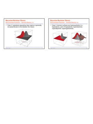
Discriminant Function – Normal Density (3) Discriminant Function – Normal Density (4)
• Case 1: distributions are “spherical” in d dimensions; • Case 2: samples fall in hyperellipsoidal clusters of equal
boundary is a hyperplane in d-1 dimensions perpendicular size and shape
to line between means
gi(x) = à 1(x à öi)tΣ à1(x à öi) + ln P(ω)
2 i
= w tx + w i0
i as xtΣà1x can be dropped
where w i = Σà1öi
w i0 = à 1ötΣà1öi + ln P(ω i)
2 i
• All priors equal ⇒ Minimum (Mahalanobis) distance
classifier
G.Seni – Q1/04 23 G.Seni – Q1/04 24

7. Bayesian Decision Theory Bayesian Decision Theory
Discriminant Function – Normal Density (5) Discriminant Function – Normal Density (6)
• Case 2: hyperplane separating class regions is generally • Case 3: decision surfaces are hyperquadratics (i.e.,
not perpendicular to line between the means hyperplanes, pairs of hyperplanes, hypershpheres,
hyperellipsoids, hyperhyperboloids)
G.Seni – Q1/04 25 G.Seni – Q1/04 26