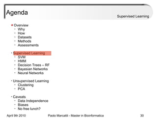
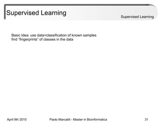
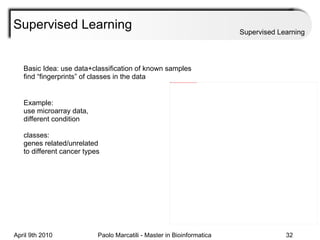
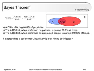
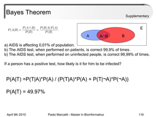
This document provides an overview of machine learning methods, including supervised and unsupervised learning. It discusses commonly used machine learning algorithms like support vector machines (SVM), hidden Markov models, decision trees, random forests, Bayesian networks, and neural networks. It also covers datasets, assessment metrics, and caveats to consider when using machine learning.

1. Machine Learning Methods: an overview Master in Bioinformatica – April 9th, 2010 Paolo Marcatili University of Rome “Sapienza” Dept. of Biochemical Sciences “Rossi Fanelli” [email_address] Overview Supervised Learning Unsupervised Learning Caveats

2. Agenda Overview Why How Datasets Methods Assessments Supervised Learning SVM HMM Decision Trees – RF Bayesian Networks Neural Networks Unsupervised Learning Clustering PCA Caveats Data Independence Biases No free lunch? Overview

3. Why Overview Large amount of data Large dimensionality

4. Large amount of data Large dimensionality Complex dynamics Data Noisiness Why Overview

5. Large amount of data Large dimensionality Complex dynamics Data Noisiness Computational efficiency Because we can Why Overview

6. How Numerical analysis Graphs Systems theory Geometry Statistics Probability!! Overview

7. How Numerical analysis Graphs Systems theory Geometry Statistics Probability!! Probability and statistics are fundamental They provide a solid framework for creating models and acquire knowledge Overview

8. Datasets Most common data used with ML: Genomes (genes, promoters, phylogeny, regulation...) Proteomes (secondary/tertiary structure, disorder, motifs, epitopes...) Clinical Data (drug evaluation, medical protocols, tool design...) Interactomic (PPI prediction and filtering, complexes...) Metabolomic (metabolic pathways identification, flux analysis, essentiality) Overview

9. Methods Machine Learning can Overview

10. Methods Machine Learning can Predict unknown function values Overview

11. Methods Machine Learning can Predict unknown function values Infer classes and assign samples Overview

12. Methods Machine Learning can Predict unknown function values Infer classes and assign samples Overview

13. Methods Machine Learning can not Overview

14. Methods Machine Learning can not Provide knowledge Overview

15. Methods Machine Learning can not Provide knowledge Overview

16. Methods Machine Learning can not Provide knowledge Learn Overview

17. Methods Information is In the data? In the model? Overview

18. Methods Work Schema: Choose a Learning-Validation Setting Prepare data (Training, Test, Validation sets) Train (1 or more times) Validate Use Overview

19. Love all, trust a few, do wrong to none. Overview 4 patients, 4 controls

20. Love all, trust a few, do wrong to none. Overview 2 more

21. Love all, trust a few, do wrong to none. Overview 10 more

22. Assessment Prediction of unknown data! Problems : Few data, robustness. Overview

23. Assessment Prediction of unknown data! Problems : Few data, robustness. Solutions : Training, Test and Validation sets Leave one Out K-fold Cross Validation Overview

24. Assessment 50% Training set : used to tune the model parameters 25% Test set : used to verify that the machine has “learnt” 25% Validation set : final assessment of the results Unfeasible with few data Overview

25. Assessment Leave-one-out: for each sample A i Training set : all the samples - { A i } Test set : { A i } Repeat Computationally intensive, good estimate of the mean error high variance Overview

26. Assessment K-fold cross validation: Divide your data in K subsets S 1..k Training set : all the samples - S i Test set : S i Repeat good compromise Overview

27. Assessment Sensitivity: TP/ [ TP + FN ] Given the disease is present, the likelihood of testing positive. Specificity: TN / [ TN + FP ] Given the disease is not present, the likelihood of testing negative. Positive Predictive Value : TP / [ TP + FP ] Given a test is positive, the likelihood disease is present Overview

28. Assessment Sensitivity: TP/ [ TP + FN ] Given the disease is present, the likelihood of testing positive. Specificity: TN / [ TN + FP ] Given the disease is not present, the likelihood of testing negative. Positive Predictive Value : TP / [ TP + FP ] Given a test is positive, the likelihood disease is present receiver operating characteristic (ROC) is a graphical plot of the sensitivity vs. (1 - specificity) for a binary classifier system as its discrimination threshold is varied. Overview

29. Assessment Overview Sensitivity: TP/ [ TP + FN ] Given the disease is present, the likelihood of testing positive. Specificity: TN / [ TN + FP ] Given the disease is not present, the likelihood of testing negative. Predictive Value Positive: TP / [ TP + FP ] Given a test is positive, the likelihood disease is present receiver operating characteristic (ROC) is a graphical plot of the sensitivity vs. (1 - specificity) for a binary classifier system as its discrimination threshold is varied. Area under ROC (AROC) is often used as a parameter to compare different classifiers

30. Agenda Supervised Learning Overview Why How Datasets Methods Assessments Supervised Learning SVM HMM Decision Trees – RF Bayesian Networks Neural Networks Unsupervised Learning Clustering PCA Caveats Data Independence Biases No free lunch?

31. Supervised Learning Supervised Learning Basic Idea: use data+classification of known samples find “fingerprints” of classes in the data

32. Supervised Learning Supervised Learning Basic Idea: use data+classification of known samples find “fingerprints” of classes in the data Example: use microarray data, different condition classes: genes related/unrelated to different cancer types

33. Supervised Learning Supervised Learning Basic Idea: use data+classification of known samples find “fingerprints” of classes in the data Example: use microarray data, different condition classes: genes related/unrelated to different cancer types

34. Support Vector Machines Supervised Learning Basic idea: Plot your data in an N-dimensional space Find the best hyperplane that separates the different classes Further samples can be classified using the region of the space they belong to

35. Support Vector Machines Supervised Learning length weight Fail Pass

36. Support Vector Machines Supervised Learning Fail Pass length weight Fail Pass margin

37. Support Vector Machines Supervised Learning Optimal Hyperplane (OHP) simple kind of SVM (called an LSVM ) maximum margin Fail Pass length weight Fail Pass margin Support vectors

38. Support Vector Machines Supervised Learning What if data are not linearly separable? Original Data

39. Support Vector Machines Supervised Learning What if data are not linearly separable? Allow mismatches soft margins (add a weight matrix) Original Data Original Data

40. Support Vector Machines Supervised Learning Hyperplane What if data are not linearly separable? weight 2 length 2 weight * length Original Data

41. Support Vector Machines Supervised Learning Only Inner product is needed to calculate Dual problem and decision function Hypersurface Kernelization Hyperplane What if data are not linearly separable? The Kernel trick! weight 2 length 2 weight * length length Original Data

42. SVM example Supervised Learning Knowledge-based analysis of microarray gene expression data by using support vector machines Michael P. S. Brown*, William Noble Grundy †‡ , David Lin*, Nello Cristianini § , Charles Walsh Sugnet ¶ , Terrence S. Furey*, Manuel Ares, Jr. ¶ , and David Haussler* We introduce a method of functionally classifying genes by using gene expression data from DNA microarray hybridization experiments. The method is based on the theory of support vector machines (SVMs). SVMs are considered a supervised computer learning method because they exploit prior knowledge of gene function to identify unknown genes of similar function from expression data. SVMs avoid several problems associated with unsupervised clustering methods, such as hierarchical clustering and self-organizing maps. SVMs have many mathematical features that make them attractive for gene expression analysis, including their flexibility in choosing a similarity function, sparseness of solution when dealing with large data sets, the ability to handle large feature spaces, and the ability to identify outliers. We test several SVMs that use different similarity metrics, as well as some other supervised learning methods, and find that the SVMs best identify sets of genes with a common function using expression data. Finally, we use SVMs to predict functional roles for uncharacterized yeast ORFs based on their expression data. To judge overall performance, we define the cost of using the method M as C ( M ) 5 fp ( M ) 1 2 z fn ( M ), where fp ( M ) is the number of false positives for method M , and fn ( M ) is the number of false negatives for method M . The false negatives are weighted more heavily than the false positives because, for these data, the number of positive examples is small compared with the number of negatives.

43. Hidden Markov Models Supervised Learning There is a regular and a biased coin. You don't know which one is being used. During the game the coins are exchanged with a certain fixed probability All you know is the output sequence

44. Hidden Markov Models Supervised Learning There is a regular and a biased coin. You don't know which one is being used. During the game the coins are exchanged with a certain fixed probability All you know is the output sequence HHTHTHTHTHTTTTHTHHTHHHHHHHHHTHTHTHHTHTHHHHTHTH Given a set the parameters, which is the probability of the output seq.? Which parameters are more likely to have produced the output? Which coin was being used at a certain point of the sequence?

45. Hidden Markov Models Supervised Learning

46. Decision trees Supervised Learning Mimics the behavior of an expert

47. Decision trees Supervised Learning Mimics the behavior of an expert

48. Mimics the behavior of an expert Decision trees Supervised Learning

49. Mimics the behavior of an expert Decision trees Supervised Learning

50. Pros: Easy to interpreter Statistical analysis Informative results Cons: A single variable Not optimal Not robust Majority rules! Decision trees Supervised Learning

51. Random Forests Supervised Learning Split the data in several subsets, construct a DT for each set Each DT expresses a vote, the majority wins Much more accurate and robust (bootstrap)

52. Random Forests Supervised Learning Split the data in several subsets, construct a DT for each set Each DT expresses a vote, the majority wins Much more accurate and robust (bootstrap) Prediction of protein–protein interactions using random decision forest framework Xue-Wen Chen * and Mei Liu Motivation: Protein interactions are of biological interest because they orchestrate a number of cellular processes such as metabolic pathways and immunological recognition. Domains are the building blocks of proteins; therefore, proteins are assumed to interact as a result of their interacting domains. Many domain-based models for protein interaction prediction have been developed, and preliminary results have demonstrated their feasibility. Most of the existing domain-based methods, however, consider only single-domain pairs (one domain from one protein) and assume independence between domain–domain interactions. Results: In this paper, we introduce a domain-based random forest of decision trees to infer protein interactions. Our proposed method is capable of exploring all possible domain interactions and making predictions based on all the protein domains. Experimental results on Saccharomyces cerevisiae dataset demonstrate that our approach can predict protein–protein interactions with higher sensitivity (79.78%) and specificity (64.38%) compared with that of the maximum likelihood approach. Furthermore, our model can be used to infer interactions not only for single-domain pairs but also for multiple domain pairs.

53. Bayesian Networks Supervised Learning The probabilistic approach is extremely powerful but requires a huge amount of information/data for a complete representation Not all correlations or cause-effect relationships between variables are significative

54. Bayesian Networks Supervised Learning The probabilistic approach is extremely powerful but requires a huge amount of information/data for a complete representation Not all correlations or cause-effect relationships between variables are significative Consider only meaningful links!

55. Bayesian Networks Supervised Learning I'm at work, neighbor John calls to say my alarm is ringing, but neighbor Mary doesn't call. Sometimes it's set off by minor earthquakes. Is there a burglar? Variables: Burglary , Earthquake , Alarm , JohnCalls , MaryCalls Network topology reflects "causal" knowledge: A burglar can set the alarm off An earthquake can set the alarm off The alarm can cause Mary to call The alarm can cause John to call

56. Bayesian Networks Supervised Learning I'm at work, neighbor John calls to say my alarm is ringing, but neighbor Mary doesn't call. Sometimes it's set off by minor earthquakes. Is there a burglar? Variables: Burglary , Earthquake , Alarm , JohnCalls , MaryCalls Network topology reflects "causal" knowledge: A burglar can set the alarm off An earthquake can set the alarm off The alarm can cause Mary to call The alarm can cause John to call Bayes Theorem again!

57. Bayesian Networks Supervised Learning We don't know the joint probability distribution, how can we learn it from the data? Optimize the likelyhood , i.e. the probability that the model generated the data Maximum likelyhood (simplest) Maximum posterior Marginal likelyhood (hardest) We don't know which relationship is present between variables, how can we learn it from the data? Connections in a graph are over-exponential, enumeration is impossible Euristics, random sampling, monte carlo Does independence assumption hold? Is the correlation informative? (BIC, Occam's razor, AIC)

58. Neural Networks Supervised Learning Neural Networks interpolate functions They have nothing to do with brains

59. Neural Networks Supervised Learning Neural Networks interpolate functions They have nothing to do with brains

60. Neural Networks Supervised Learning Neural Networks interpolate functions They have nothing to do with brains

61. Neural Networks Supervised Learning Parameter settings:

62. Neural Networks Supervised Learning Parameter settings: avoid overfitting

63. Neural Networks Supervised Learning Parameter settings: avoid overfitting Learning --> validation --> usage No underlying model, but it often works

64. Neural Networks Supervised Learning Protein Disorder Prediction: Implications for Structural Proteomics Rune Linding, 1,4, * Lars Juhl Jensen, 1,2,4 Francesca Diella, 3 Peer Bork, 1,2 Toby J. Gibson, 1 and Robert B. Russell 1 Abstract A great challenge in the proteomics and structural genomics era is to predict protein structure and function, including identification of those proteins that are partially or wholly unstructured. Disordered regions in proteins often contain short linear peptide motifs (e.g., SH3 ligands and targeting signals) that are important for protein function. We present here DisEMBL, a computational tool for prediction of disordered/unstructured regions within a protein sequence. As no clear definition of disorder exists, we have developed parameters based on several alternative definitions and introduced a new one based on the concept of “hot loops,” i.e., coils with high temperature factors. Avoiding potentially disordered segments in protein expression constructs can increase expression, foldability, and stability of the expressed protein. DisEMBL is thus useful for target selection and the design of constructs as needed for many biochemical studies, particularly structural biology and structural genomics projects. The tool is freely available via a web interface (http://dis.embl.de) and can be downloaded for use in large-scale studies.

65. Agenda Unsupervised Learning Overview Why How Datasets Methods Assessments Supervised Learning SVM HMM Decision Trees – RF Bayesian Networks Neural Networks Unsupervised Learning Clustering PCA Caveats Data Independence Biases No free lunch?

66. Unsupervised Learning Unsupervised Learning If we have no idea of actual data classification, we can try to guess

67. Clustering Unsupervised Learning Put together similar objects to define classes

68. Clustering Unsupervised Learning Put together similar objects to define classes

69. Clustering Unsupervised Learning K-means Hierarchical top-down Hierarchical down-up Fuzzy Put together similar objects to define classes How?

70. Clustering Unsupervised Learning Euclidean Correlation Spearman Rank Manhattan Put together similar objects to define classes Which metric? How?

71. Clustering Unsupervised Learning Put together similar objects to define classes Which metric? Which “shape”? Compact Concave Outliers Inner radius cluster separation How?

72. Hierarchical Clustering Unsupervised Learning We start with every data point in a separate cluster We keep merging the most similar pairs of data points/clusters until we have one big cluster left This is called a bottom-up or agglomerative method

73. Hierarchical Clustering Unsupervised Learning We start with every data point in a separate cluster We keep merging the most similar pairs of data points/clusters until we have one big cluster left This is called a bottom-up or agglomerative method

74. Hierarchical Clustering Unsupervised Learning We start with every data point in a separate cluster We keep merging the most similar pairs of data points/clusters until we have one big cluster left This is called a bottom-up or agglomerative method

75. Hierarchical Clustering Unsupervised Learning We start with every data point in a separate cluster We keep merging the most similar pairs of data points/clusters until we have one big cluster left This is called a bottom-up or agglomerative method

76. Hierarchical Clustering Unsupervised Learning We start with every data point in a separate cluster We keep merging the most similar pairs of data points/clusters until we have one big cluster left This is called a bottom-up or agglomerative method

77. Hierarchical Clustering Unsupervised Learning We start with every data point in a separate cluster We keep merging the most similar pairs of data points/clusters until we have one big cluster left This is called a bottom-up or agglomerative method

78. Hierarchical Clustering Unsupervised Learning We start with every data point in a separate cluster We keep merging the most similar pairs of data points/clusters until we have one big cluster left This is called a bottom-up or agglomerative method

79. Hierarchical Clustering Unsupervised Learning We start with every data point in a separate cluster We keep merging the most similar pairs of data points/clusters until we have one big cluster left This is called a bottom-up or agglomerative method 

80. K-means Unsupervised Learning Start with K random centers Assign each sample to the closest center Recompute centers (samples average) Repeat until converged

81. K-means Unsupervised Learning Start with K random centers Assign each sample to the closest center Recompute centers (samples average) Repeat until converged

82. K-means Unsupervised Learning Start with K random centers Assign each sample to the closest center Recompute centers (samples average) Repeat until converged

83. K-means Unsupervised Learning Start with K random centers Assign each sample to the closest center Recompute centers (samples average) Repeat until converged

84. K-means Unsupervised Learning Start with K random centers Assign each sample to the closest center Recompute centers (samples average) Repeat until converged

85. K-means Unsupervised Learning Start with K random centers Assign each sample to the closest center Recompute centers (samples average) Repeat until converged

86. K-means Unsupervised Learning Start with K random centers Assign each sample to the closest center Recompute centers (samples average) Repeat until converged

87. K-means Unsupervised Learning Start with K random centers Assign each sample to the closest center Recompute centers (samples average) Repeat until converged

88. K-means Unsupervised Learning Start with K random centers Assign each sample to the closest center Recompute centers (samples average) Repeat until converged

89. K-means Unsupervised Learning Start with K random centers Assign each sample to the closest center Recompute centers (samples average) Repeat until converged

90. K-means Unsupervised Learning Start with K random centers Assign each sample to the closest center Recompute centers (samples average) Repeat until converged

91. K-means Unsupervised Learning Start with K random centers Assign each sample to the closest center Recompute centers (samples average) Repeat until converged

92. K-means Unsupervised Learning Start with K random centers Assign each sample to the closest center Recompute centers (samples average) Repeat until converged

93. K-means Unsupervised Learning Start with K random centers Assign each sample to the closest center Recompute centers (samples average) Repeat until converged

94. K-means Unsupervised Learning Start with K random centers Assign each sample to the closest center Recompute centers (samples average) Repeat until converged

95. K-means Unsupervised Learning Start with K random centers Assign each sample to the closest center Recompute centers (samples average) Repeat until converged

96. K-means Unsupervised Learning Start with K random centers Assign each sample to the closest center Recompute centers (samples average) Repeat until converged

97. K-means Unsupervised Learning Start with K random centers Assign each sample to the closest center Recompute centers (samples average) Repeat until converged

98. K-means Unsupervised Learning Start with K random centers Assign each sample to the closest center Recompute centers (samples average) Repeat until converged

99. K-means Unsupervised Learning Start with K random centers Assign each sample to the closest center Recompute centers (samples average) Repeat until converged

100. K-means Unsupervised Learning Start with K random centers Assign each sample to the closest center Recompute centers (samples average) Repeat until converged

101. K-means Unsupervised Learning Start with K random centers Assign each sample to the closest center Recompute centers (samples average) Repeat until converged

102. K-means Unsupervised Learning Start with K random centers Assign each sample to the closest center Recompute centers (samples average) Repeat until converged

103. K-means Unsupervised Learning Start with K random centers Assign each sample to the closest center Recompute centers (samples average) Repeat until converged

104. K-means Unsupervised Learning Start with K random centers Assign each sample to the closest center Recompute centers (samples average) Repeat until converged

105. K-means Unsupervised Learning Start with K random centers Assign each sample to the closest center Recompute centers (samples average) Repeat until converged

106. K-means Unsupervised Learning Start with K random centers Assign each sample to the closest center Recompute centers (samples average) Repeat until converged

107. K-means Unsupervised Learning Start with K random centers Assign each sample to the closest center Recompute centers (samples average) Repeat until converged

108. PCA Unsupervised Learning Multidimensional data (hard to visualize) Data variability is not equally distributed

109. PCA Unsupervised Learning Multidimensional data (hard to visualize) Data variability is not equally distributed Correlation between variables Change coordinate system, remove correlation retain only most variable coordinates How: (generalized eigenvectors, SVD) Pro: noise (and information) reduction

110. Agenda Caveats Overview Why How Datasets Methods Assessments Supervised Learning SVM HMM Decision Trees – RF Bayesian Networks Neural Networks Unsupervised Learning Clustering PCA Caveats Data Independence Biases No free lunch?

111. Data independence Training set, Test set and Validation set must be clearly separated E.g. neural network to infer gene function from sequence training set: annotated gene sequences, deposit date before Jan 2007 test set: annotated gene sequences, deposit date after Jan 2007 But annotation of new sequences is often inferred from old sequences! Caveats

112. Biases Data should be unbiased, i.e. it should be a good sample of our “space” E.g. neural network to find disordered regions training set: solved structures, residues in SEQRES but not in ATOM But solved structures are typically small, globular, cytoplasmatic proteins Caveats

113. Take-home message Always look at data. ML methods are extremely error-prone Use probability and statistics were possible In this order: Model, Data, Validation, Algorithm Be careful with biases, redundancy, hidden variables Occam's Razor: simpler is better Be careful with overfitting and overparametrizing Common sense is a powerful tool (but don't abuse it) Caveats

114. References Needham CJ, Bradford JR, Bulpitt AJ, Westhead DR (2007) A Primer on Learning in Bayesian Networks for Computational Biology. PLoS Comput Biol 3(8): e129. doi:10.1371/journal.pcbi.0030129 Tarca AL, Carey VJ, Chen X-w, Romero R, Dr ă ghici S (2007) Machine Learning and Its Applications to Biology. PLoS Comput Biol 3(6): e116. doi:10.1371/journal.pcbi.0030116 Sean R Eddy (2004) What is a hidden Markov model? Nature Biotechnology 22, 1315 - 1316 (2004) doi:10.1038/nbt1004-1315 http ://see.stanford.edu/see/courseinfo.aspx?coll=348ca38a-3a6d-4052-937d-cb017338d7b1

115. Bayes Theorem Supplementary a) AIDS is affecting 0,01% of population. b) The AIDS test, when performed on patients, is correct 99,9% of times. b) The AIDS test, when performed on uninfected people, is correct 99,99% of times. If a person has a positive test, how likely is it for him to be infected? A B A  B E

116. Bayes Theorem Supplementary a) AIDS is affecting 0,01% of population. b) The AIDS test, when performed on patients, is correct 99,9% of times. b) The AIDS test, when performed on uninfected people, is correct 99,99% of times. If a person has a positive test, how likely is it for him to be infected? P(A|T) =P(T|A)*P(A) / (P(T|A)*P(A) + P(T|¬A)*P(¬A)) P(A|T) = 49.97% A B A  B E