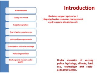
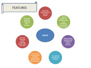
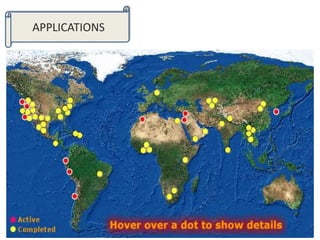
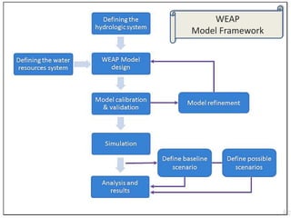
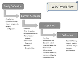
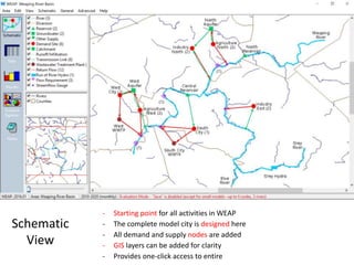
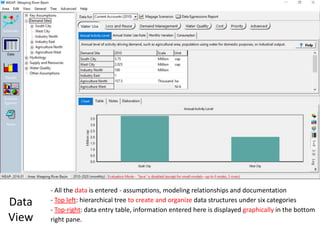
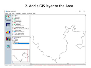
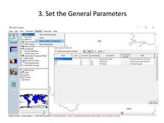
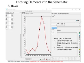
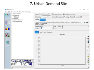
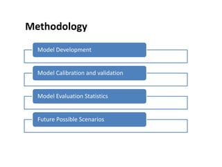
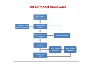
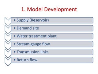
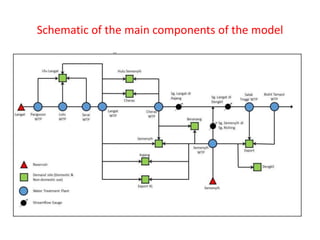
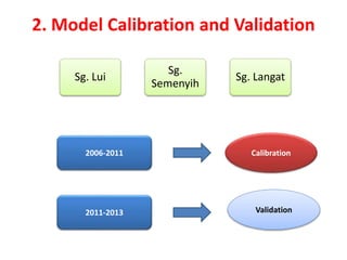
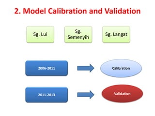
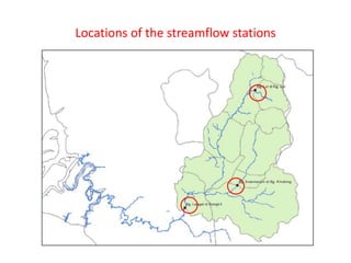
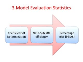
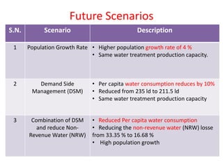
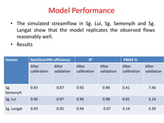
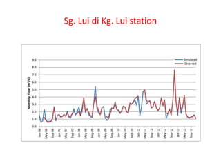
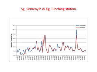
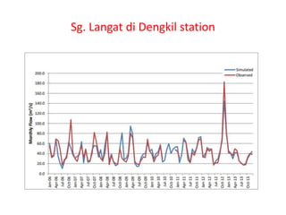
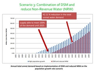
The document describes WEAP (Water Evaluation and Planning), a water resources planning model. It provides an overview of WEAP's features and capabilities for integrated water resources management. These include built-in models, a model-building interface, reporting tools, and a GIS-based graphical user interface. The document then presents a case study application of WEAP for the Langat River Basin in Malaysia to investigate water supply and demand trends and assess water availability under future scenarios. The WEAP model developed for the basin was calibrated and validated and able to reasonably simulate streamflows. Modeling results show increasing future water deficits without intervention and the benefits of demand management and reduction of non-revenue water losses.

1. WEAP
Water Evaluation And Planning
By:
Iqura Malik
(17WM60R02)
School of Water Resources
IIT Kharagpur
Sapna Gautam
(17WM60R08)
Navdesh Nirwan
(17WM60R09)

2. IntroductionWater demand
Supply and runoff
Evapotranspiration
Crop irrigation requirements
Instream flow requirements
Groundwater and surface storage
Pollution generation
Discharge and instream water
quality
Under scenarios of varying
policy, hydrology, climate, land
use, technology and socio-
economic factors.
Decision support system for I
ntegrated water resources management
used to create simulations of:

3. Integrated
water resources
planning
system
Built-in
models for:
Rainfall runoff
and
infiltration,
evapotranspirat
ion, crop,etc.
Model-building
capability with
a number of
built-in
functions
User-defined
variables and
equations
Dynamic links
to spreadsheets
and other
models Flexible
and expandable
data structures
Powerful
reporting
system
including
graphs, tables
and maps
GIS-based,
graphical
"drag and
drop"
interface
WEAP
FEATURES

4. APPLICATIONS

5. WEAP
Model Framework

6. Study Definition
Current Accounts
Scenarios
Evaluation
- Time horizon
- Spatial boundaries
- System components
- Network
Configuration - Demand
- River Simulation
- Pollutant Generation
- Resources and
Supplies
- Wastewater
Treatment
- Reservoir
Characteristics
- Hydrology
- Demographic and
Economic activity
- Patterns of water use
- Water system
infrastructure
- Allocation and Pricing
- Environmental policy
- Component costs
- Water Sufficiency
- Pollutant loadings
- Sensitivity analysis
- Ecosystem
Requirements
WEAP Work Flow

7. BASIC STRUCTURE OF THE
MODEL

8. Schematic
View
- Starting point for all activities in WEAP
- The complete model city is designed here
- All demand and supply nodes are added
- GIS layers can be added for clarity
- Provides one-click access to entire

9. Data
View
- All the data is entered - assumptions, modeling relationships and documentation
- Top left: hierarchical tree to create and organize data structures under six categories
- Top-right: data entry table, information entered here is displayed graphically in the bottom
right pane.

10. Results View
- Displays charts and tables covering each aspect of the
system: demand, supply, costs, and environmental loadings
- Customizable reports for one or more scenarios

11. Scenario
Explorer View
- Scenarios are compared here
- help demonstrate the impact of various assumptions and policies on results
- input values can be changed and WEAP will recalculate and update the results.

12. Notes View
- tool for entering documentation and self-study references

13. Input data Requirement
• Schematic maps of the area
• Supply and Demand data
• Transmission link data
• Hydrology
• Groundwater
• Reservoirs
• Surface Water Quality and
Wastewater Treatment
Facilities.
• Other Supply Sources
(imports, transfers,
desalinization, etc.)
 Satellite image
 Municipality
 State Drainage and
Irrigation Deptt.

14. HOWTO
RUNTHE MODEL?

16. 1. Create a New Area

18. Set study area Boundaries

19. 2. Add a GIS layer to the Area

20. 3. Set the General Parameters

21. Entering Elements into the Schematic
6. River
 Draw the River
- Double-click on River in schematic view
- Take cursor to the head and start
drawing
- Name the river
Enter Data in the River
- Go to Data View tab
- Select Supply and Resources >
River
- Monthly Time-Series Wizard
- Enter headflow data

22. • Pull demand node and
release
• Name the site and set
Demand Priority
7. Urban Demand Site

23. 8. Agricultural Demand Site &
Other Supply Sites

24. 9. Create Transmission Links

25. 10. Create Return Flow Links

26. Creating Scenarios
• A “Reference” scenario is established from the Current
Accounts to simulate evolution of the system without
intervention.
• Finally, “what-if” scenarios can be created to alter the
“Reference Scenario” and evaluate the effects of
changes in policies and/or technologies.

27. Add Key Assumptions

28. Define Units

29. Enter Monthly Variation

30. Enter Values

31. Create Reference Scenario

42. Run the Reference Scenario

46. Create a New Scenario to Model High
Population Growth

49. Enter the Data for this Scenario

55. Case Study
Application of
Water Evaluation and Planning Model
for Integrated Water Resources Management
in Langat River Basin, Malaysia

56. Objective of the study
• To investigate the trend of supply and demand in Langat
catchment.
• To assess the water availability with population growth in
Langat Catchment using Water Evaluation and Planning
(WEAP).

57. Study Area: The Langat River
• Located in south-eastern parts of the
Selangor state of Malaysia.
• Study focused on the upper Langat River
basin
• Basin area - 2350 km2
• River length - 182 km
• Average annual rainfall - 2145 mm
• Annual evapotranspiration - 1500 mm
• There two 2 reservoirs and 8 water
treatment plants within the basin.
• Major tributaries of the basin: Langat
River, Semenyih River and Labu River.

58. Data
Requirement

59. Methodology
Model Development
Model Calibration and validation
Model Evaluation Statistics
Future Possible Scenarios

60. WEAP model framework

61. 1. Model Development
• Supply (Reservoir)
• Demand site
• Water treatment plant
• Stream-gauge flow
• Transmission links
• Return flow

62. Schematic of the main components of the model

63. 2. Model Calibration and Validation
2006-2011 Calibration
2011-2013 Validation
Sg. Lui
Sg.
Semenyih
Sg. Langat

64. 2. Model Calibration and Validation
2006-2011 Calibration
2011-2013 Validation
Sg. Lui
Sg.
Semenyih
Sg. Langat

65. Locations of the streamflow stations

66. 3.Model Evaluation Statistics

67. Coefficient of determination (R2 )
• Outlines the degree of collinearity between simulated and
measured data

68. Nash-Sutcliffe efficiency
• NSE indicates how well the plot of observed versus simulated
data fits the 1:1 line.
• NSE ranges between −∞ and 1.0
• Values between 0.0 and 1.0 are acceptable.

69. Percent bias (PBIAS)
• Measures the average tendency of the simulated data to be
larger or smaller than their observed ones.
• The optimal value of PBIAS is 0.
• Positive values indicate model underestimation bias
• Negative values indicate model overestimation bias
Where,
Yi obs : the ith observed streamflow
Yi sim: the ith simulated streamflow

70. Future possible Scenarios
• Current water- use
• Population growth at 2.57%.
REFERENCE
SCENARIO
POPULATION
GROWTH DEMAND
MANAGEMENT
SIDE
SUPPLY SIDE
MANAGEMENT

71. Future Scenarios
S.N. Scenario Description
1 Population Growth Rate • Higher population growth rate of 4 %
• Same water treatment production capacity.
2 Demand Side
Management (DSM)
• Per capita water consumption reduces by 10%
• Reduced from 235 ld to 211.5 ld
• Same water treatment production capacity
3 Combination of DSM
and reduce Non-
Revenue Water (NRW)
• Reduced Per capita water consumption
• Reducing the non-revenue water (NRW) losse
from 33.35 % to 16.68 %
• High population growth

72. RESULTS

73. Model Performance
• The simulated streamflow in Sg. Lui, Sg. Semenyih and Sg.
Langat show that the model replicates the observed flows
reasonably well.
• Results
Stream NashSutcliffe efficiency R2 PBIAS %
After
calibration
After
validation
After
calibration
After
validation
After
calibration
After
validation
Sg.
Semenyih
0.93 0.87 0.93 0.98 0.41 7.96
Sg. Lui 0.96 0.97 0.96 0.98 0.81 3.14
Sg. Langat 0.93 0.92 0.94 0.97 4.14 4.39

74. Sg. Lui di Kg. Lui station

75. Sg. Semenyih di Kg. Rinching station

76. Sg. Langat di Dengkil station

77. Reference scenario
• Water demand would steadily rise by 2.57 % annually from
2005 to 2050.
• Projected water demand rises to a maximum of 599.43 MCM
from 300 MCM
• Langat basin area will face water deficits for both domestic
and non-domestic sectors by the year of 2019.
• 38 % of the treated water were supplied for areas outside of
Langat basin.

78. Annual total water demand and unmet demand
of reference and population growth scenarios
Scenario 1: Population Growth Rate
Unmet demand rises by twice
than in reference scenario.water deficits in 2017

79. Annual total unmet demand based on implementation of DSM on the reference scenario
Scenario 2: Demand Side Management (DSM)
42.11 % reduction in the total unmet water demand

80. Annual total unmet demand based on implementation of DSM and reduced NRW on the
population growth rate scenario
Scenario 3: Combination of DSM and
reduce Non-RevenueWater (NRW)
supply able to meet 100%
of the demand until 2025
42.11 % reduction in the total
unmet water demand

81. Conclusion
• The model developed through WEAP is highly capable and
showed great performance to manage available water
resources with water demand.
• Model outputs scientifically sound, robust and defensible
• Model able to simulate various possible future scenarios.
• Capable to resolve conflicts over water allocation.
• Should consider Non point sources.

82. Future scope of the study
• WEAP model assumes an unlimited groundwater supply.
• Model should be expanded to include realistic estimates of
aquifer performance, including recharge.
• Following the scenario system already used in the Water
Plan, you might begin by developing at least three alternatives
for the annual net loss to the aquifer and apply these both to
current conditions and to the future scenarios being
examined.
• It should also consider non-point sources.