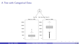
Download as PDF, PPTX
![Rules
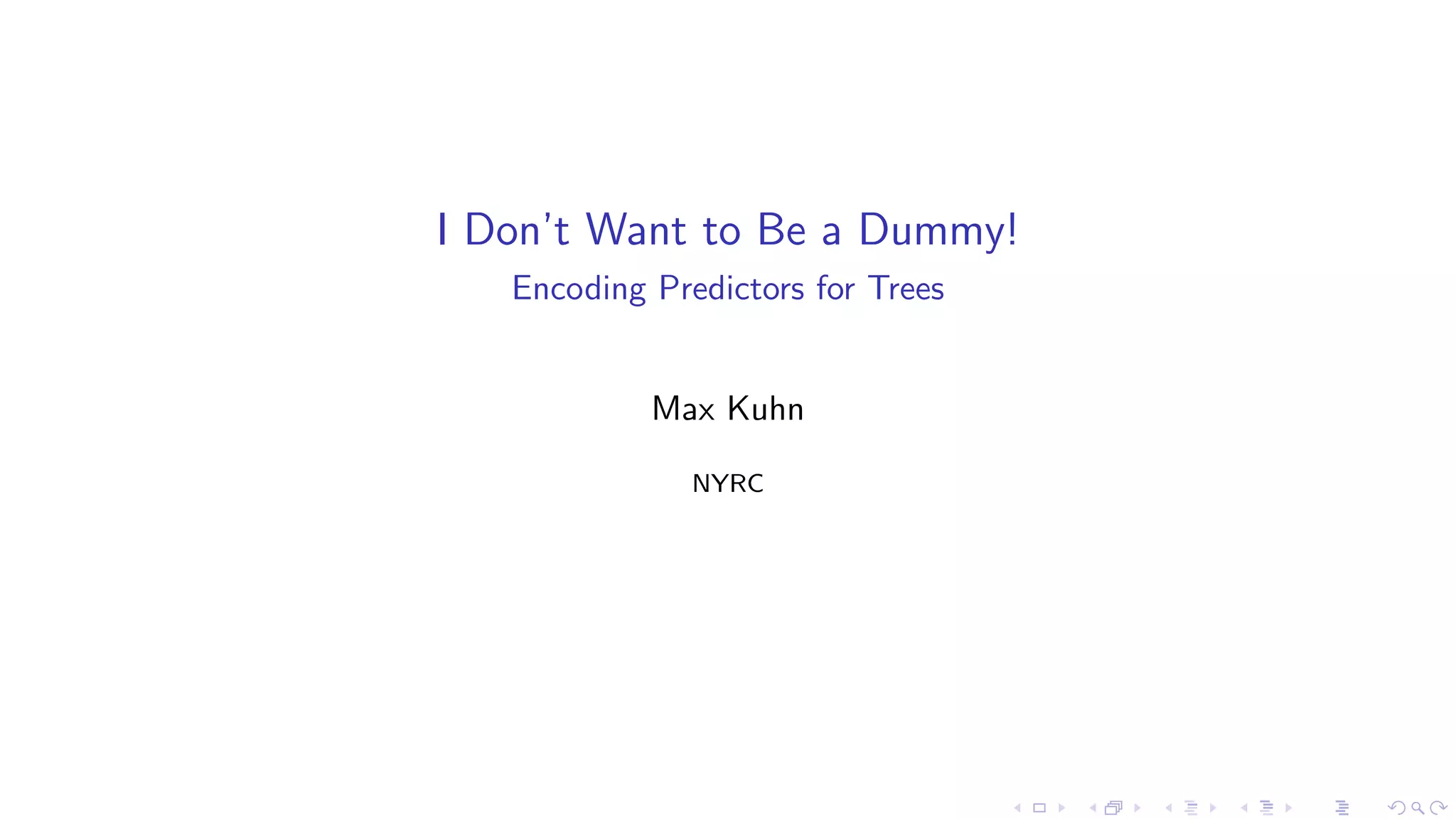
Similarly, rule–based models are non–nested sets of if statements:
> library(C50)
> summary(C5.0(Class ~ ., data = schedulingData, rules = TRUE))
<snip>
Rule 109: (17/7, lift 9.7)
Protocol in {F, J, N}
Compounds > 818
InputFields > 152
NumPending <= 0
Hour > 0.6333333
Day = Tue
-> class L [0.579]
Default class: VF
Max Kuhn (NYRC) I Don’t Want to Be a Dummy! 3 / 16](https://image.slidesharecdn.com/friday1pmmaxkuhn-160511203810/85/I-Don-t-Want-to-Be-a-Dummy-Encoding-Predictors-for-Trees-3-320.jpg)
![Bayes!
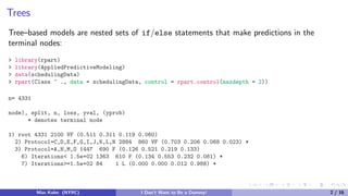
Bayesian regression and classification models don’t really specify anything about the predictors
beyond Pr[X] and Pr[X|Y ].
If there were only one categorical predictor, we could have Pr[X|Y ] be a table of raw
probabilities:
> xtab <- table(schedulingData$Day, schedulingData$Class)
> apply(xtab, 2, function(x) x/sum(x))
VF F M L
Mon 0.1678 0.1492 0.15 0.162
Tue 0.1913 0.2019 0.27 0.255
Wed 0.2090 0.2101 0.19 0.228
Thu 0.1678 0.1589 0.18 0.154
Fri 0.2171 0.2183 0.20 0.178
Sat 0.0068 0.0082 0.00 0.023
Sun 0.0403 0.0535 0.00 0.000
Max Kuhn (NYRC) I Don’t Want to Be a Dummy! 4 / 16](https://image.slidesharecdn.com/friday1pmmaxkuhn-160511203810/85/I-Don-t-Want-to-Be-a-Dummy-Encoding-Predictors-for-Trees-4-320.jpg)
![Dummy Variables
For the other models, we typically encode a predictor with C categories into C − 1 binary
dummy variables:
> design_mat <- model.matrix(Class ~ Day, data = head(schedulingData))
> design_mat[, colnames(design_mat) != "(Intercept)"]
DayTue DayWed DayThu DayFri DaySat DaySun
1 1 0 0 0 0 0
2 1 0 0 0 0 0
3 0 0 1 0 0 0
4 0 0 0 1 0 0
5 0 0 0 1 0 0
6 0 1 0 0 0 0
In this case, one predictor generates six columns in the design matrix
Max Kuhn (NYRC) I Don’t Want to Be a Dummy! 5 / 16](https://image.slidesharecdn.com/friday1pmmaxkuhn-160511203810/85/I-Don-t-Want-to-Be-a-Dummy-Encoding-Predictors-for-Trees-5-320.jpg)
![R and Dummy Variables
In almost all cases, using a formula with a model function will convert factors to dummy
variables.
However, some do not (e.g. rpart, randomForest, gbm, C5.0, NaiveBayes, etc.). This
makes sense for these models.
If you are tuning your model with train, the formula method will create dummy variables and
the non–formula method does not:
> ## dummy variables presented to underlying model:
> train(Class ~ ., data = schedulingData, ...)
>
> ## any factors are preserved
> train(x = schedulingData[, -ncol(schedulingData)],
+ y = schedulingData$Class,
+ ...)
Max Kuhn (NYRC) I Don’t Want to Be a Dummy! 16 / 16](https://image.slidesharecdn.com/friday1pmmaxkuhn-160511203810/85/I-Don-t-Want-to-Be-a-Dummy-Encoding-Predictors-for-Trees-16-320.jpg)

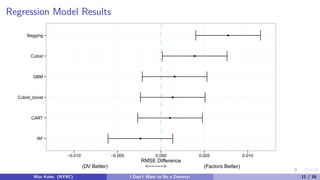
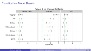
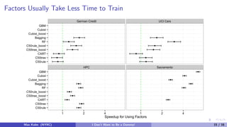
The document discusses tree-based models and the importance of encoding categorical predictors as dummy variables or factors in predictive modeling. It presents various modeling techniques and evaluates their performance on different datasets, highlighting that the choice of encoding can significantly affect model accuracy and training speed. Additionally, it concludes that the encoding decision should consider the nature of the data and the specific modeling approach used.


![Hacking-Uncovered-How-People-Get-Hacked-and-How-to-Stay-Safe[1].pptx](https://cdn.slidesharecdn.com/ss_thumbnails/hacking-uncovered-how-people-get-hacked-and-how-to-stay-safe1-260130170011-4883a9c7-thumbnail.jpg?width=640&height=640&fit=bounds)


