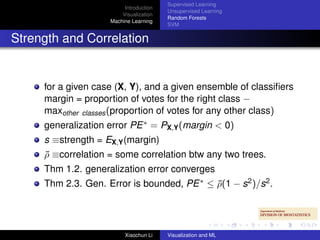
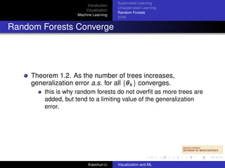
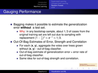
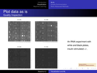
Introduction
             Visualization
         Machine Learning


Visualization and Machine Learning
      for exploratory data analysis


                Xiaochun Li1,2
              1 Division of Biostatistics

       Indiana University School of Medicine
               2 Regenstrief   Institute


    May 2, 2008 / CCBB Journal Club


              Xiaochun Li      Visualization and ML
Introduction
                         Visualization
                     Machine Learning


Outline

  1   Introduction

  2   Visualization
         As Is
         Simple Summarization
         More Advanced Methods

  3   Machine Learning
        Supervised Learning
        Unsupervised Learning
        Random Forests
        SVM


                          Xiaochun Li    Visualization and ML
Introduction
                          Visualization
                      Machine Learning


Introduction


  Mining large scale datasets, methods are needed to
      search for patterns, e.g., biologically important gene sets,
      or samples
      present data structure succinctly
      both are essential in the analysis.


                           Xiaochun Li    Visualization and ML
Introduction   As Is
                               Visualization   Simple Summarization
                           Machine Learning    More Advanced Methods


Objective
Visualization


    An essential part of exploratory data analysis, and reporting the
    results.
         plot data as is
         plot data after simple summarization
         plot data based on more advanced methods
                clustering
                PCA (Principal component analysis)
                MDS (Multidimensional scaling)
                Silhouette, randomForest, . . .


                                Xiaochun Li    Visualization and ML
Introduction   As Is
                         Visualization   Simple Summarization
                     Machine Learning    More Advanced Methods


Outline

  1   Introduction

  2   Visualization
         As Is
         Simple Summarization
         More Advanced Methods

  3   Machine Learning
        Supervised Learning
        Unsupervised Learning
        Random Forests
        SVM


                          Xiaochun Li    Visualization and ML
Introduction   As Is
                         Visualization   Simple Summarization
                     Machine Learning    More Advanced Methods


Plot data as is
Quality Inspection


                                                                An affymetrics chip
                                                                image. Some images
                                                                may have obvious local
                                                                contaminations.


                          Xiaochun Li    Visualization and ML
Introduction           As Is
                                    Visualization           Simple Summarization
                                Machine Learning            More Advanced Methods


Plot data as is
Quality Inspection
             Ins+, white                      Ins−, white

                           1                                         1

                           2                                         2

                           3                                         3

                           4                                         4

                           5                                         5

                           6                                         6

                           7                                         7

                           8                                         8

                           9                                         9

                           10                                        10

                           11                                        11

                           12                                        12

                           13                                        13

                           14                                        14

                           15                                        15

                           16                                        16

                                                                                   An RNAi experiment with
     1
     2
     3
     4
     5
     6
     7
     8
     9
    10
    11
    12
    13
    14
    15
    16
    17
    18
    19
    20
    21
    22
    23
    24


                                   1
                                   2
                                   3
                                   4
                                   5
                                   6
                                   7
                                   8
                                   9
                                  10
                                  11
                                  12
                                  13
                                  14
                                  15
                                  16
                                  17
                                  18
                                  19
                                  20
                                  21
                                  22
                                  23
                                  24
             Ins+, black                      Ins−, black
                                                                                   white and black plates,
                           1

                           2
                                                                     1

                                                                     2
                                                                                   insulin stimulated +/-.
                           3                                         3

                           4                                         4

                           5                                         5

                           6                                         6

                           7                                         7

                           8                                         8

                           9                                         9

                           10                                        10

                           11                                        11

                           12                                        12

                           13                                        13

                           14                                        14

                           15                                        15

                           16                                        16
     1
     2
     3
     4
     5
     6
     7
     8
     9
    10
    11
    12
    13
    14
    15
    16
    17
    18
    19
    20
    21
    22
    23
    24


                                   1
                                   2
                                   3
                                   4
                                   5
                                   6
                                   7
                                   8
                                   9
                                  10
                                  11
                                  12
                                  13
                                  14
                                  15
                                  16
                                  17
                                  18
                                  19
                                  20
                                  21
                                  22
                                  23
                                  24


                                     Xiaochun Li            Visualization and ML
Introduction   As Is
                            Visualization   Simple Summarization
                        Machine Learning    More Advanced Methods


Plot data as is
R tools


          image or heatmap for any chip arrays
          for cell-based assays, could also use plotPlate in R
          package prada


                             Xiaochun Li    Visualization and ML
Introduction   As Is
                         Visualization   Simple Summarization
                     Machine Learning    More Advanced Methods


Outline

  1   Introduction

  2   Visualization
         As Is
         Simple Summarization
         More Advanced Methods

  3   Machine Learning
        Supervised Learning
        Unsupervised Learning
        Random Forests
        SVM


                          Xiaochun Li    Visualization and ML
Introduction                     As Is
                                                                                         Visualization                     Simple Summarization
                                                                                     Machine Learning                      More Advanced Methods


Simple Summarization
Along Genomic Coordinates
                                                Cumulative expression levels by genes in chromosome 21
                                                                 scaling method: none
                                        −   +   −   +   +   +   −   −   +    −   +    −   +   +    −   −   +   +   −   +    +   −


                                                                                                                                                  Cumulative expression
                                80000


                                                                                                                                                  profiles along
                                                                                                                                                  Chromosome 21 for
                                60000


                                                                                                                                                  samples from 10 children
 Cumulative expression levels


                                                                                                                                                  with trisomy 21 and a
                                                                                                                                                  transient myeloid
                                40000


                                                                                                                                                  disorder, colored in red,
                                                                                                                                                  and children with different
                                20000


                                                                                                                                                  subtypes of acute myeloid
                                                                                                                                                  leukemia (M7), colored in
                                                                                                                                                  blue.
                                0


                                            ATP5O


                                          DYRK1A
                                          DYRK1A
                                           RUNX1
                                           RUNX1
                                            NRIP1
                                             BTG3
                                             JAM2
                                        ADAMTS1
                                             CCT8
                                            GRIK1
                                            HUNK
                                            SYNJ1
                                          IFNAR2
                                         C21orf55
                                              SON
                                            ITSN1

                                           DSCR1


                                             CBR3
                                          CLDN14
                                           DSCR5
                                             TTC3


                                           DSCR4
                                          KCNJ15
                                             ETS2
                                          HMGN1
                                           BACE2
                                         ANKRD3
                                              TFF1
                                           PDE9A
                                            U2AF1
                                             PDXK
                                           TMEM1
                                             B7H2
                                              AIRE
                                          C21orf2
                                         UBE2G2
                                         ADARB1
                                        COL18A1
                                         SLC19A1
                                          COL6A1
                                          COL6A1
                                               LSS
                                         MCM3AP


                                                                            Representative Genes
                                                                                              Xiaochun Li                  Visualization and ML
Introduction   As Is
                                Visualization   Simple Summarization
                            Machine Learning    More Advanced Methods


Simple Summarization
Along Genomic Coordinates


        The previous wiggle plot was produced using
        alongChrom of the R package geneplotter
        Could plot just a segment of chromosome of interest


                                 Xiaochun Li    Visualization and ML
Introduction   As Is
                         Visualization   Simple Summarization
                     Machine Learning    More Advanced Methods


Outline

  1   Introduction

  2   Visualization
         As Is
         Simple Summarization
         More Advanced Methods

  3   Machine Learning
        Supervised Learning
        Unsupervised Learning
        Random Forests
        SVM


                          Xiaochun Li    Visualization and ML
Introduction   As Is
                                  Visualization   Simple Summarization
                              Machine Learning    More Advanced Methods


MASS Spec Example
“Latin Square” Design for B-F


     Group     Cytochrome c       Ubiquitin       Lysozyme         Myoglobin   Trypsinogen
       A             0               0                0                0            0
       B             0               1                2                5           10
       C             1               2                5               10            0
       D             2               5               10                0            1
       E             5              10                0                1            2
       F            10               0                1                2            5
       G            10              10               10               10           10


   Design and the protein concentration, proteins 1= Ubiquitin (1 fmol/uL),
   Cytochrome/Lysozyme/Myoglobin (10 fmol/uL), Trypsinogen(100 fmol/uL)


                                   Xiaochun Li    Visualization and ML
Introduction     As Is
                                           Visualization     Simple Summarization
                                       Machine Learning      More Advanced Methods


Mass Spec
Example
          40
          30


                                                                                    One spectrum from
 x[1, ]

          20


                                                                                    group A
          10
          0


               0e+00   2e+04   4e+04        6e+04    8e+04   1e+05

                                       mz
                                              Xiaochun Li    Visualization and ML
Introduction            As Is
                                                                          Visualization            Simple Summarization
                                                                      Machine Learning             More Advanced Methods


Mass Spec
MDS


                                                                                                                                  Classical MDS
                                                                                                                                  scaling results of 39
                    200
                    150


                                                                                                                                  spectra from groups
                    100


                                                                                                                                  A, D and G. Circles
 third coordinate

                    50


                                          qq
                                          q                                                                                       represent group A,
                                         qq q
                    0


                                           q
                                          q q
                                                                                                                                  squares group D

                                                                                                              second coordinate
                                           q
                    −200 −150 −100 −50


                                                                          q
                                          q
                                          q
                                                                                                        400
                                                                                                                                  and triangles group
                                                                                              0
                                                                                                  200
                                                                                                                                  G. Each group has
                                                                                       −200
                                                                                    −400                                          13 spectra.
                                                                                 −600
                            −400 −200           0   200   400   600   800 1000

                                                first coordinate


                                                                              Xiaochun Li          Visualization and ML
Introduction                   As Is
                                                                           Visualization                   Simple Summarization
                                                                       Machine Learning                    More Advanced Methods


MASS Spec
pairs plot

                                  0   10     20     30   40                             0   10   20   30


                                                                                                             80
                                                                                                             60
                 spec 1                                                                                                           The outlier in group


                                                                                                             40
                                                                                                             20
                                                                                                                                  A and 3 other


                                                                                                             0
   40


                                                                                                                                  spectra from the
   30


            0.66                           spec 2                                                                                 same group are
   20
   10


                                                                                                                                  plotted against each
   0


                                                                                                                                  other. The lower left

                                                                                                             40
                                                                                                             30
            0.60                      0.98                             spec 3                                                     panels show the
                                                                                                             20
                                                                                                             10
                                                                                                             0                    Pearson correlation
                                                                                                                                  coefficients of pairs
   30


            0.59                      0.97 0.99                                                                                   of spectra.
   20


                                                                                             spec 4
   10
   0


        0   20     40   60   80                               0   10     20   30   40


                                                                                Xiaochun Li                Visualization and ML
Introduction                     As Is
                                                                                  Visualization                     Simple Summarization
                                                                              Machine Learning                      More Advanced Methods


MASS Spec
pairs plot

                                         0   10     20     30   40                               0   10   20   30


                                                                                                                      30
                                                                                                                      25
                                                                                                                      20
                 spec 1                                                                                                                    The outlier in group


                                                                                                                      15
                                                                                                                      10
                                                                                                                                           A and 3 other


                                                                                                                      5
                                                                                                                      0
   40


                                                                                                                                           spectra from the
   30


            0.99                                  spec 2                                                                                   same group are
   20
   10


                                                                                                                                           plotted against each
   0


                                                                                                                                           other. The lower left

                                                                                                                      40
                                                                                                                      30
            0.96 0.98                                                         spec 3                                                       panels show the
                                                                                                                      20
                                                                                                                      10
                                                                                                                      0                    Pearson correlation
                                                                                                                                           coefficients of pairs
   30


            0.96 0.98 0.99                                                                                                                 of spectra.
   20


                                                                                                      spec 4
   10
   0


        0   5   10   15   20   25   30                               0   10     20   30     40


                                                                                          Xiaochun Li               Visualization and ML
Introduction                  As Is
                                                             Visualization                  Simple Summarization
                                                         Machine Learning                   More Advanced Methods


Mass Spec
MDS: 3-D


                                                                                                                       Classical MDS
                                                                                                                       scaling results of 39
                                                                                                                       spectra from groups


                                                                                                   second coordinate
                              q
                              q
                                                                                                                       A, D and G. Circles
                     200


                                   q
                                  qq

                                   qq
                                                                                             200                       represent group A,
                     100


                                   q                                                      150
  third coordinate


                                     q
                                    q q q
                                      q                                               100                              squares group D
                                                                                     50
                                                                                                                       and triangles group
                     0


                                                                                 0
                                                                           −50
                                                                                                                       G. Each group has
                     −100


                                                                         −100
                                                                    −150                                               13 spectra.
                     −200


                                                                  −200
                      −400 −300 −200 −100   0   100 200 300 400

                                   first coordinate


                                                                  Xiaochun Li               Visualization and ML
Introduction         As Is
                                     Visualization         Simple Summarization
                                 Machine Learning          More Advanced Methods


Silhouette plot
visualize clustering results

                       Cluster Dendrogram
           50
           40


                                                                                  Dendrogram of
                                                                                  clustering results of
           30


                                                                                  39 spectra from
  Height


                                                                                  groups A, D and G -
           20


                                                                                  before and after low
                                                                                  molecular range is
           10


                                                                                  removed.
                                       G
                       D
           0


                                  G
                             G


                                           G
                         G


                               G
                               G


                                          D
                                          D
                                   D
                                   G
                        D
                        D
                  A
                  A


                                         D
                                         G
                  A
                  A


                                         D
                                         D
                                         G
                                         G
                                         D
                                         D
                                         D
                                         D


                                         G
                                         G
                 A


                 A
                 A
                 A
                A
                A
                A
                A
                A


                              d.s.nocut
                        hclust (*, "complete")
                                           Xiaochun   Li   Visualization and ML
Introduction            As Is
                                                Visualization            Simple Summarization
                                            Machine Learning             More Advanced Methods


Silhouette plot
visualize clustering results

                                 Cluster Dendrogram
           400


                                                                                                Dendrogram of
           300


                                                                                                clustering results of
                                                                                                39 spectra from
  Height

           200


                                                                                                groups A, D and G -
                                                                                                before and after low
           100


                                                                                                molecular range is
                                                                     G
                                                                     G


                                                                                                removed.
                                              D
                                 D


                                                           G
                             A
           0


                                                      G


                                                                          G
                             A
                             A


                                                                G
                                                                G
                                        D


                                                                         G
                                                                         G
                                  D
                                  D


                                                        G
                                                        G
                 A
                 A


                                                D
                                                D


                                                                           G
                                                                           G
                         A


                                     D
                                     D
                     A


                                          D
                                          D
                                               D
                                               D
                 A
                 A


                         A
                         A
                     A
                     A


                                          d.s.cut
                                  hclust (*, "complete")
                                                     Xiaochun   Li       Visualization and ML
Introduction                      As Is
                                                             Visualization                      Simple Summarization
                                                         Machine Learning                       More Advanced Methods


Silhouette plot
visualize clustering results

      whole spec
      n = 39                                                                    3 clusters Cj
                                                                                 j : nj | avei∈Cj si
                                                                                              ∈


                                                                                  1 : 17 | 0.67                        Silhouette plot of
                                                                                                                       clustering results of
                                                                                                                       39 spectra from
                                                                                                                       groups A, D and G -
                                                                                  2 : 16 | 0.48                        before and after low
                                                                                                                       molecular range is
                                                                                                                       removed.
                                                                                   3 : 6 | 0.56


                 0.0              0.2         0.4             0.6         0.8                 1.0
                                        Silhouette width si
      Average silhouette width : 0.57


                                                                    Xiaochun Li                 Visualization and ML
Introduction                 As Is
                                                               Visualization                 Simple Summarization
                                                           Machine Learning                  More Advanced Methods


Silhouette plot
visualize clustering results

      mz<1000 cut
      n = 39                                                                 3 clusters Cj
                                                                              j : nj | avei∈Cj si
                                                                                           ∈


                                                                               1 : 13 | 0.82

                                                                                                                    Silhouette plot of
                                                                                                                    clustering results of
                                                                                                                    39 spectra from
                                                                               2 : 13 | 0.60
                                                                                                                    groups A, D and G -
                                                                                                                    before and after low
                                                                                                                    molecular range is
                                                                               3 : 13 | 0.53                        removed.


     0.0               0.2              0.4                 0.6        0.8                 1.0
                                          Silhouette width si
      Average silhouette width : 0.65


                                                                  Xiaochun Li                Visualization and ML
Introduction   As Is
                               Visualization   Simple Summarization
                           Machine Learning    More Advanced Methods


Silhouette plot
silhouette width


    For each observation i, the silhouette width si is defined as
    follows:
         ai = average dissimilarity between i and all other points of
         the cluster to which i belongs
         for all other clusters C, put di,C = average dissimilarity of i
         to all observations of C
         bi = minC di,C , and can be seen as the dissimilarity
         between i and its “neighbor” cluster, i.e., the nearest one to
         which it does not belong
         si = (bi − ai )/ max(ai , bi )


                                Xiaochun Li    Visualization and ML
Introduction   As Is
                             Visualization   Simple Summarization
                         Machine Learning    More Advanced Methods


Visualization
R tools


          classical MDS: cmdscale
          2-D, 3-D scatter plot: plot and R package
          scatterplot3d
          2-D scatter plot matrix: pairs
          silhouette plot: silhouette


                              Xiaochun Li    Visualization and ML
Supervised Learning
                           Introduction
                                          Unsupervised Learning
                          Visualization
                                          Random Forests
                      Machine Learning
                                          SVM


Machine Learning


  Machine Learning: computational and statistical approaches to
  extract important patterns and trends hidden in large data sets.
      Supervised: predict outcome y based on X , a number of
      inputs (variables). E.g., predict the class labels of “tumor”
      or “normal”, based on gene expression
      Unsupervised: no y ; describe the associations and
      patterns among X . E.g., which subset of genes has similar
      expression? Which subgroup of patients has similar gene
      expression profiles?


                           Xiaochun Li    Visualization and ML
Supervised Learning
                          Introduction
                                         Unsupervised Learning
                         Visualization
                                         Random Forests
                     Machine Learning
                                         SVM


Outline

  1   Introduction

  2   Visualization
         As Is
         Simple Summarization
         More Advanced Methods

  3   Machine Learning
        Supervised Learning
        Unsupervised Learning
        Random Forests
        SVM


                          Xiaochun Li    Visualization and ML
Supervised Learning
                         Introduction
                                        Unsupervised Learning
                        Visualization
                                        Random Forests
                    Machine Learning
                                        SVM


Supervised Learning


     linear model
     nearest neighbor (k -nn)
     LDA (Linear Discriminant Analysis): same covariance Σ
     across classes
     LDA variants: QDA (class-specific Σk ), DLDA (Σ is
     diagonal), RDA (regularized use αΣ + (1 − α)I, SVM
     randomForest


                         Xiaochun Li    Visualization and ML
Supervised Learning
                          Introduction
                                         Unsupervised Learning
                         Visualization
                                         Random Forests
                     Machine Learning
                                         SVM


Outline

  1   Introduction

  2   Visualization
         As Is
         Simple Summarization
         More Advanced Methods

  3   Machine Learning
        Supervised Learning
        Unsupervised Learning
        Random Forests
        SVM


                          Xiaochun Li    Visualization and ML
Supervised Learning
                        Introduction
                                       Unsupervised Learning
                       Visualization
                                       Random Forests
                   Machine Learning
                                       SVM


Unsupervised Learning


     Clustering
     PCA (Principal component analysis)
     MDS (Multidimensional scaling), classical MDS using
     Euclidean distance=PCA
     K-means
     SOM (Self-organizing maps)
     Unsupervised as Supervised Learning


                        Xiaochun Li    Visualization and ML
Supervised Learning
                                 Introduction
                                                Unsupervised Learning
                                Visualization
                                                Random Forests
                            Machine Learning
                                                SVM


Unsupervised as Supervised Learning
through data augmentation

   Let g(x) be the unknown density to be estimated, and g0 (x) be
   a specified reference density.
                             i.i.d.
        x1 , x2 , . . . , xn ∼ g(x); assign class label Y = 1
                                      i.i.d.
        xn+1 , xn+2 , . . . , x2n ∼ g0 (x); assign class label Y = 0
                               i.i.d.
        x1 , x2 , . . . , x2n ∼ (g(x) + g0 (x))/2
                                      g(x)/g0
        µ(x) ≡ E(Y |x) = 1+g(x)/g(x) can be estimated by
                                               0 (x)
        supervised learning using the combined sample,
        (y1 , x1 ), (y2 , x2 ), . . . , (y2n , x2n )
                        µ(x)
        g(x) = g0 (x) 1−µ(x)
        E.g., using this techinque with RandomForest.

                                 Xiaochun Li    Visualization and ML
Supervised Learning
                          Introduction
                                         Unsupervised Learning
                         Visualization
                                         Random Forests
                     Machine Learning
                                         SVM


Outline

  1   Introduction

  2   Visualization
         As Is
         Simple Summarization
         More Advanced Methods

  3   Machine Learning
        Supervised Learning
        Unsupervised Learning
        Random Forests
        SVM


                          Xiaochun Li    Visualization and ML
Supervised Learning
                         Introduction
                                        Unsupervised Learning
                        Visualization
                                        Random Forests
                    Machine Learning
                                        SVM


What are Random Forests


     Random forests are a combination of tree predictors which
     depends on iid values random vectors, {θ k }.
                                            θ
     Example - Bagging (bootstrap aggregation):
         bootstrap samples are drawn from the training set, where
         θ k is counts in n boxes resulting from sampling with
         replacement
         a tree is grown from each bootstrap sample
         assign class per majority votes.


                         Xiaochun Li    Visualization and ML
Supervised Learning
                           Introduction
                                          Unsupervised Learning
                          Visualization
                                          Random Forests
                      Machine Learning
                                          SVM


Motivation:

      Improve prediction
          a single tree has poor accuracy for problems with many
          variables, each of them having very little information e.g.,
          genomics data sets
          combining trees grown using random features can improve
          accuracy
      Assess Performance
          training error (error rate from the training set) does not
          indicate performance over new data
          overfit → small training error but poor generalization error
          need data which were not used to grow a particular tree to
          assess the performance of the tree.


                           Xiaochun Li    Visualization and ML
Supervised Learning
                         Introduction
                                        Unsupervised Learning
                        Visualization
                                        Random Forests
                    Machine Learning
                                        SVM


Strength and Correlation


     for a given case (X, Y), and a given ensemble of classifiers
     margin = proportion of votes for the right class −
     maxother classes (proportion of votes for any other class)
     generalization error PE ∗ = PX,Y (margin < 0)
     s ≡strength = EX,Y (margin)
     ρ ≡correlation = some correlation btw any two trees.
     ¯
     Thm 1.2. generalization error converges
     Thm 2.3. Gen. Error is bounded, PE ∗ ≤ ρ(1 − s2 )/s2 .
                                            ¯


                         Xiaochun Li    Visualization and ML
Supervised Learning
                          Introduction
                                         Unsupervised Learning
                         Visualization
                                         Random Forests
                     Machine Learning
                                         SVM


Random Forests Converge


     Theorem 1.2. As the number of trees increases,
     generalization error a.s. for all {θ k } converges.
                                        θ
         this is why random forests do not overfit as more trees are
         added, but tend to a limiting value of the generalization
         error.


                          Xiaochun Li    Visualization and ML
Supervised Learning
                                Introduction
                                               Unsupervised Learning
                               Visualization
                                               Random Forests
                           Machine Learning
                                               SVM


Strategy
Minimize Correlation While Keeping Strength


   Using randomly selected inputs or combinations of inputs at
   each node to grow each tree:
         Random Input Selection - Forest-RI
         at each node, select at random F variables to split on,
         grow the tree to maximum size and do not prune.
         Random Feature Selection - Forest-RC
         same idea as above but with F Features
         - "linear combinations of randomly selected L variables"
         with random coefficients runif(L, -1, 1) ⇒ further reduce
         correlation


                                Xiaochun Li    Visualization and ML
Supervised Learning
                          Introduction
                                         Unsupervised Learning
                         Visualization
                                         Random Forests
                     Machine Learning
                                         SVM


Gauging Performance


     Bagging makes it possible to estimate the generalization
     error without a test set.
         Why: in any bootstrap sample, about 1/3 of cases from the
         original training set are left out due to sampling with
                             1
         replacement (1 − n )n ≈ e−1 ≈ 1/3.
     Out-Of-Bag Estimates of Error, Strength and Correlation
         For each (x, y), aggregate the votes over trees grown
         without (x, y) - out-of-bag classifier.
         Out-of-bag estimate of generalization error = error rate of
         out-of-bag classifier.
         Same idea for out-of-bag strength and correlation.


                          Xiaochun Li    Visualization and ML
Supervised Learning
                            Introduction
                                           Unsupervised Learning
                           Visualization
                                           Random Forests
                       Machine Learning
                                           SVM


Conclusions
RandomForest


       Random forests do not overfit - effective tool in prediction.
       Fast in computation
       Out-of-bag estimates gauge the performance of the forest.
       Forests give results competitive with boosting and adaptive
       bagging, without progressively changing the training set.
       Their accuracy indicates that they reduce bias.
       Random inputs and random features produce good results
       in classification but less so in regression.


                            Xiaochun Li    Visualization and ML
Supervised Learning
                           Introduction
                                          Unsupervised Learning
                          Visualization
                                          Random Forests
                      Machine Learning
                                          SVM


RandomForest in Unsupervised Learning


  RandomForest can be used in the unsupervised mode for
      variable selection
      proximity matrix (for clustering)


                           Xiaochun Li    Visualization and ML
Supervised Learning
                          Introduction
                                         Unsupervised Learning
                         Visualization
                                         Random Forests
                     Machine Learning
                                         SVM


Outline

  1   Introduction

  2   Visualization
         As Is
         Simple Summarization
         More Advanced Methods

  3   Machine Learning
        Supervised Learning
        Unsupervised Learning
        Random Forests
        SVM


                          Xiaochun Li    Visualization and ML
Supervised Learning
                           Introduction
                                          Unsupervised Learning
                          Visualization
                                          Random Forests
                      Machine Learning
                                          SVM


What are SVMs


    Support vector machines (SVMs) are a set of supervised
    learning methods used for classification and regression
    An extension of LDA
        many hyperplanes could classify the data
        interested in the one achieving maximum separation
        (margin) between the two classes
        mathematically, for (yi , xi ), yi = ±1, i = 1, . . . , n, min 1 ||x||2
                                                                       2
        s.t., yi (xi x − b) ≥ 1 (if separable)
              1              n
        min 2 ||w||2 + λ i=1 ξi s.t., ξi ≥ 0, yi (xi w − b) ≥ 1 − ξi (if
        not separable)


                           Xiaochun Li    Visualization and ML
Supervised Learning
                                                                                                              Introduction
                                                                                                                             Unsupervised Learning
                                                                                                             Visualization
                                                                                                                             Random Forests
                                                                                                         Machine Learning
                                                                                                                             SVM


SVM
separable case
  http://upload.wikimedia.org/wikipedia/commons/2/20/Svm_separating_hyperplanes.png


                                                                                                                                                     Separable case.


  http://upload.wikimedia.org/wikipedia/commons/2/20/Svm_separating_hyperplanes.png5/2/2008 9:40:18 AM
                                                                                                              Xiaochun Li    Visualization and ML
Supervised Learning
                                                                                                     Introduction
                                                                                                                               Unsupervised Learning
                                                                                                    Visualization
                                                                                                                               Random Forests
                                                                                                Machine Learning
                                                                                                                               SVM


SVM
separable case
  http://upload.wikimedia.org/wikipedia/commons/2/2a/Svm_max_sep_hyperplane_with_margin.png


                                                                                                                                                       Separable case.


  http://upload.wikimedia.org/wikipedia/commons/2/2a/Svm_max_sep_hyperplane_with_margin.png5/2/2008 9:41:23 AM
                                                                                                                 Xiaochun Li   Visualization and ML
Supervised Learning
                           Introduction
                                          Unsupervised Learning
                          Visualization
                                          Random Forests
                      Machine Learning
                                          SVM


Predictive Models


  Are we only interested in a predictive black box, or are we also
  interested in which features predict?
      p >> n, it’s easy to find classifiers to separate data - are
      they meaningful?
      if features are suspected to be sparse, most features are
      irrelevant; need automatic feature selection. E.g., LASSO,
      SVM with L1 penalty


                           Xiaochun Li    Visualization and ML
Supervised Learning
                        Introduction
                                       Unsupervised Learning
                       Visualization
                                       Random Forests
                   Machine Learning
                                       SVM


Summary


    Visualization is an important aspect of EDA. "A picture is
    worth a thousand words".
    Supervised Learning allows one to select features, and
    classify (prediction).
    Unsupervised Learning allows study of associations
    among features, feature selection, and cluster.


                        Xiaochun Li    Visualization and ML

Visualization and Machine Learning - for exploratory data ...

  • 1.
    Introduction Visualization Machine Learning Visualization and Machine Learning for exploratory data analysis Xiaochun Li1,2 1 Division of Biostatistics Indiana University School of Medicine 2 Regenstrief Institute May 2, 2008 / CCBB Journal Club Xiaochun Li Visualization and ML
  • 2.
    Introduction Visualization Machine Learning Outline 1 Introduction 2 Visualization As Is Simple Summarization More Advanced Methods 3 Machine Learning Supervised Learning Unsupervised Learning Random Forests SVM Xiaochun Li Visualization and ML
  • 3.
    Introduction Visualization Machine Learning Introduction Mining large scale datasets, methods are needed to search for patterns, e.g., biologically important gene sets, or samples present data structure succinctly both are essential in the analysis. Xiaochun Li Visualization and ML
  • 4.
    Introduction As Is Visualization Simple Summarization Machine Learning More Advanced Methods Objective Visualization An essential part of exploratory data analysis, and reporting the results. plot data as is plot data after simple summarization plot data based on more advanced methods clustering PCA (Principal component analysis) MDS (Multidimensional scaling) Silhouette, randomForest, . . . Xiaochun Li Visualization and ML
  • 5.
    Introduction As Is Visualization Simple Summarization Machine Learning More Advanced Methods Outline 1 Introduction 2 Visualization As Is Simple Summarization More Advanced Methods 3 Machine Learning Supervised Learning Unsupervised Learning Random Forests SVM Xiaochun Li Visualization and ML
  • 6.
    Introduction As Is Visualization Simple Summarization Machine Learning More Advanced Methods Plot data as is Quality Inspection An affymetrics chip image. Some images may have obvious local contaminations. Xiaochun Li Visualization and ML
  • 7.
    Introduction As Is Visualization Simple Summarization Machine Learning More Advanced Methods Plot data as is Quality Inspection Ins+, white Ins−, white 1 1 2 2 3 3 4 4 5 5 6 6 7 7 8 8 9 9 10 10 11 11 12 12 13 13 14 14 15 15 16 16 An RNAi experiment with 1 2 3 4 5 6 7 8 9 10 11 12 13 14 15 16 17 18 19 20 21 22 23 24 1 2 3 4 5 6 7 8 9 10 11 12 13 14 15 16 17 18 19 20 21 22 23 24 Ins+, black Ins−, black white and black plates, 1 2 1 2 insulin stimulated +/-. 3 3 4 4 5 5 6 6 7 7 8 8 9 9 10 10 11 11 12 12 13 13 14 14 15 15 16 16 1 2 3 4 5 6 7 8 9 10 11 12 13 14 15 16 17 18 19 20 21 22 23 24 1 2 3 4 5 6 7 8 9 10 11 12 13 14 15 16 17 18 19 20 21 22 23 24 Xiaochun Li Visualization and ML
  • 8.
    Introduction As Is Visualization Simple Summarization Machine Learning More Advanced Methods Plot data as is R tools image or heatmap for any chip arrays for cell-based assays, could also use plotPlate in R package prada Xiaochun Li Visualization and ML
  • 9.
    Introduction As Is Visualization Simple Summarization Machine Learning More Advanced Methods Outline 1 Introduction 2 Visualization As Is Simple Summarization More Advanced Methods 3 Machine Learning Supervised Learning Unsupervised Learning Random Forests SVM Xiaochun Li Visualization and ML
  • 10.
    Introduction As Is Visualization Simple Summarization Machine Learning More Advanced Methods Simple Summarization Along Genomic Coordinates Cumulative expression levels by genes in chromosome 21 scaling method: none − + − + + + − − + − + − + + − − + + − + + − Cumulative expression 80000 profiles along Chromosome 21 for 60000 samples from 10 children Cumulative expression levels with trisomy 21 and a transient myeloid 40000 disorder, colored in red, and children with different 20000 subtypes of acute myeloid leukemia (M7), colored in blue. 0 ATP5O DYRK1A DYRK1A RUNX1 RUNX1 NRIP1 BTG3 JAM2 ADAMTS1 CCT8 GRIK1 HUNK SYNJ1 IFNAR2 C21orf55 SON ITSN1 DSCR1 CBR3 CLDN14 DSCR5 TTC3 DSCR4 KCNJ15 ETS2 HMGN1 BACE2 ANKRD3 TFF1 PDE9A U2AF1 PDXK TMEM1 B7H2 AIRE C21orf2 UBE2G2 ADARB1 COL18A1 SLC19A1 COL6A1 COL6A1 LSS MCM3AP Representative Genes Xiaochun Li Visualization and ML
  • 11.
    Introduction As Is Visualization Simple Summarization Machine Learning More Advanced Methods Simple Summarization Along Genomic Coordinates The previous wiggle plot was produced using alongChrom of the R package geneplotter Could plot just a segment of chromosome of interest Xiaochun Li Visualization and ML
  • 12.
    Introduction As Is Visualization Simple Summarization Machine Learning More Advanced Methods Outline 1 Introduction 2 Visualization As Is Simple Summarization More Advanced Methods 3 Machine Learning Supervised Learning Unsupervised Learning Random Forests SVM Xiaochun Li Visualization and ML
  • 13.
    Introduction As Is Visualization Simple Summarization Machine Learning More Advanced Methods MASS Spec Example “Latin Square” Design for B-F Group Cytochrome c Ubiquitin Lysozyme Myoglobin Trypsinogen A 0 0 0 0 0 B 0 1 2 5 10 C 1 2 5 10 0 D 2 5 10 0 1 E 5 10 0 1 2 F 10 0 1 2 5 G 10 10 10 10 10 Design and the protein concentration, proteins 1= Ubiquitin (1 fmol/uL), Cytochrome/Lysozyme/Myoglobin (10 fmol/uL), Trypsinogen(100 fmol/uL) Xiaochun Li Visualization and ML
  • 14.
    Introduction As Is Visualization Simple Summarization Machine Learning More Advanced Methods Mass Spec Example 40 30 One spectrum from x[1, ] 20 group A 10 0 0e+00 2e+04 4e+04 6e+04 8e+04 1e+05 mz Xiaochun Li Visualization and ML
  • 15.
    Introduction As Is Visualization Simple Summarization Machine Learning More Advanced Methods Mass Spec MDS Classical MDS scaling results of 39 200 150 spectra from groups 100 A, D and G. Circles third coordinate 50 qq q represent group A, qq q 0 q q q squares group D second coordinate q −200 −150 −100 −50 q q q 400 and triangles group 0 200 G. Each group has −200 −400 13 spectra. −600 −400 −200 0 200 400 600 800 1000 first coordinate Xiaochun Li Visualization and ML
  • 16.
    Introduction As Is Visualization Simple Summarization Machine Learning More Advanced Methods MASS Spec pairs plot 0 10 20 30 40 0 10 20 30 80 60 spec 1 The outlier in group 40 20 A and 3 other 0 40 spectra from the 30 0.66 spec 2 same group are 20 10 plotted against each 0 other. The lower left 40 30 0.60 0.98 spec 3 panels show the 20 10 0 Pearson correlation coefficients of pairs 30 0.59 0.97 0.99 of spectra. 20 spec 4 10 0 0 20 40 60 80 0 10 20 30 40 Xiaochun Li Visualization and ML
  • 17.
    Introduction As Is Visualization Simple Summarization Machine Learning More Advanced Methods MASS Spec pairs plot 0 10 20 30 40 0 10 20 30 30 25 20 spec 1 The outlier in group 15 10 A and 3 other 5 0 40 spectra from the 30 0.99 spec 2 same group are 20 10 plotted against each 0 other. The lower left 40 30 0.96 0.98 spec 3 panels show the 20 10 0 Pearson correlation coefficients of pairs 30 0.96 0.98 0.99 of spectra. 20 spec 4 10 0 0 5 10 15 20 25 30 0 10 20 30 40 Xiaochun Li Visualization and ML
  • 18.
    Introduction As Is Visualization Simple Summarization Machine Learning More Advanced Methods Mass Spec MDS: 3-D Classical MDS scaling results of 39 spectra from groups second coordinate q q A, D and G. Circles 200 q qq qq 200 represent group A, 100 q 150 third coordinate q q q q q 100 squares group D 50 and triangles group 0 0 −50 G. Each group has −100 −100 −150 13 spectra. −200 −200 −400 −300 −200 −100 0 100 200 300 400 first coordinate Xiaochun Li Visualization and ML
  • 19.
    Introduction As Is Visualization Simple Summarization Machine Learning More Advanced Methods Silhouette plot visualize clustering results Cluster Dendrogram 50 40 Dendrogram of clustering results of 30 39 spectra from Height groups A, D and G - 20 before and after low molecular range is 10 removed. G D 0 G G G G G G D D D G D D A A D G A A D D G G D D D D G G A A A A A A A A A d.s.nocut hclust (*, "complete") Xiaochun Li Visualization and ML
  • 20.
    Introduction As Is Visualization Simple Summarization Machine Learning More Advanced Methods Silhouette plot visualize clustering results Cluster Dendrogram 400 Dendrogram of 300 clustering results of 39 spectra from Height 200 groups A, D and G - before and after low 100 molecular range is G G removed. D D G A 0 G G A A G G D G G D D G G A A D D G G A D D A D D D D A A A A A A d.s.cut hclust (*, "complete") Xiaochun Li Visualization and ML
  • 21.
    Introduction As Is Visualization Simple Summarization Machine Learning More Advanced Methods Silhouette plot visualize clustering results whole spec n = 39 3 clusters Cj j : nj | avei∈Cj si ∈ 1 : 17 | 0.67 Silhouette plot of clustering results of 39 spectra from groups A, D and G - 2 : 16 | 0.48 before and after low molecular range is removed. 3 : 6 | 0.56 0.0 0.2 0.4 0.6 0.8 1.0 Silhouette width si Average silhouette width : 0.57 Xiaochun Li Visualization and ML
  • 22.
    Introduction As Is Visualization Simple Summarization Machine Learning More Advanced Methods Silhouette plot visualize clustering results mz<1000 cut n = 39 3 clusters Cj j : nj | avei∈Cj si ∈ 1 : 13 | 0.82 Silhouette plot of clustering results of 39 spectra from 2 : 13 | 0.60 groups A, D and G - before and after low molecular range is 3 : 13 | 0.53 removed. 0.0 0.2 0.4 0.6 0.8 1.0 Silhouette width si Average silhouette width : 0.65 Xiaochun Li Visualization and ML
  • 23.
    Introduction As Is Visualization Simple Summarization Machine Learning More Advanced Methods Silhouette plot silhouette width For each observation i, the silhouette width si is defined as follows: ai = average dissimilarity between i and all other points of the cluster to which i belongs for all other clusters C, put di,C = average dissimilarity of i to all observations of C bi = minC di,C , and can be seen as the dissimilarity between i and its “neighbor” cluster, i.e., the nearest one to which it does not belong si = (bi − ai )/ max(ai , bi ) Xiaochun Li Visualization and ML
  • 24.
    Introduction As Is Visualization Simple Summarization Machine Learning More Advanced Methods Visualization R tools classical MDS: cmdscale 2-D, 3-D scatter plot: plot and R package scatterplot3d 2-D scatter plot matrix: pairs silhouette plot: silhouette Xiaochun Li Visualization and ML
  • 25.
    Supervised Learning Introduction Unsupervised Learning Visualization Random Forests Machine Learning SVM Machine Learning Machine Learning: computational and statistical approaches to extract important patterns and trends hidden in large data sets. Supervised: predict outcome y based on X , a number of inputs (variables). E.g., predict the class labels of “tumor” or “normal”, based on gene expression Unsupervised: no y ; describe the associations and patterns among X . E.g., which subset of genes has similar expression? Which subgroup of patients has similar gene expression profiles? Xiaochun Li Visualization and ML
  • 26.
    Supervised Learning Introduction Unsupervised Learning Visualization Random Forests Machine Learning SVM Machine Learning Machine Learning: computational and statistical approaches to extract important patterns and trends hidden in large data sets. Supervised: predict outcome y based on X , a number of inputs (variables). E.g., predict the class labels of “tumor” or “normal”, based on gene expression Unsupervised: no y ; describe the associations and patterns among X . E.g., which subset of genes has similar expression? Which subgroup of patients has similar gene expression profiles? Xiaochun Li Visualization and ML
  • 27.
    Supervised Learning Introduction Unsupervised Learning Visualization Random Forests Machine Learning SVM Machine Learning Machine Learning: computational and statistical approaches to extract important patterns and trends hidden in large data sets. Supervised: predict outcome y based on X , a number of inputs (variables). E.g., predict the class labels of “tumor” or “normal”, based on gene expression Unsupervised: no y ; describe the associations and patterns among X . E.g., which subset of genes has similar expression? Which subgroup of patients has similar gene expression profiles? Xiaochun Li Visualization and ML
  • 28.
    Supervised Learning Introduction Unsupervised Learning Visualization Random Forests Machine Learning SVM Machine Learning Machine Learning: computational and statistical approaches to extract important patterns and trends hidden in large data sets. Supervised: predict outcome y based on X , a number of inputs (variables). E.g., predict the class labels of “tumor” or “normal”, based on gene expression Unsupervised: no y ; describe the associations and patterns among X . E.g., which subset of genes has similar expression? Which subgroup of patients has similar gene expression profiles? Xiaochun Li Visualization and ML
  • 29.
    Supervised Learning Introduction Unsupervised Learning Visualization Random Forests Machine Learning SVM Outline 1 Introduction 2 Visualization As Is Simple Summarization More Advanced Methods 3 Machine Learning Supervised Learning Unsupervised Learning Random Forests SVM Xiaochun Li Visualization and ML
  • 30.
    Supervised Learning Introduction Unsupervised Learning Visualization Random Forests Machine Learning SVM Supervised Learning linear model nearest neighbor (k -nn) LDA (Linear Discriminant Analysis): same covariance Σ across classes LDA variants: QDA (class-specific Σk ), DLDA (Σ is diagonal), RDA (regularized use αΣ + (1 − α)I, SVM randomForest Xiaochun Li Visualization and ML
  • 31.
    Supervised Learning Introduction Unsupervised Learning Visualization Random Forests Machine Learning SVM Outline 1 Introduction 2 Visualization As Is Simple Summarization More Advanced Methods 3 Machine Learning Supervised Learning Unsupervised Learning Random Forests SVM Xiaochun Li Visualization and ML
  • 32.
    Supervised Learning Introduction Unsupervised Learning Visualization Random Forests Machine Learning SVM Unsupervised Learning Clustering PCA (Principal component analysis) MDS (Multidimensional scaling), classical MDS using Euclidean distance=PCA K-means SOM (Self-organizing maps) Unsupervised as Supervised Learning Xiaochun Li Visualization and ML
  • 33.
    Supervised Learning Introduction Unsupervised Learning Visualization Random Forests Machine Learning SVM Unsupervised as Supervised Learning through data augmentation Let g(x) be the unknown density to be estimated, and g0 (x) be a specified reference density. i.i.d. x1 , x2 , . . . , xn ∼ g(x); assign class label Y = 1 i.i.d. xn+1 , xn+2 , . . . , x2n ∼ g0 (x); assign class label Y = 0 i.i.d. x1 , x2 , . . . , x2n ∼ (g(x) + g0 (x))/2 g(x)/g0 µ(x) ≡ E(Y |x) = 1+g(x)/g(x) can be estimated by 0 (x) supervised learning using the combined sample, (y1 , x1 ), (y2 , x2 ), . . . , (y2n , x2n ) µ(x) g(x) = g0 (x) 1−µ(x) E.g., using this techinque with RandomForest. Xiaochun Li Visualization and ML
  • 34.
    Supervised Learning Introduction Unsupervised Learning Visualization Random Forests Machine Learning SVM Unsupervised as Supervised Learning through data augmentation Let g(x) be the unknown density to be estimated, and g0 (x) be a specified reference density. i.i.d. x1 , x2 , . . . , xn ∼ g(x); assign class label Y = 1 i.i.d. xn+1 , xn+2 , . . . , x2n ∼ g0 (x); assign class label Y = 0 i.i.d. x1 , x2 , . . . , x2n ∼ (g(x) + g0 (x))/2 g(x)/g0 µ(x) ≡ E(Y |x) = 1+g(x)/g(x) can be estimated by 0 (x) supervised learning using the combined sample, (y1 , x1 ), (y2 , x2 ), . . . , (y2n , x2n ) µ(x) g(x) = g0 (x) 1−µ(x) E.g., using this techinque with RandomForest. Xiaochun Li Visualization and ML
  • 35.
    Supervised Learning Introduction Unsupervised Learning Visualization Random Forests Machine Learning SVM Unsupervised as Supervised Learning through data augmentation Let g(x) be the unknown density to be estimated, and g0 (x) be a specified reference density. i.i.d. x1 , x2 , . . . , xn ∼ g(x); assign class label Y = 1 i.i.d. xn+1 , xn+2 , . . . , x2n ∼ g0 (x); assign class label Y = 0 i.i.d. x1 , x2 , . . . , x2n ∼ (g(x) + g0 (x))/2 g(x)/g0 µ(x) ≡ E(Y |x) = 1+g(x)/g(x) can be estimated by 0 (x) supervised learning using the combined sample, (y1 , x1 ), (y2 , x2 ), . . . , (y2n , x2n ) µ(x) g(x) = g0 (x) 1−µ(x) E.g., using this techinque with RandomForest. Xiaochun Li Visualization and ML
  • 36.
    Supervised Learning Introduction Unsupervised Learning Visualization Random Forests Machine Learning SVM Unsupervised as Supervised Learning through data augmentation Let g(x) be the unknown density to be estimated, and g0 (x) be a specified reference density. i.i.d. x1 , x2 , . . . , xn ∼ g(x); assign class label Y = 1 i.i.d. xn+1 , xn+2 , . . . , x2n ∼ g0 (x); assign class label Y = 0 i.i.d. x1 , x2 , . . . , x2n ∼ (g(x) + g0 (x))/2 g(x)/g0 µ(x) ≡ E(Y |x) = 1+g(x)/g(x) can be estimated by 0 (x) supervised learning using the combined sample, (y1 , x1 ), (y2 , x2 ), . . . , (y2n , x2n ) µ(x) g(x) = g0 (x) 1−µ(x) E.g., using this techinque with RandomForest. Xiaochun Li Visualization and ML
  • 37.
    Supervised Learning Introduction Unsupervised Learning Visualization Random Forests Machine Learning SVM Unsupervised as Supervised Learning through data augmentation Let g(x) be the unknown density to be estimated, and g0 (x) be a specified reference density. i.i.d. x1 , x2 , . . . , xn ∼ g(x); assign class label Y = 1 i.i.d. xn+1 , xn+2 , . . . , x2n ∼ g0 (x); assign class label Y = 0 i.i.d. x1 , x2 , . . . , x2n ∼ (g(x) + g0 (x))/2 g(x)/g0 µ(x) ≡ E(Y |x) = 1+g(x)/g(x) can be estimated by 0 (x) supervised learning using the combined sample, (y1 , x1 ), (y2 , x2 ), . . . , (y2n , x2n ) µ(x) g(x) = g0 (x) 1−µ(x) E.g., using this techinque with RandomForest. Xiaochun Li Visualization and ML
  • 38.
    Supervised Learning Introduction Unsupervised Learning Visualization Random Forests Machine Learning SVM Unsupervised as Supervised Learning through data augmentation Let g(x) be the unknown density to be estimated, and g0 (x) be a specified reference density. i.i.d. x1 , x2 , . . . , xn ∼ g(x); assign class label Y = 1 i.i.d. xn+1 , xn+2 , . . . , x2n ∼ g0 (x); assign class label Y = 0 i.i.d. x1 , x2 , . . . , x2n ∼ (g(x) + g0 (x))/2 g(x)/g0 µ(x) ≡ E(Y |x) = 1+g(x)/g(x) can be estimated by 0 (x) supervised learning using the combined sample, (y1 , x1 ), (y2 , x2 ), . . . , (y2n , x2n ) µ(x) g(x) = g0 (x) 1−µ(x) E.g., using this techinque with RandomForest. Xiaochun Li Visualization and ML
  • 39.
    Supervised Learning Introduction Unsupervised Learning Visualization Random Forests Machine Learning SVM Outline 1 Introduction 2 Visualization As Is Simple Summarization More Advanced Methods 3 Machine Learning Supervised Learning Unsupervised Learning Random Forests SVM Xiaochun Li Visualization and ML
  • 40.
    Supervised Learning Introduction Unsupervised Learning Visualization Random Forests Machine Learning SVM What are Random Forests Random forests are a combination of tree predictors which depends on iid values random vectors, {θ k }. θ Example - Bagging (bootstrap aggregation): bootstrap samples are drawn from the training set, where θ k is counts in n boxes resulting from sampling with replacement a tree is grown from each bootstrap sample assign class per majority votes. Xiaochun Li Visualization and ML
  • 41.
    Supervised Learning Introduction Unsupervised Learning Visualization Random Forests Machine Learning SVM Motivation: Improve prediction a single tree has poor accuracy for problems with many variables, each of them having very little information e.g., genomics data sets combining trees grown using random features can improve accuracy Assess Performance training error (error rate from the training set) does not indicate performance over new data overfit → small training error but poor generalization error need data which were not used to grow a particular tree to assess the performance of the tree. Xiaochun Li Visualization and ML
  • 42.
    Supervised Learning Introduction Unsupervised Learning Visualization Random Forests Machine Learning SVM Strength and Correlation for a given case (X, Y), and a given ensemble of classifiers margin = proportion of votes for the right class − maxother classes (proportion of votes for any other class) generalization error PE ∗ = PX,Y (margin < 0) s ≡strength = EX,Y (margin) ρ ≡correlation = some correlation btw any two trees. ¯ Thm 1.2. generalization error converges Thm 2.3. Gen. Error is bounded, PE ∗ ≤ ρ(1 − s2 )/s2 . ¯ Xiaochun Li Visualization and ML
  • 43.
    Supervised Learning Introduction Unsupervised Learning Visualization Random Forests Machine Learning SVM Random Forests Converge Theorem 1.2. As the number of trees increases, generalization error a.s. for all {θ k } converges. θ this is why random forests do not overfit as more trees are added, but tend to a limiting value of the generalization error. Xiaochun Li Visualization and ML
  • 44.
    Supervised Learning Introduction Unsupervised Learning Visualization Random Forests Machine Learning SVM Strategy Minimize Correlation While Keeping Strength Using randomly selected inputs or combinations of inputs at each node to grow each tree: Random Input Selection - Forest-RI at each node, select at random F variables to split on, grow the tree to maximum size and do not prune. Random Feature Selection - Forest-RC same idea as above but with F Features - "linear combinations of randomly selected L variables" with random coefficients runif(L, -1, 1) ⇒ further reduce correlation Xiaochun Li Visualization and ML
  • 45.
    Supervised Learning Introduction Unsupervised Learning Visualization Random Forests Machine Learning SVM Gauging Performance Bagging makes it possible to estimate the generalization error without a test set. Why: in any bootstrap sample, about 1/3 of cases from the original training set are left out due to sampling with 1 replacement (1 − n )n ≈ e−1 ≈ 1/3. Out-Of-Bag Estimates of Error, Strength and Correlation For each (x, y), aggregate the votes over trees grown without (x, y) - out-of-bag classifier. Out-of-bag estimate of generalization error = error rate of out-of-bag classifier. Same idea for out-of-bag strength and correlation. Xiaochun Li Visualization and ML
  • 46.
    Supervised Learning Introduction Unsupervised Learning Visualization Random Forests Machine Learning SVM Conclusions RandomForest Random forests do not overfit - effective tool in prediction. Fast in computation Out-of-bag estimates gauge the performance of the forest. Forests give results competitive with boosting and adaptive bagging, without progressively changing the training set. Their accuracy indicates that they reduce bias. Random inputs and random features produce good results in classification but less so in regression. Xiaochun Li Visualization and ML
  • 47.
    Supervised Learning Introduction Unsupervised Learning Visualization Random Forests Machine Learning SVM Conclusions RandomForest Random forests do not overfit - effective tool in prediction. Fast in computation Out-of-bag estimates gauge the performance of the forest. Forests give results competitive with boosting and adaptive bagging, without progressively changing the training set. Their accuracy indicates that they reduce bias. Random inputs and random features produce good results in classification but less so in regression. Xiaochun Li Visualization and ML
  • 48.
    Supervised Learning Introduction Unsupervised Learning Visualization Random Forests Machine Learning SVM Conclusions RandomForest Random forests do not overfit - effective tool in prediction. Fast in computation Out-of-bag estimates gauge the performance of the forest. Forests give results competitive with boosting and adaptive bagging, without progressively changing the training set. Their accuracy indicates that they reduce bias. Random inputs and random features produce good results in classification but less so in regression. Xiaochun Li Visualization and ML
  • 49.
    Supervised Learning Introduction Unsupervised Learning Visualization Random Forests Machine Learning SVM Conclusions RandomForest Random forests do not overfit - effective tool in prediction. Fast in computation Out-of-bag estimates gauge the performance of the forest. Forests give results competitive with boosting and adaptive bagging, without progressively changing the training set. Their accuracy indicates that they reduce bias. Random inputs and random features produce good results in classification but less so in regression. Xiaochun Li Visualization and ML
  • 50.
    Supervised Learning Introduction Unsupervised Learning Visualization Random Forests Machine Learning SVM Conclusions RandomForest Random forests do not overfit - effective tool in prediction. Fast in computation Out-of-bag estimates gauge the performance of the forest. Forests give results competitive with boosting and adaptive bagging, without progressively changing the training set. Their accuracy indicates that they reduce bias. Random inputs and random features produce good results in classification but less so in regression. Xiaochun Li Visualization and ML
  • 51.
    Supervised Learning Introduction Unsupervised Learning Visualization Random Forests Machine Learning SVM RandomForest in Unsupervised Learning RandomForest can be used in the unsupervised mode for variable selection proximity matrix (for clustering) Xiaochun Li Visualization and ML
  • 52.
    Supervised Learning Introduction Unsupervised Learning Visualization Random Forests Machine Learning SVM RandomForest in Unsupervised Learning RandomForest can be used in the unsupervised mode for variable selection proximity matrix (for clustering) Xiaochun Li Visualization and ML
  • 53.
    Supervised Learning Introduction Unsupervised Learning Visualization Random Forests Machine Learning SVM Outline 1 Introduction 2 Visualization As Is Simple Summarization More Advanced Methods 3 Machine Learning Supervised Learning Unsupervised Learning Random Forests SVM Xiaochun Li Visualization and ML
  • 54.
    Supervised Learning Introduction Unsupervised Learning Visualization Random Forests Machine Learning SVM What are SVMs Support vector machines (SVMs) are a set of supervised learning methods used for classification and regression An extension of LDA many hyperplanes could classify the data interested in the one achieving maximum separation (margin) between the two classes mathematically, for (yi , xi ), yi = ±1, i = 1, . . . , n, min 1 ||x||2 2 s.t., yi (xi x − b) ≥ 1 (if separable) 1 n min 2 ||w||2 + λ i=1 ξi s.t., ξi ≥ 0, yi (xi w − b) ≥ 1 − ξi (if not separable) Xiaochun Li Visualization and ML
  • 55.
    Supervised Learning Introduction Unsupervised Learning Visualization Random Forests Machine Learning SVM SVM separable case http://upload.wikimedia.org/wikipedia/commons/2/20/Svm_separating_hyperplanes.png Separable case. http://upload.wikimedia.org/wikipedia/commons/2/20/Svm_separating_hyperplanes.png5/2/2008 9:40:18 AM Xiaochun Li Visualization and ML
  • 56.
    Supervised Learning Introduction Unsupervised Learning Visualization Random Forests Machine Learning SVM SVM separable case http://upload.wikimedia.org/wikipedia/commons/2/2a/Svm_max_sep_hyperplane_with_margin.png Separable case. http://upload.wikimedia.org/wikipedia/commons/2/2a/Svm_max_sep_hyperplane_with_margin.png5/2/2008 9:41:23 AM Xiaochun Li Visualization and ML
  • 57.
    Supervised Learning Introduction Unsupervised Learning Visualization Random Forests Machine Learning SVM Predictive Models Are we only interested in a predictive black box, or are we also interested in which features predict? p >> n, it’s easy to find classifiers to separate data - are they meaningful? if features are suspected to be sparse, most features are irrelevant; need automatic feature selection. E.g., LASSO, SVM with L1 penalty Xiaochun Li Visualization and ML
  • 58.
    Supervised Learning Introduction Unsupervised Learning Visualization Random Forests Machine Learning SVM Predictive Models Are we only interested in a predictive black box, or are we also interested in which features predict? p >> n, it’s easy to find classifiers to separate data - are they meaningful? if features are suspected to be sparse, most features are irrelevant; need automatic feature selection. E.g., LASSO, SVM with L1 penalty Xiaochun Li Visualization and ML
  • 59.
    Supervised Learning Introduction Unsupervised Learning Visualization Random Forests Machine Learning SVM Summary Visualization is an important aspect of EDA. "A picture is worth a thousand words". Supervised Learning allows one to select features, and classify (prediction). Unsupervised Learning allows study of associations among features, feature selection, and cluster. Xiaochun Li Visualization and ML