Downloaded 46 times

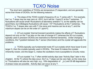
![In all pointed sentences [and tutorials],
some degree of accuracy must be
sacrificed to conciseness.
Samuel Johnson](https://image.slidesharecdn.com/vig-tutorialjan2007-120410082556-phpapp02/85/Vig-tutorial-jan-2007-6-320.jpg)
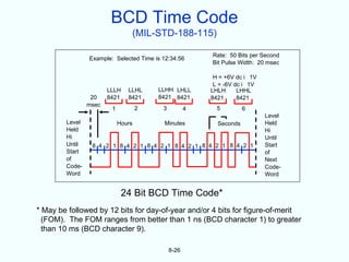
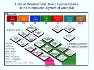
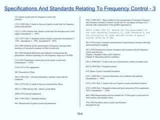
![Utility Fault Location
Zap!
ta tb
Substation Substation
A B
Insulator
Sportsman
X
L
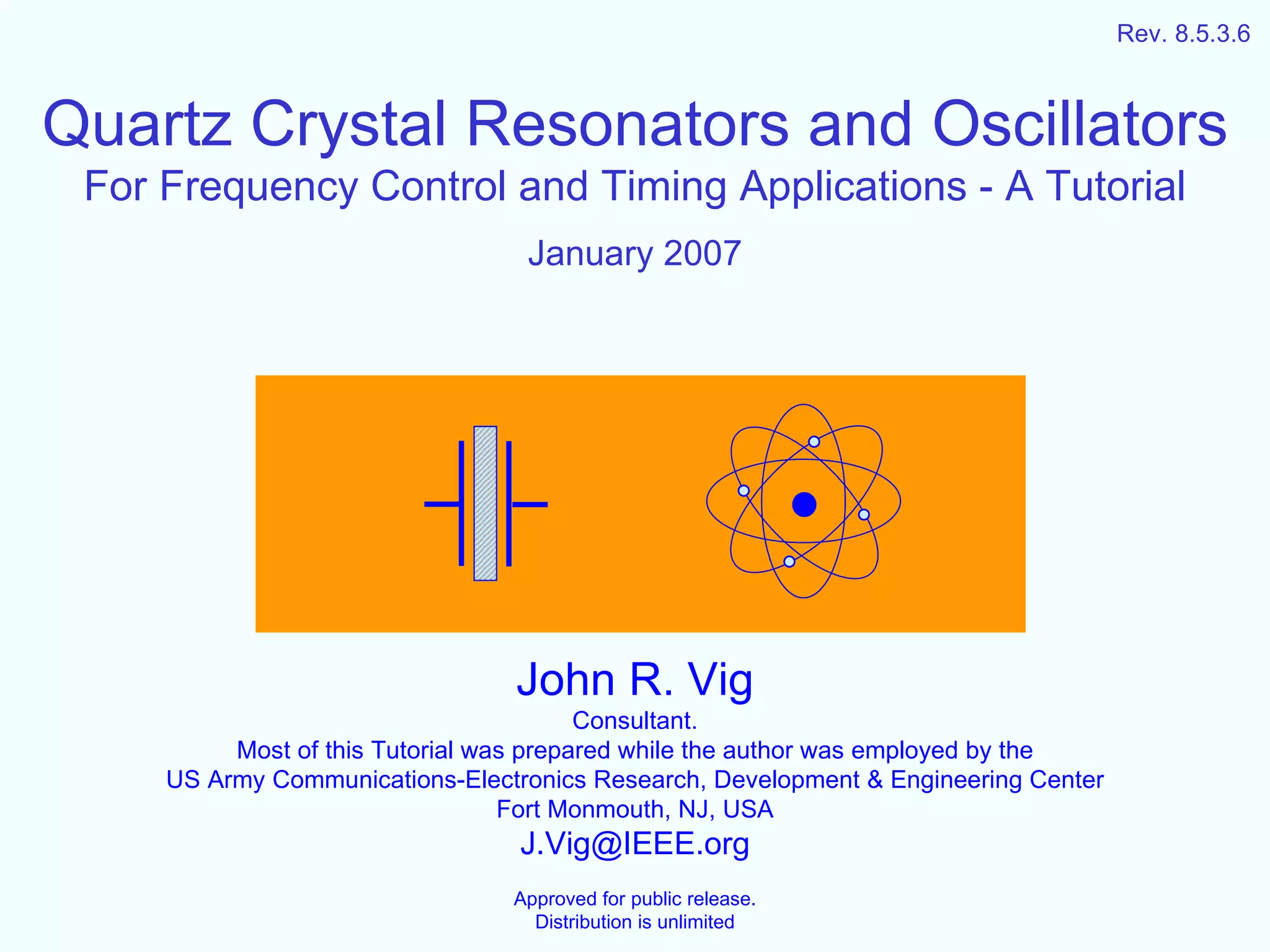
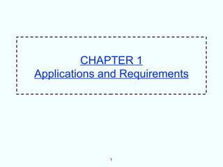
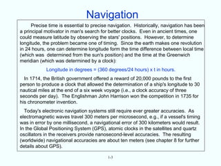
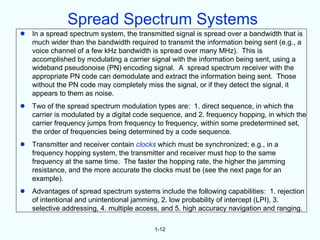
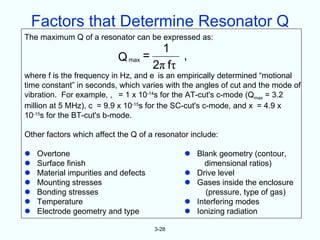
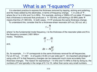
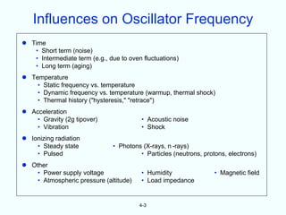
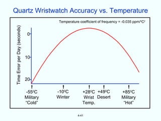
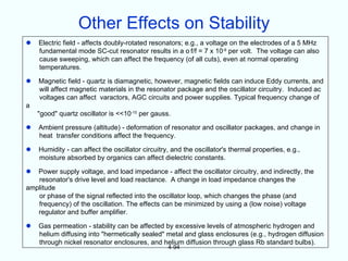
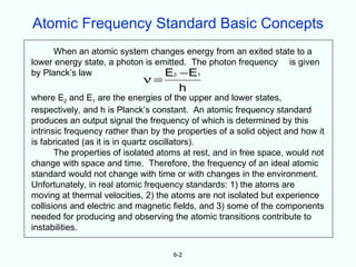
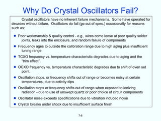
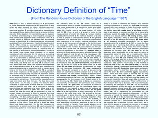
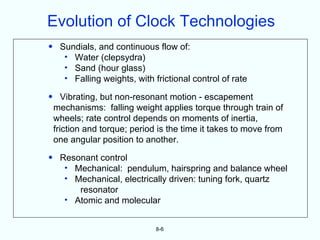
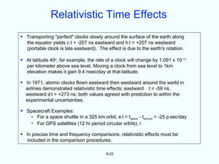
When a fault occurs, e.g., when a "sportsman" shoots out an insulator, a disturbance
propagates down the line. The location of the fault can be determined from the differences
in the times of arrival at the nearest substations:
x=1/2[L - c(tb-ta)] = 1/2[L - c t]
where x = distance of the fault from substation A, L = A to B line length, c = speed of light,
and ta and tb= time of arrival of disturbance at A and B, respectively.
Fault locator error = xterror=1/2(cl error); therefore, if o error e 1 microsecond, then
xerror r 150 meters d 1/2 of high voltage tower spacings, so, the utility company
can send a repair crew directly to the tower that is nearest to the fault.
1-8](https://image.slidesharecdn.com/vig-tutorialjan2007-120410082556-phpapp02/85/Vig-tutorial-jan-2007-15-320.jpg)
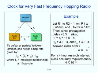

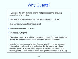


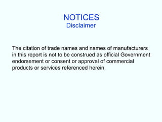
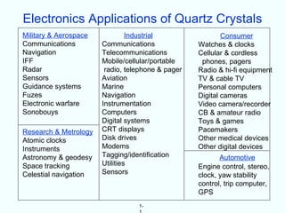
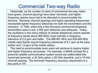
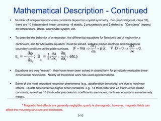
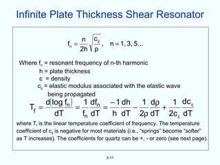
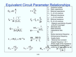
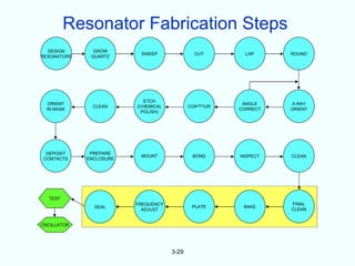
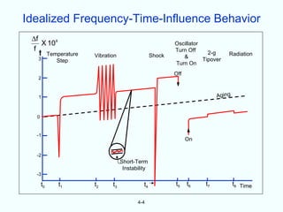
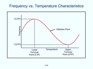
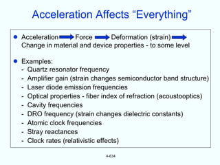
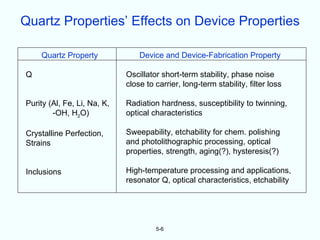
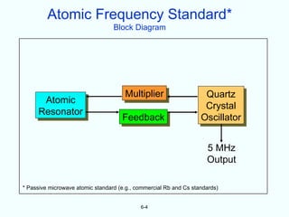
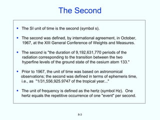
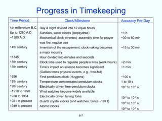
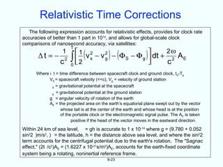
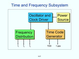
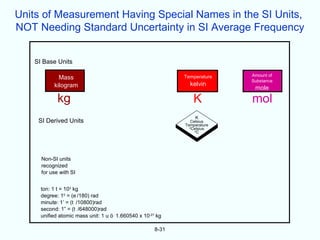
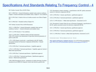
![Mathematical Description of a Quartz Resonator
• In piezoelectric materials, electrical current and voltage are coupled to elastic displacement and stress:
{T} = [c] {S} - [e] {E}
{D} = [e] {S} + [ ] {E}
where {T} = stress tensor, [c] = elastic stiffness matrix, {S} = strain tensor, [e] = piezoelectric matrix
{E} = electric field vector, {D} = electric displacement vector, and [n ] = is the dielectric matrix
• For a linear piezoelectric material16 e11 1e21 2e31
T1
c11 c12 c13 c14 c15 c
c21 c22 c23 c24 c25 c26 2e12 1e22 2e32
S1 • Elasto-electric matrixSfor -E -E
S S S S S
quartz
-E3
T2 S2 1 2 3 4 5 6 1 2
c31 c32 c33 c34 c35 c36 e13 1e23 2e33 S3 T1
T3
c41 c42 c43 c44 c45 c46 e14 1e24 2e34
et
T4 S4 T2
T5 = c51 c52 c53 c54 c55 c56 5e15 1e25 2e35 S5 T3
T6 c61 c62 c63 c64 c65 c66 e16 1e26 2e36 S6 T4
D1 e11 e12 e13 e14 e15 e16 11 1 12 1 13 E1 T5
D2 e21 e22 e23 e24 e25 e26 21 2 22 2 23 E2 T6 CE X
D3 e31 e32 e33 e34 e35 e36 31 3 32 3 33 E3 D1
where
D2
T1 = T11 S1 = S11 6
e S
T2 = T22 S2 = S22 D3 W 2
2
T3 = T33 S3 = S33 LINES JOIN NUMERICAL EQUALITIES 10
EXCEPT FOR COMPLETE RECIPROCITY
T4 = T23 S4 = 2S23 ACROSS PRINCIPAL DIAGONAL
T5 = T13 S5 = 2S13 INDICATES NEGATIVE OF
INDICATES TWICE THE NUMERICAL
T6 = T12 S6 = 2S12 EQUALITIES
X INDICATES 1/2 (c11 - c12)
3-9](https://image.slidesharecdn.com/vig-tutorialjan2007-120410082556-phpapp02/85/Vig-tutorial-jan-2007-61-320.jpg)
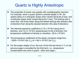
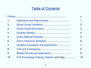
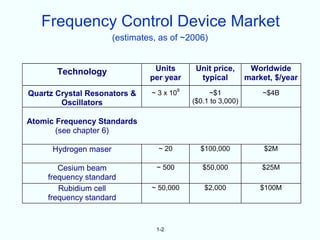
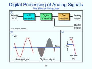
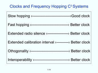
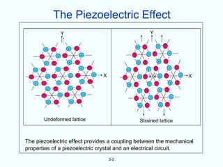
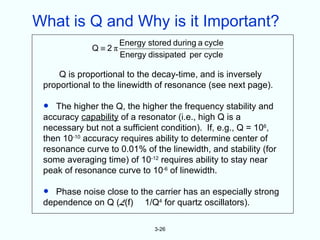
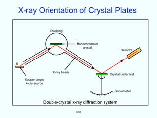
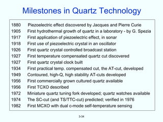
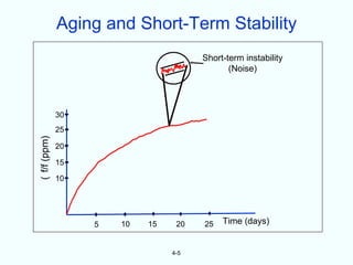
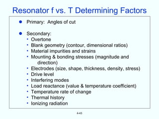
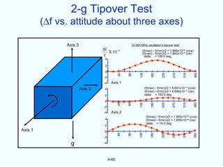
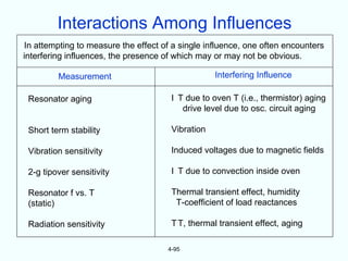
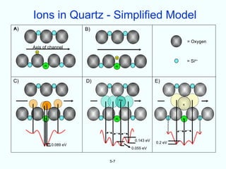
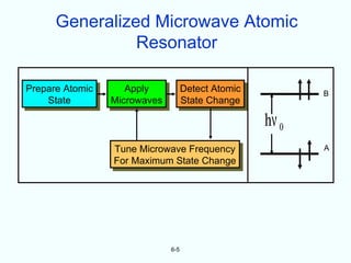
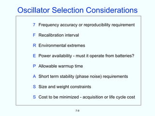
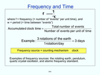
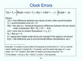
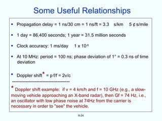
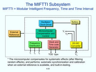
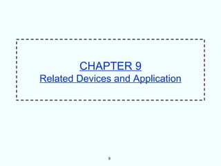
![Resistance vs. Electrode Thickness
AT-cut; f1=12 MHz; polished surfaces; evaporated 1.2 cm (0.490”) diameter silver
electrodes
60
5th
40
RS (Ohms)
20 3rd
Fundamental
0
10 100 1000
−∆f (kHz) [fundamental mode]
3-19](https://image.slidesharecdn.com/vig-tutorialjan2007-120410082556-phpapp02/85/Vig-tutorial-jan-2007-71-320.jpg)
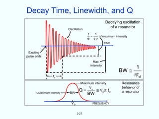
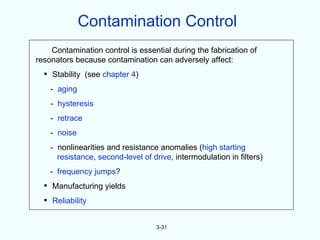
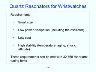
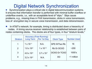
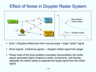
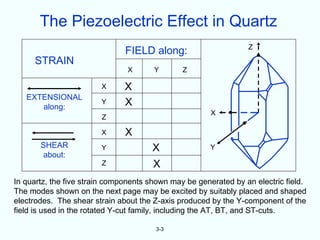
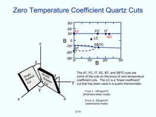
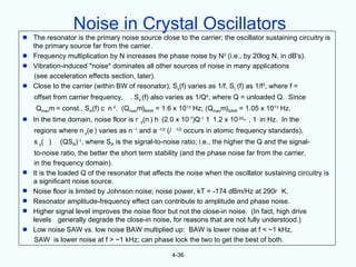
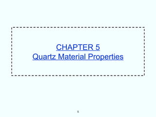
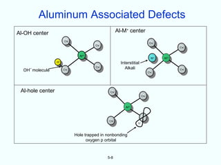
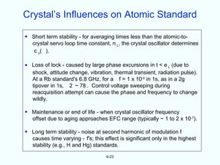
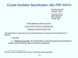
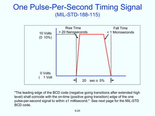
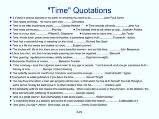
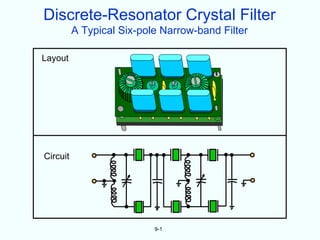
![Short Term Instability (Noise)
Stable Frequency (Ideal Oscillator)
T (t)
1
V
-1
T1 T2 T3
Time
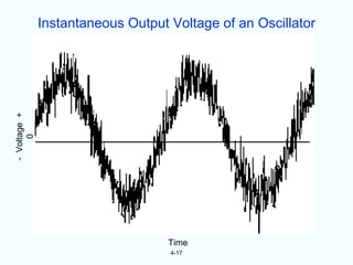
V(t) = V0 sin(2 V 0t) t (t) = 2) ] 0t
Unstable Frequency (Real Oscillator)
1 T (t)
V -1
T1 T2 T3
Time
V(t) =[V0 + + (t)] sin[2r e 0t + (t)] t (t) = 2) ] 0t + = (t)
1 d Φ(t ) 1 dφ(t )
Instantaneous frequency, ν(t) = = ν0 +
2π d t 2π d t
V(t) = Oscillator output voltage, V0 = Nominal peak voltage amplitude
(t) = Amplitude noise, A 0 = Nominal (or "carrier") frequency
(t) = Instantaneous phase, and e (t) = Deviation of phase from nominal (i.e., the ideal)
4-16](https://image.slidesharecdn.com/vig-tutorialjan2007-120410082556-phpapp02/85/Vig-tutorial-jan-2007-109-320.jpg)
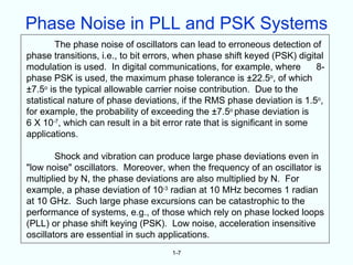
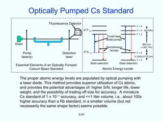
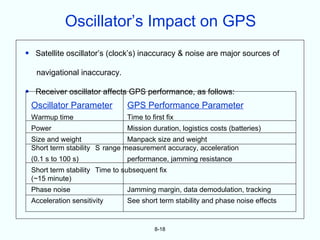
![Impacts of Oscillator Noise
• Limits the ability to determine the current state and the
predictability of oscillators
• Limits syntonization and synchronization accuracy
• Limits receivers' useful dynamic range, channel spacing, and
selectivity; can limit jamming resistance
• Limits radar performance (especially Doppler radar's)
• Causes timing errors [~C y (( )]
• Causes bit errors in digital communication systems
• Limits number of communication system users, as noise from
transmitters interfere with receivers in nearby channels
• Limits navigation accuracy
• Limits ability to lock to narrow-linewidth resonances
• Can cause loss of lock; can limit acquisition/reacquisition
capability in phase-locked-loop systems
4-18](https://image.slidesharecdn.com/vig-tutorialjan2007-120410082556-phpapp02/85/Vig-tutorial-jan-2007-111-320.jpg)
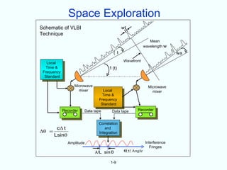
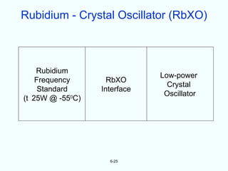
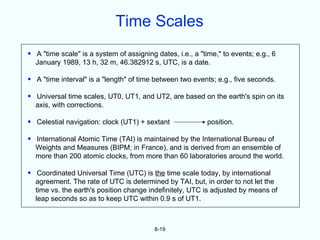
![Short-Term Stability Measures
Measure Symbol
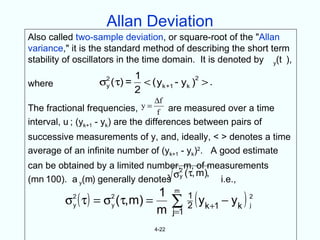
Two-sample deviation, also called “Allan deviation” * y(
Spectral density of phase deviations SS (f)
Spectral density of fractional frequency deviations Sy(f)
Phase noise L(f)*
* Most frequently found on oscillator specification sheets
f2SS (f) = Sy(f); L(f)
2
½ [S( (f)] (per IEEE Std.
1139),
2 ∞
σ ( τ) = ∫ S φ (f)sin4 ( πfτ)df
2
and
y
( πντ) 2 0
Where = averaging time, = carrier frequency, and f = offset or
Fourier frequency, or “frequency from the carrier”.
4-21](https://image.slidesharecdn.com/vig-tutorialjan2007-120410082556-phpapp02/85/Vig-tutorial-jan-2007-114-320.jpg)
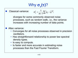
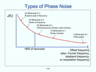
![Pictures of Noise
Plot of z(t) vs. t Sz(f) = h( ff Noise name
f =0 White
= = -1 Flicker
= = -2 Random
walk
= = -3
Plots show fluctuations of a quantity z(t), which can be,e.g., the output of a counter ( f vs. t)
or of a phase detector (o [t] vs. t). The plots show simulated time-domain behaviors
corresponding to the most common (power-law) spectral densities; hc is an amplitude
coefficient. Note: since Sc f = f 2SS , e.g. white frequency noise and random walk of phase
are equivalent.
4-27](https://image.slidesharecdn.com/vig-tutorialjan2007-120410082556-phpapp02/85/Vig-tutorial-jan-2007-120-320.jpg)
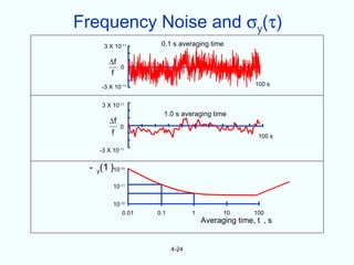
![Spectral Densities
V(t) = [ V0 + ε ( t ) ] sin [ 2 π ν 0 t + φ (t) ]
In the frequency domain, due to the phase deviation, (t), some of
the power is at frequencies other than s 0. The stabilities are
characterized by "spectral densities." The spectral density, SV(f), the
mean-square voltage <V2(t)> in a unit bandwidth centered at f, is not a
good measure of frequency stability because both r
contribute to it, and because it is not uniquely related to frequency
fluctuations (although e (t) is often negligible in precision frequency
sources.)
The spectral densities of phase and fractional-frequency fluctuations,
SS (f) and Sy(f), respectively, are used to measure the stabilities in the
∫
g RMS (t) =g(t) is(f)d f .
S g the
2
frequency domain. The spectral density Sg(f) of a quantity
BW
mean square value of g(t) in a unit bandwidth centered at f. Moreover,
the RMS value of g2 in bandwidth BW is given by
4-28](https://image.slidesharecdn.com/vig-tutorialjan2007-120410082556-phpapp02/85/Vig-tutorial-jan-2007-121-320.jpg)
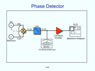
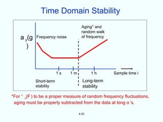
![Phase Noise Measurement
RF Source
V ( t ) = Vo sin[ 2π0 t + Φ( t ) ]
Phase Detector
VV (t) = ke (t)
VV(t)
RF
Voltmeter
Oscilloscope Spectrum Analyzer
S(t) ( (t) in BW of meter
RMS SS (f) vs. f
4-31](https://image.slidesharecdn.com/vig-tutorialjan2007-120410082556-phpapp02/85/Vig-tutorial-jan-2007-124-320.jpg)
![Frequency - Phase - Time Relationships
1 dφ( t ) t
ν( t ) = ν 0 + = " instantaneous" frequency; φ( t ) = φ0 + ∫ 2π[ ν( t' ) − ν 0 ] dt'
2π dt 0
•
ν( t ) − ν 0 φ( t )
y( t ) ≡ = = normalized frequency; φRMS = ∫ S φ ( f ) dt
2
ν0 2πν 0
2
φRMS ν 0
2
Sφ ( f ) = = S y ( f ); L ( f ) ≡ 1/2 S φ ( f ), per IEEE Standard 1139 − 1988
BW f
( )
∞
2
σ ( τ) = 1/2 < y k +1 − y k S φ ( f ) sin 4 ( πfτ) df
2
( πν0 τ) 2 ∫
2
y >=
0
The five common power-law noise processes in precision oscillators are:
S y ( f ) = h2 f 2 + h1f + h0 + h −1f −1 + h −2 f −2
(White PM) (Flicker PM) (White FM) (Flicker FM) (Random-walk FM)
φ( t )
t
Time deviation = x( t ) = ∫ y ( t')dt' =
o
2πν
4-32](https://image.slidesharecdn.com/vig-tutorialjan2007-120410082556-phpapp02/85/Vig-tutorial-jan-2007-125-320.jpg)
![Sφ(f) to SSB Power Ratio Relationship
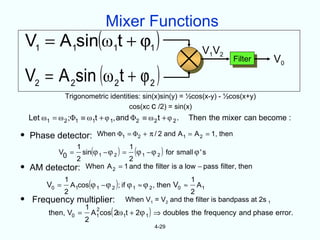
Consider the “simple” case of sinusoidal phase modulation at frequency fm. Then,
. (t) = , o(t)sin(2 fmt), and V(t) = Vocos[2n fct + 2 (t)] = Vocos[2( fct + 2 0(t)sin() fmt)],
where ( o(t)= peak phase excursion, and fc=carrier frequency. Cosine of a sine
function suggests a Bessel function expansion of V(t) into its components at
various frequencies via the identities:
cos( X + Y ) = cosX cosY − sinX sinY
cosXcosY = 1/2[ cos( X + Y ) + cos( X − Y ) ]
− sinXsinY = [ cos( X + Y ) − cos( X − Y ) ]
cos( BsinX ) = J0 (B) + 2 ∑ J2n ( B ) cos( 2nX )
∞
sin( BsinX ) = 2 ∑ J2n+1 ( B ) sin[ ( 2n + 1) X]
n=0
After some messy algebra, SV(f) and S( (f) are as shown on the next page. Then,
V0 J1 [Φ( fm ) ]
2 2
SSB Power Ratio at fm = ∞
V0 J0 [Φ( fm ) ] + 2∑ Ji [Φ( fm ) ]
2 2 2
if Φ( fm ) << 1, then J0 = 1, J1 = 1/2Φ( fm ), Jn = 0 for n > 1, and
i=1
Φ2 ( fm ) S φ ( fm )
SSB Power Ratio = L ( fm ) = =
4 2
4-33](https://image.slidesharecdn.com/vig-tutorialjan2007-120410082556-phpapp02/85/Vig-tutorial-jan-2007-126-320.jpg)
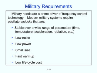
![Sφ(f), Sv(f) and L (f)
Sφ ( f )
Φ( t ) = Φ( fm ) cos( 2πfm t ) Φ2
( fm )
2
0 fm f
V ( t ) = V0cos[ 2πfC t + Φ( fm ) ]
2 2
SV(f) V0 J0
[Φ( fm ) ]
2 2 2
V0 J1
[Φ( fm ) ]
2 2 2
V0 J2
[Φ( fm ) ]
2 2 2
V0 J3
[Φ( fm ) ]
2
fC-3fm fC-2fm fC-fm fC fC+fm fC+2fm fC+3fm
f
V0 J1 [Φ( fm ) ] Sφ( fm )
2 2
SSB Power Ratio = ≅ L ( fm ) ≡
V0 J0 [Φ( fm ) ] + 2∑ J 2 Φ f
∞
2 2 2
i=1 i m
4-34](https://image.slidesharecdn.com/vig-tutorialjan2007-120410082556-phpapp02/85/Vig-tutorial-jan-2007-127-320.jpg)
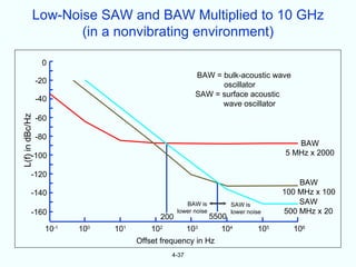
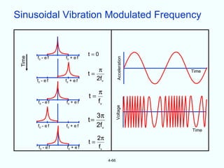
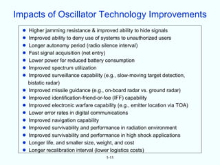
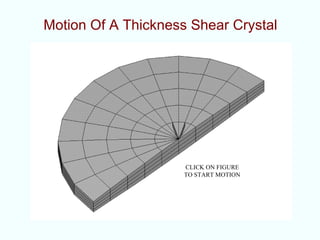
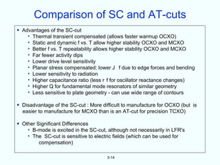
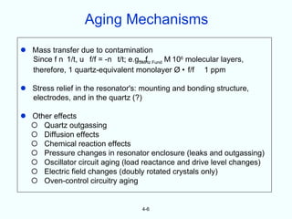
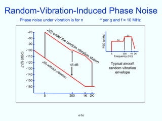
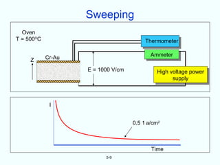
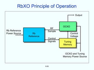
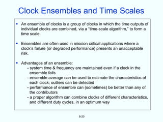
![Random Vibration-Induced Phase Noise
Random vibration’s contribution to phase noise is given by:
Γ • Af0
L ( f ) = 20 log where lAl = [ ( 2)( PSD ) ]
1
2f ,
2
e.g., if = 1 x 10⁻⁹/g and f0 = 10 MHz, then even if the
oscillator is completely noise free at rest, the phase “noise”
i.e., the spectral lines, due solely to a vibration of power
spectral density, PSD = 0.1 g2/Hz will be:
Offset freq., f, in Hz L’(f), in dBc/Hz
1 -53
10 -73
100 -93
1,000 -113
10,000 -133
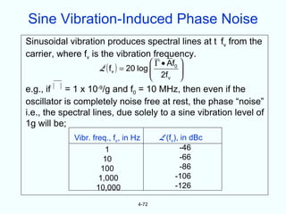
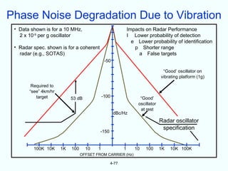
4-73](https://image.slidesharecdn.com/vig-tutorialjan2007-120410082556-phpapp02/85/Vig-tutorial-jan-2007-166-320.jpg)

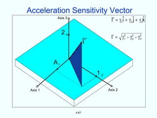
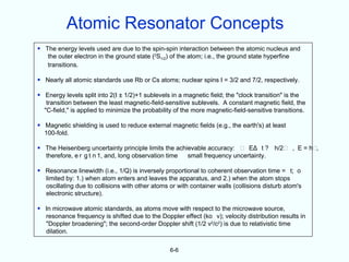
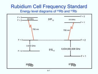
![Hydrogen-Like Atoms
3 MF =
2
Electron 1
spin and 0
Nucleus 2 -1
dipole Electron
Closed
1
electronic
shell N F=2
S
FW 2 3 4 X
S F=1
Electron -1
Nuclear N
spin and MF =
dipole -2 -2
-1
0
-3 1
Hyperfine structure of 87Rb, with nuclear spin I=3/2,
Hydrogen-like (or alkali) R0=b W/h=6,834,682,605 Hz and X=[(- J/J) +
atoms (b I/I)]H0/b W calibrated in units of 2.44 x 10³ Oe.
6-3](https://image.slidesharecdn.com/vig-tutorialjan2007-120410082556-phpapp02/85/Vig-tutorial-jan-2007-212-320.jpg)

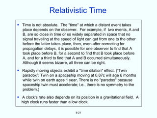
![Calibration With a 1 pps Reference
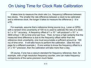
Let A = desired clock rate accuracy after calibration
A' = actual clock rate accuracy
A' = jitter in the 1 pps of the reference clock, rms
= ' = jitter in the 1 pps of the clock being calibrated, rms
t = calibration duration
t t = accumulated time error during calibration
Then, what should be the t for a given set of A, a t, and s t'?
Example: The crystal oscillator in a clock is to be calibrated by
comparing the 1 pps output from the clock with the 1 pps output from a standard. If
A = 1 x 10⁻⁹; = 2
+ ( = ')2]1/2 / 1.2 ) s, and
when A = A', d t = (1 x 10⁻⁹)t n (1.2 ' s)N, and t = (1200N) s. The value of N to be
chosen depends on the statistics of the noise processes, on the confidence level
desired for A' to be A, and on whether one makes measurements every second
or only at the end points. If one measures at the end points only, and the noise is
white phase noise, and the measurement errors are normally distributed, then, with
N = 1, 68% of the calibrations will be within A; with N = 2, and 3, 95% and 99.7%,
respectively, will be within A. One can reduce t by about a factor 2/N3/2 by making
measurements every second; e.g., from 1200 s to 2 x (1200)2/3 = 226 s.
8-14](https://image.slidesharecdn.com/vig-tutorialjan2007-120410082556-phpapp02/85/Vig-tutorial-jan-2007-262-320.jpg)
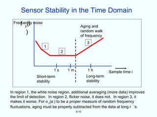


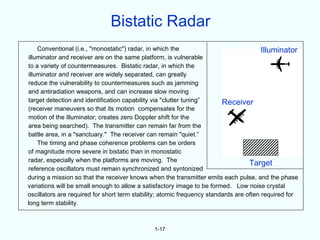
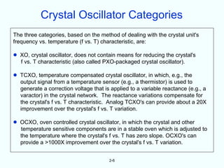
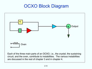
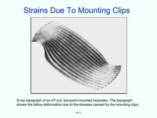
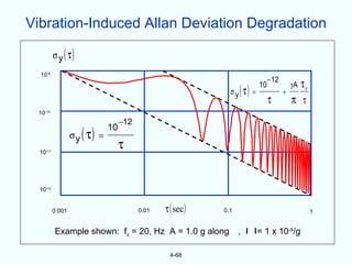
This document provides a tutorial on quartz crystal resonators and oscillators for frequency control and timing applications. It discusses key applications that require precise frequency control, such as navigation, telecommunications, and digital signal processing. Maintaining tight frequency tolerances is increasingly important as the number of users and channel densities increase for technologies like cellular networks. Precise frequency control and timing is essential for applications like GPS navigation systems.


