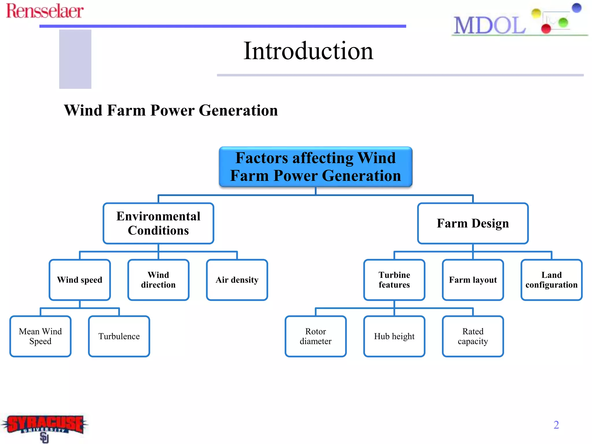
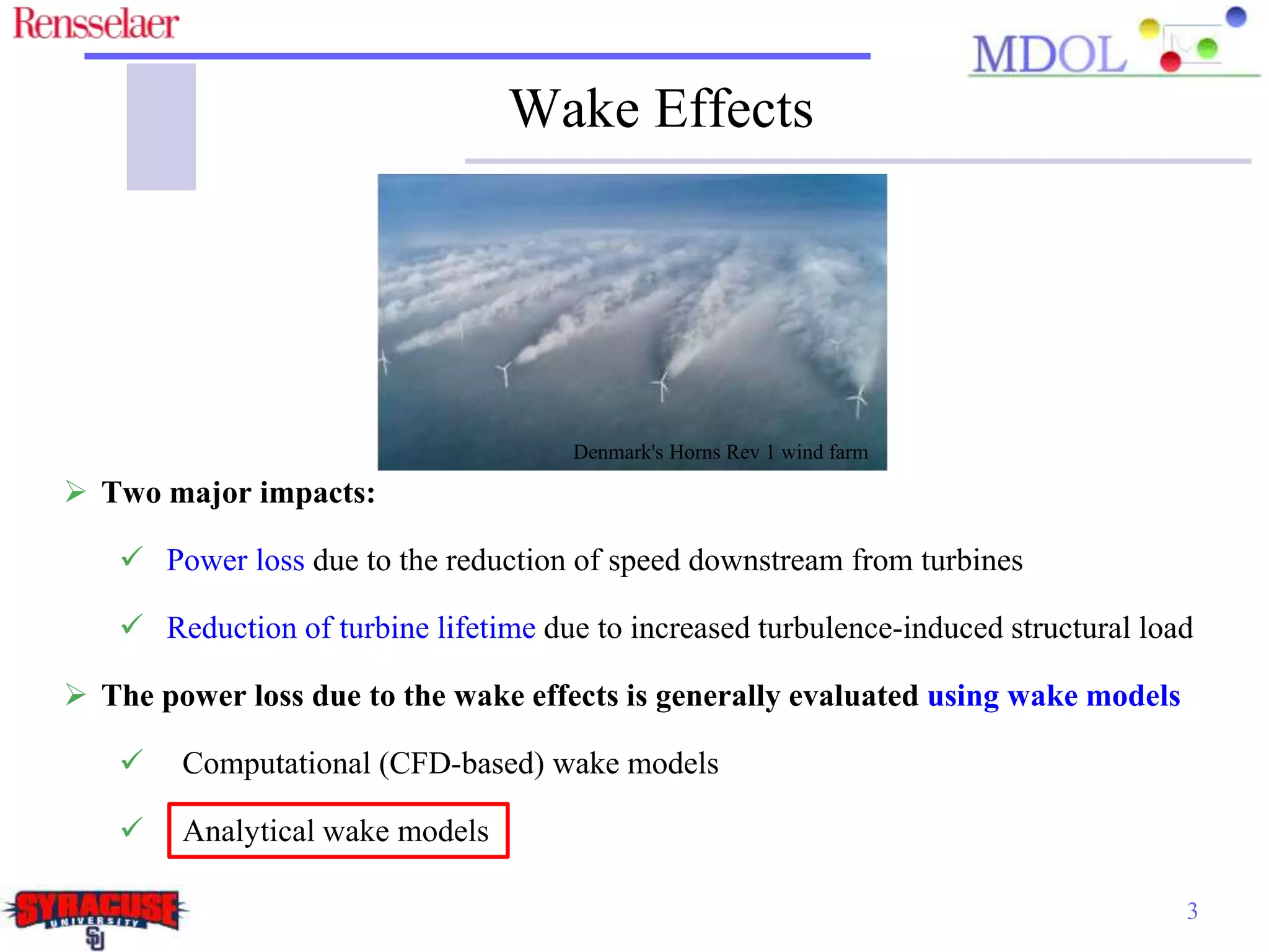
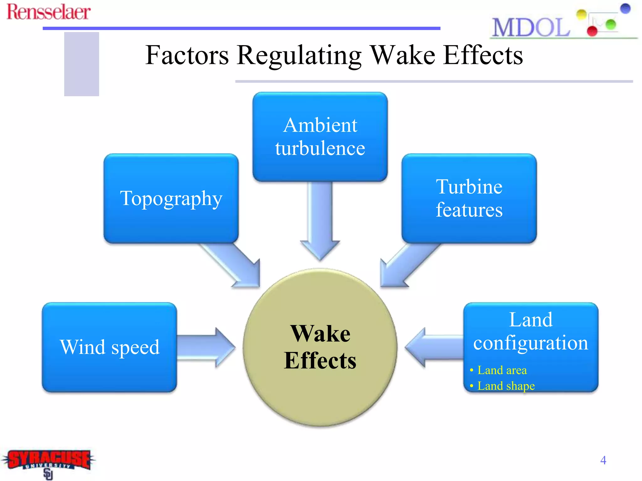
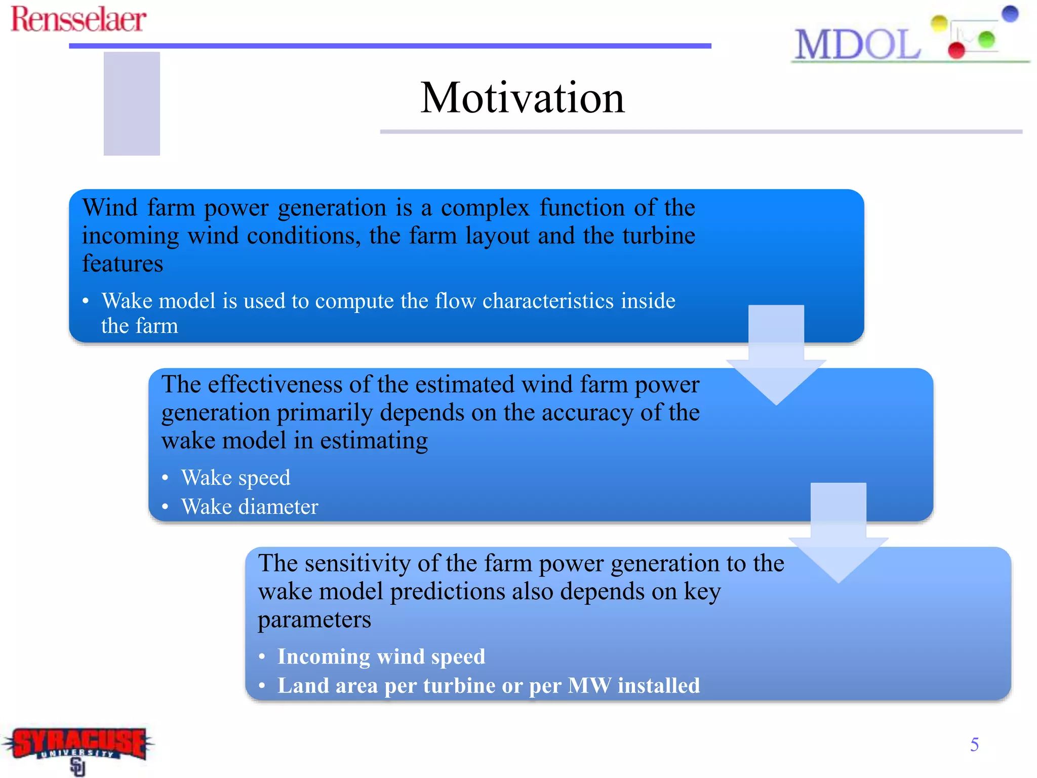
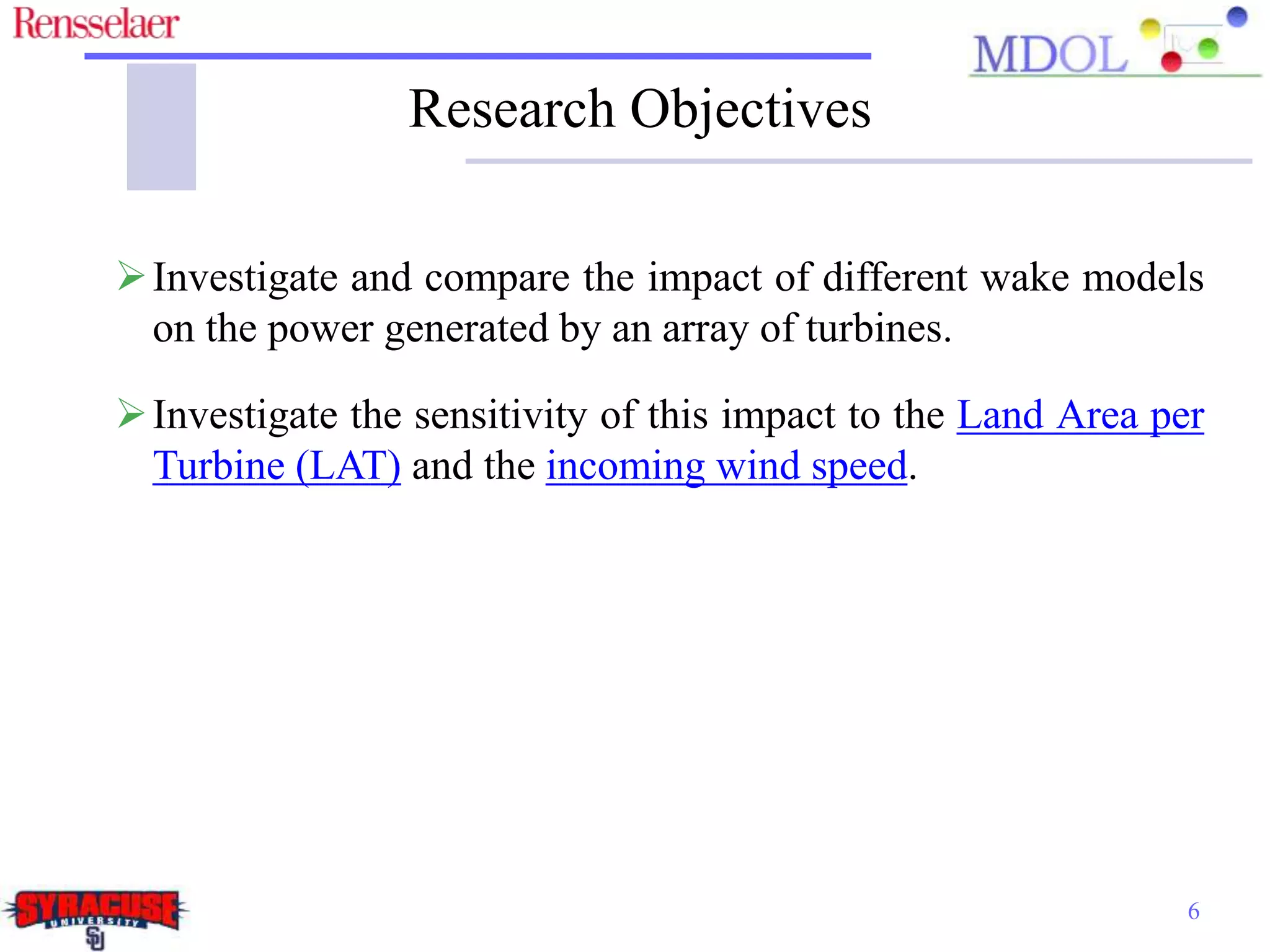
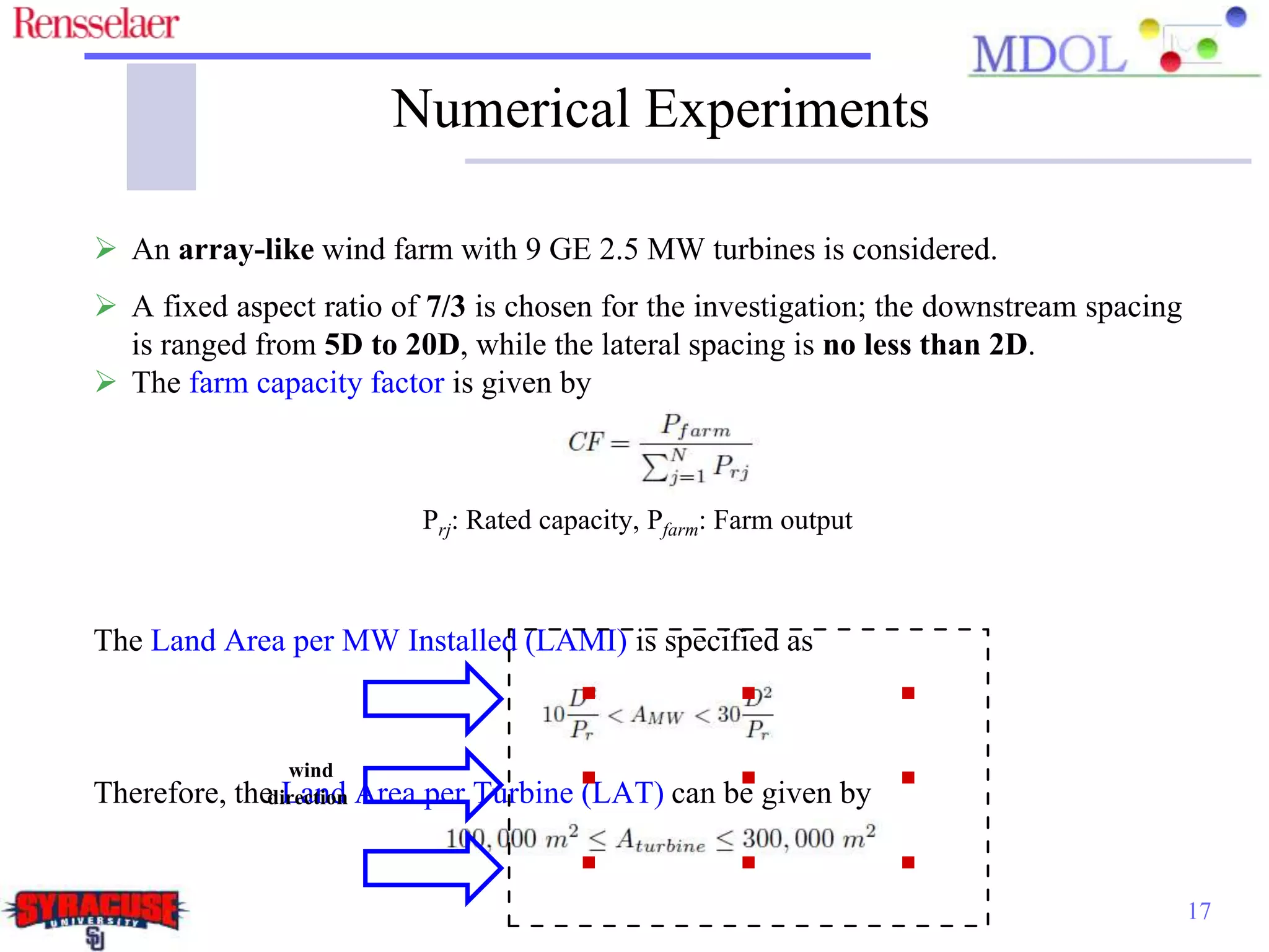
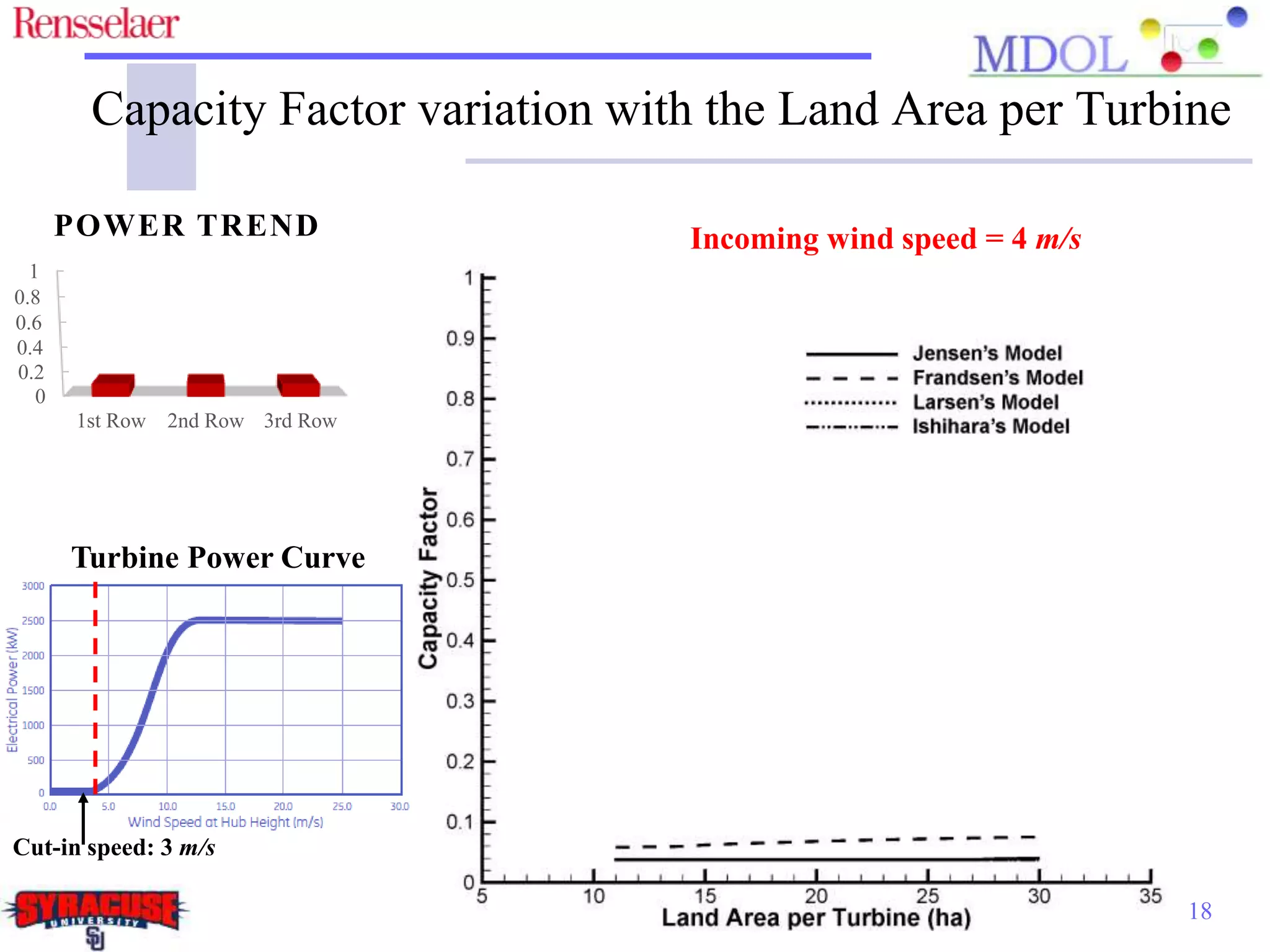
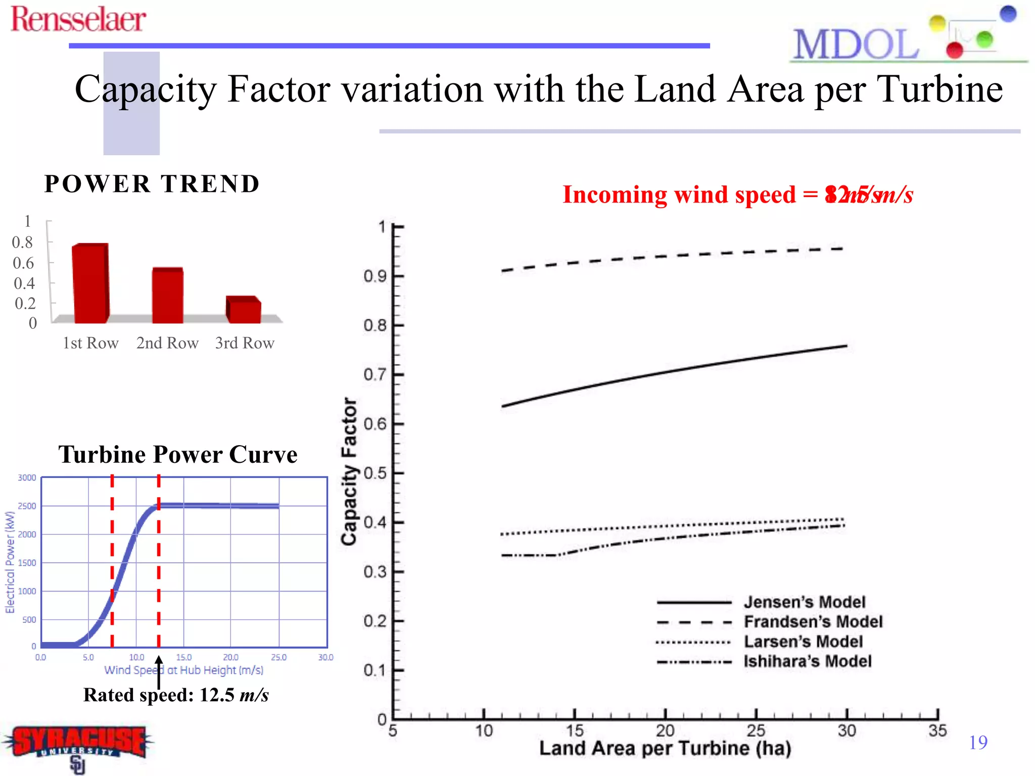
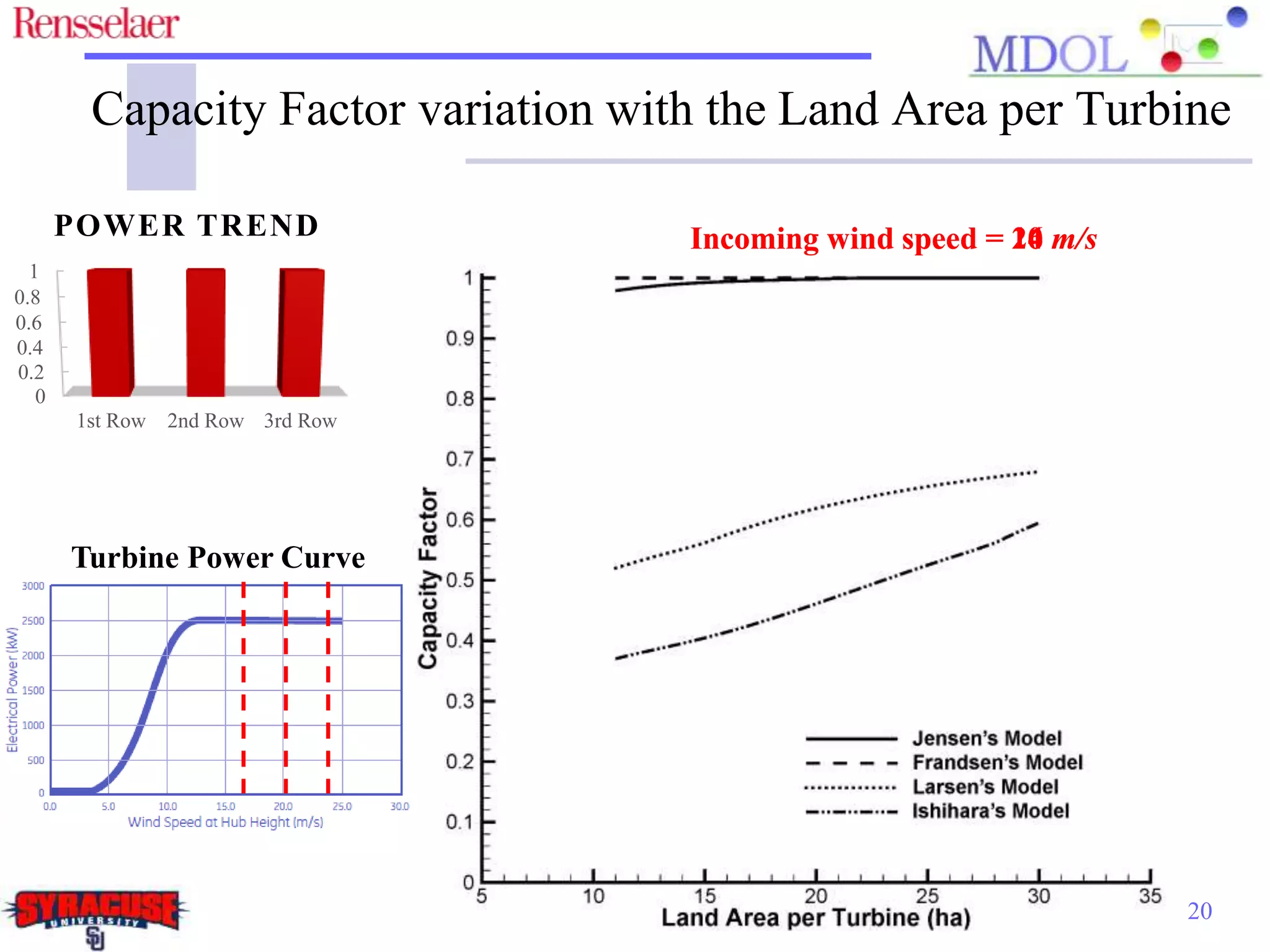
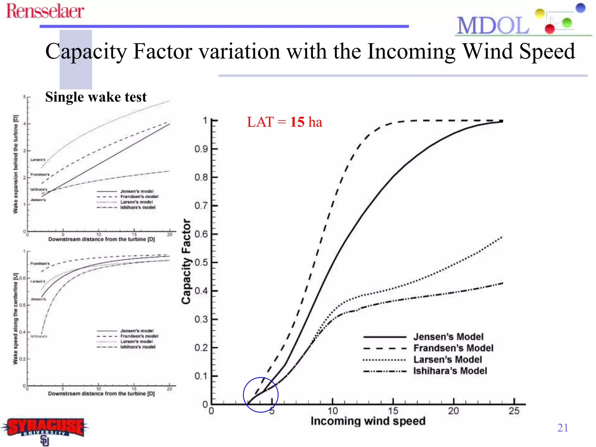
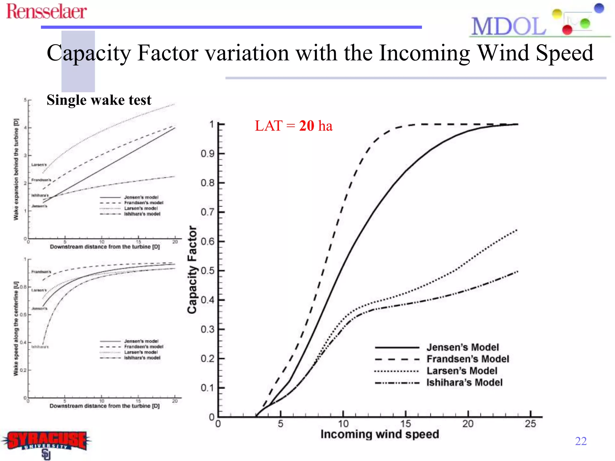
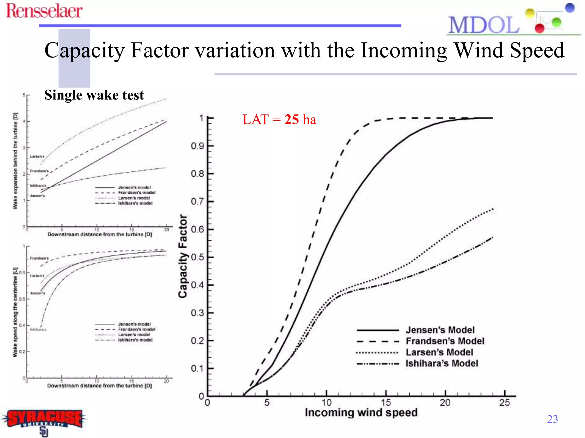
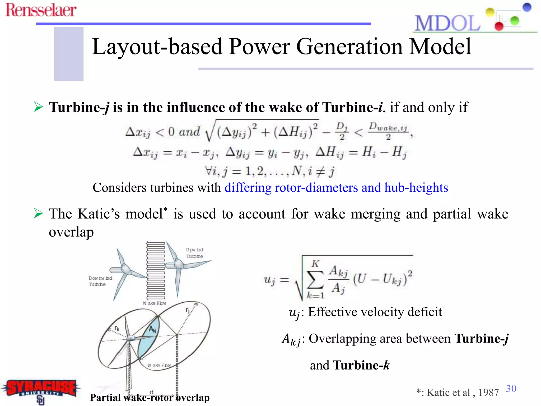
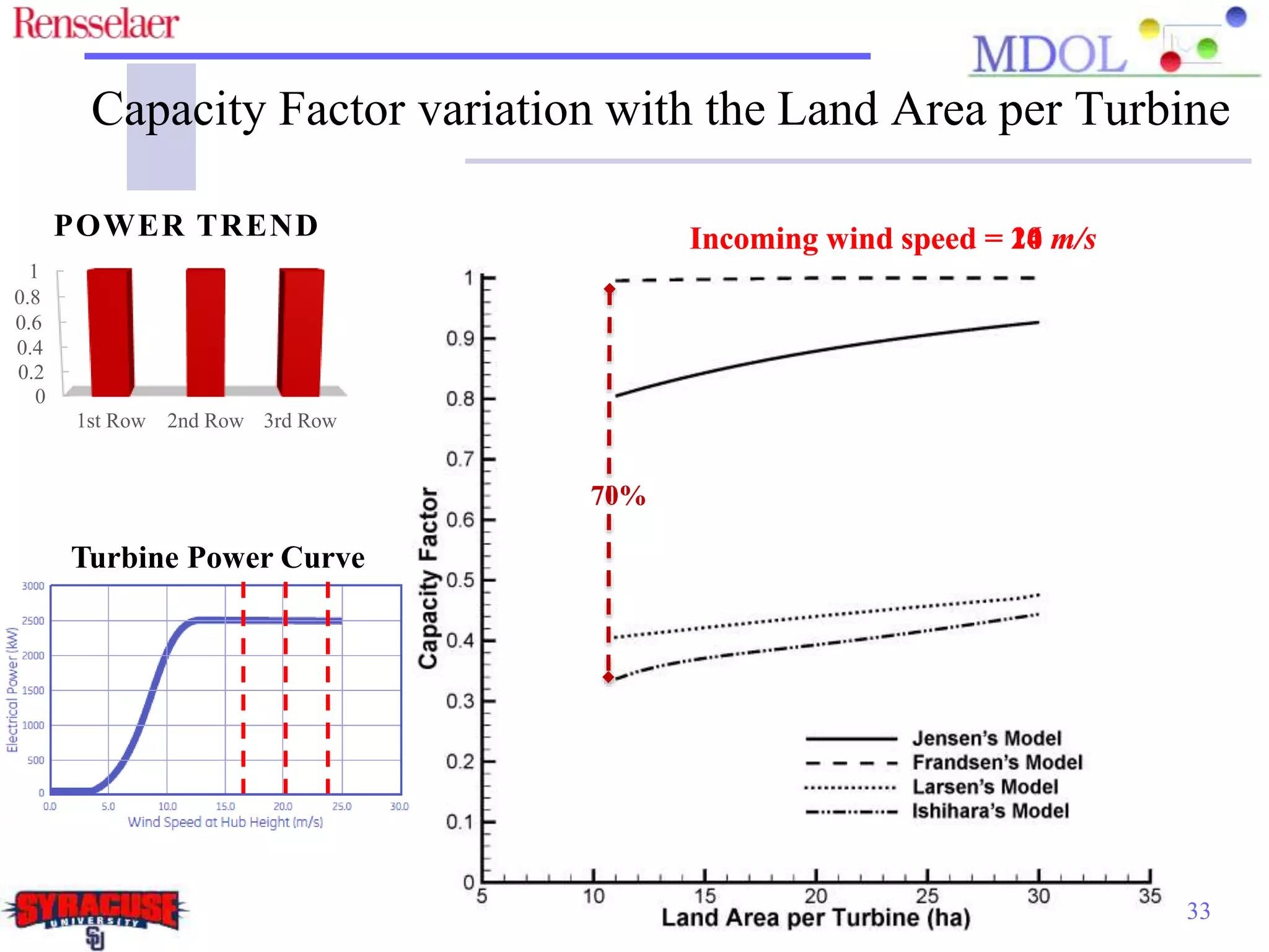
Impact of Different Wake Models on the Estimation
of Wind Farm Power Generation
Weiyang Tong*, Souma Chowdhury#, Jie Zhang#, and Achille Messac*
* Syracuse University, Department of Mechanical and Aerospace Engineering
# Rensselaer Polytechnic Institute, Department of Mechanical, Aerospace, and Nuclear Engineering
14th AIAA/ISSMO Multidisciplinary Analysis and Optimization Conference
17 - 19 Sep 2012
Indianapolis, Indiana
For citations, please refer to the journal version of this paper,
by Tong et al., "Sensitivity of Wind Farm Output to Wind Conditions, Land Configuration, and Installed
Capacity, Under Different Wake Models", J. Mech. Des. 137(6), 061403 (Jun 01, 2015) (11 pages)
Introduction
2
Factors affecting Wind
Farm Power Generation
Environmental
Conditions
Wind speed
Mean Wind
Speed
Turbulence
Wind
direction
Air density
Farm Design
Turbine
features
Rotor
diameter
Hub height
Rated
capacity
Farm layout
Land
configuration
Wind Farm Power Generation
3
Denmark's Horns Rev 1 wind farm
 Two major impacts:
 Power loss due to the reduction of speed downstream from turbines
 Reduction of turbine lifetime due to increased turbulence-induced structural load
 The power loss due to the wake effects is generally evaluated using wake models
 Computational (CFD-based) wake models
 Analytical wake models
Wake Effects
Factors Regulating Wake Effects
Wake
Effects
Wind speed
Topography
Ambient
turbulence
Turbine
features
Land
configuration
• Land area
• Land shape
4
Motivation
5
Wind farm power generation is a complex function of the
incoming wind conditions, the farm layout and the turbine
features
• Wake model is used to compute the flow characteristics inside
the farm
The effectiveness of the estimated wind farm power
generation primarily depends on the accuracy of the
wake model in estimating
• Wake speed
• Wake diameter
The sensitivity of the farm power generation to the
wake model predictions also depends on key
parameters
• Incoming wind speed
• Land area per turbine or per MW installed
Research Objectives
6
Investigate and compare the impact of different wake models
on the power generated by an array of turbines.
Investigate the sensitivity of this impact to the Land Area per
Turbine (LAT) and the incoming wind speed.
Outline
• Standard Wake Models
• Power Generation Modeling
• Comparing Wake Models: Single Wake Test
• Numerical Experiments
• Capacity factor variation with the Land Area per Turbine
• Capacity factor variation with the incoming wind speed
• Concluding Remarks & Future Work
7
Wake Models
8
General inputs and outputs of an analytical wake model
Trujillo, 2005
The wake is fully developed as the shear layer reaches the centerline, i.e., a far wake is
considered in this paper.
Incoming wind speed
Rotor diameter
Hub height
Downstream distance
Radial distance
Ambien turbulence
Near Wake
(2D ~ 5D)
Far Wake
Layout-based Power Generation Model
UWFLO
framework
Wind Distribution
Model
Power Generation
Model
Wind Farm Cost
Model
Optimization
Methodology
9
We use the Power Generation Model developed in the
Unrestricted Wind Farm Layout Optimization (UWFLO) methodology*
*: Chowdhury et al , 2011
Attributes of Major Analytical Wake Models
10
Wake
model
Incoming
wind speed
Downstream
spacing
Radial
spacing
Induction
factor
Rotor
Diameter
Hub
height
Turbulence
intensity
Jensen’s √ √ √ √
Frandsen’s √ √ √ √
Larsen’s √ √ √ √ √ √ √
Ishihara’s √ √ √ √ √ √
 A GE 2.5MW-100m/100m turbine is selected for the
single wake test for each wake model.
 The incoming wind over the rotor area is assumed to
be constant and uniformly distributed; the turbulence
intensity is 10% (onshore*).
 Single wake simulation starts from 2D downstream
distance (far wake)
Inputs to each wake model
*: Mittal, 2011
Specifications Values
Rotor diameter 100 m
Hub height 100 m
Cut-in 3 m/s
Cut-out 25 m/s
Rated speed 12.5 m/s
Wake
model
Jensen’s
Frandsen’s
Larsen’s
Ishihara’s
Far wake
11
Wake expansion,
Velocity deficit,
k: Wake decaying constant
s: Normalized downstream distance from the turbine
CT: Thrust coefficient
Wake model
Incoming
wind speed
Downstream
spacing
Radial
spacing
Induction
factor
Rotor
Diameter
Hub
height
Turbulence
intensity
Jensen’s √ √ √ √
Frandsen’s √ √ √ √
Larsen’s √ √ √ √ √ √ √
Ishihara’s √ √ √ √ √ √
Single Wake Test: Jensen Model
12
Wake expansion,
Velocity deficit*,
𝛼: Initial wake expansion
𝛽: Wake expansion parameter given by
Deff: Effective rotor diameter
*: “+” applies when a ≤ 0.5; “-” applies when a > 0.5.
Wake model
Incoming
wind speed
Downstream
spacing
Radial
spacing
Induction
factor
Rotor
Diameter
Hub
height
Turbulence
intensity
Jensen’s √ √ √ √
Frandsen’s √ √ √ √
Larsen’s √ √ √ √ √ √ √
Ishihara’s √ √ √ √ √ √
Single Wake Test: Frandsen Model
13
Wake expansion,
where constants c1 and x0 are given by,
Velocity deficit,
Wake model
Incoming
wind speed
Downstream
spacing
Radial
spacing
Induction
factor
Rotor
Diameter
Hub
height
Turbulence
intensity
Jensen’s √ √ √ √
Frandsen’s √ √ √ √
Larsen’s √ √ √ √ √ √ √
Ishihara’s √ √ √ √ √ √
Single Wake Test: Larsen Model
Wake radius at a relative distance of 9.5D
Ground Effect
14
Wake expansion,
Velocity deficit,
p is a function related to the turbulence intensity,
Iw is the turbine-generated turbulence intensity,
Wake model
Incoming
wind speed
Downstream
spacing
Radial
spacing
Induction
factor
Rotor
Diameter
Hub
height
Turbulence
intensity
Jensen’s √ √ √ √
Frandsen’s √ √ √ √
Larsen’s √ √ √ √ √ √ √
Ishihara’s √ √ √ √ √ √
Single Wake Test: Ishihara Model
k1, k2, and k3 are respectively set to 0.27, 6.0, and 0.004
15
Single Wake Test: Comparing Wake Growth
 Frandsen model and Larsen model predict
greater wake diameters
 Jensen model has a linear expansion
 The difference between wake diameters
predicted by each model can be as large as
3D, and it can be larger as the downstream
distance increases
3D
16
Single Wake Test: Comparing Wake Speed
 Frandsen model predicts the highest
wake speed
 Ishihara model predicts a relatively
low wake speed; however, as the
downstream distance increases, the
wake recovers fast owing to the
consideration of turbine induced
turbulence in this model
Numerical Experiments
17
 An array-like wind farm with 9 GE 2.5 MW turbines is considered.
 A fixed aspect ratio of 7/3 is chosen for the investigation; the downstream spacing
is ranged from 5D to 20D, while the lateral spacing is no less than 2D.
 The farm capacity factor is given by
Prj: Rated capacity, Pfarm: Farm output
The Land Area per MW Installed (LAMI) is specified as
Therefore, the Land Area per Turbine (LAT) can be given by
wind
direction
Capacity Factor variation with the Land Area per Turbine
18
Incoming wind speed = 4 m/s
Turbine Power Curve
Cut-in speed: 3 m/s
0
0.2
0.4
0.6
0.8
1
1st Row 2nd Row 3rd Row
POWER TREND
19
Incoming wind speed = 8 m/sIncoming wind speed = 12.5 m/s
Capacity Factor variation with the Land Area per Turbine
Rated speed: 12.5 m/s
Turbine Power Curve
0
0.2
0.4
0.6
0.8
1
1st Row 2nd Row 3rd Row
POWER TREND
Turbine Power Curve
20
Incoming wind speed = 16 m/sIncoming wind speed = 20 m/sIncoming wind speed = 24 m/s
Capacity Factor variation with the Land Area per Turbine
0
0.2
0.4
0.6
0.8
1
1st Row 2nd Row 3rd Row
POWER TREND
21
Capacity Factor variation with the Incoming Wind Speed
LAT = 15 ha
Single wake test
22
Capacity Factor variation with the Incoming Wind Speed
LAT = 20 ha
Single wake test
23
Capacity Factor variation with the Incoming Wind Speed
LAT = 25 ha
Single wake test
Single wake test
24
Capacity Factor variation with the Incoming Wind Speed
LAT = 30 ha
Concluding Remarks & Future Work
 The impact of different wake models on the estimation of wind farm power
generation was investigated.
 The sensitivity of using different wake models to the Land Area per Turbine (LAT)
and the incoming wind speed was also investigated.
 A significant difference was observed: in general, Frandsen and Larsen wake models
estimate greater wake diameters, and Frandsen and Jenson wake models estimate
lower wake velocity deficits.
 The maximum difference in the farm capacity factor predicted by different wake
models was as high as 70%.
 Future research can explore the effect of farm-land shape on the wind farm power
generation, when using different wake models.
25
Acknowledgement
• I would like to acknowledge my research adviser
Prof. Achille Messac for his immense help and
support in this research.
• I would also like to thank my colleagues Souma
Chowdhury and Jie Zhang for their valuable
contributions to this paper.
• Support from the NSF Awards is also
acknowledged.
26
Questions
and
Comments
Thank you
28
Layout-based Power Generation Model
This model quantifies the wind farm power generation as a function of
incoming wind speed, farm layout, and turbine features.
 Transformed co-ordinates are evaluated based on wind direction.
 The turbines are ranked in the increasing order of their x-coordinate.
wind
direction
I II III
x
y
0
29
Layout-based Power Generation Model
 In this power generation model, the induction factor is treated as a
function of the incoming wind speed and turbine features:
U: incoming wind speed; P: power generated, given by the power curve
kg, kb: mechanical and electrical efficiencies, Dj: Rotor Diameter, 𝜌: Air density
 A generalized power curve is used to represent the approximate power
response of a particular turbine
𝑈𝑖𝑛, 𝑈 𝑜𝑢𝑡, and 𝑈𝑟: cut-in speed, cut-out speed, and rated speed
𝑃𝑟: Rated capacity, 𝑃𝑛: Polynomial fit for the generalized power curve*
*: Chowdhury et al , 2011
30
Layout-based Power Generation Model
 Turbine-j is in the influence of the wake of Turbine-i, if and only if
Considers turbines with differing rotor-diameters and hub-heights
 The Katic’s model* is used to account for wake merging and partial wake
overlap
𝑢𝑗: Effective velocity deficit
𝐴 𝑘𝑗: Overlapping area between Turbine-j
and Turbine-k
Partial wake-rotor overlap *: Katic et al , 1987
AR = 8/3
31
AR = 8/3
32
Turbine Power Curve
70%
33
Incoming wind speed = 16 m/sIncoming wind speed = 20 m/sIncoming wind speed = 24 m/s
Capacity Factor variation with the Land Area per Turbine
0
0.2
0.4
0.6
0.8
1
1st Row 2nd Row 3rd Row
POWER TREND

Impact of Different Wake Models on the Estimation of Wind Farm Power Generation

  • 1.
    Impact of DifferentWake Models on the Estimation of Wind Farm Power Generation Weiyang Tong*, Souma Chowdhury#, Jie Zhang#, and Achille Messac* * Syracuse University, Department of Mechanical and Aerospace Engineering # Rensselaer Polytechnic Institute, Department of Mechanical, Aerospace, and Nuclear Engineering 14th AIAA/ISSMO Multidisciplinary Analysis and Optimization Conference 17 - 19 Sep 2012 Indianapolis, Indiana For citations, please refer to the journal version of this paper, by Tong et al., "Sensitivity of Wind Farm Output to Wind Conditions, Land Configuration, and Installed Capacity, Under Different Wake Models", J. Mech. Des. 137(6), 061403 (Jun 01, 2015) (11 pages)
  • 2.
    Introduction 2 Factors affecting Wind FarmPower Generation Environmental Conditions Wind speed Mean Wind Speed Turbulence Wind direction Air density Farm Design Turbine features Rotor diameter Hub height Rated capacity Farm layout Land configuration Wind Farm Power Generation
  • 3.
    3 Denmark's Horns Rev1 wind farm  Two major impacts:  Power loss due to the reduction of speed downstream from turbines  Reduction of turbine lifetime due to increased turbulence-induced structural load  The power loss due to the wake effects is generally evaluated using wake models  Computational (CFD-based) wake models  Analytical wake models Wake Effects
  • 4.
    Factors Regulating WakeEffects Wake Effects Wind speed Topography Ambient turbulence Turbine features Land configuration • Land area • Land shape 4
  • 5.
    Motivation 5 Wind farm powergeneration is a complex function of the incoming wind conditions, the farm layout and the turbine features • Wake model is used to compute the flow characteristics inside the farm The effectiveness of the estimated wind farm power generation primarily depends on the accuracy of the wake model in estimating • Wake speed • Wake diameter The sensitivity of the farm power generation to the wake model predictions also depends on key parameters • Incoming wind speed • Land area per turbine or per MW installed
  • 6.
    Research Objectives 6 Investigate andcompare the impact of different wake models on the power generated by an array of turbines. Investigate the sensitivity of this impact to the Land Area per Turbine (LAT) and the incoming wind speed.
  • 7.
    Outline • Standard WakeModels • Power Generation Modeling • Comparing Wake Models: Single Wake Test • Numerical Experiments • Capacity factor variation with the Land Area per Turbine • Capacity factor variation with the incoming wind speed • Concluding Remarks & Future Work 7
  • 8.
    Wake Models 8 General inputsand outputs of an analytical wake model Trujillo, 2005 The wake is fully developed as the shear layer reaches the centerline, i.e., a far wake is considered in this paper. Incoming wind speed Rotor diameter Hub height Downstream distance Radial distance Ambien turbulence Near Wake (2D ~ 5D) Far Wake
  • 9.
    Layout-based Power GenerationModel UWFLO framework Wind Distribution Model Power Generation Model Wind Farm Cost Model Optimization Methodology 9 We use the Power Generation Model developed in the Unrestricted Wind Farm Layout Optimization (UWFLO) methodology* *: Chowdhury et al , 2011
  • 10.
    Attributes of MajorAnalytical Wake Models 10 Wake model Incoming wind speed Downstream spacing Radial spacing Induction factor Rotor Diameter Hub height Turbulence intensity Jensen’s √ √ √ √ Frandsen’s √ √ √ √ Larsen’s √ √ √ √ √ √ √ Ishihara’s √ √ √ √ √ √  A GE 2.5MW-100m/100m turbine is selected for the single wake test for each wake model.  The incoming wind over the rotor area is assumed to be constant and uniformly distributed; the turbulence intensity is 10% (onshore*).  Single wake simulation starts from 2D downstream distance (far wake) Inputs to each wake model *: Mittal, 2011 Specifications Values Rotor diameter 100 m Hub height 100 m Cut-in 3 m/s Cut-out 25 m/s Rated speed 12.5 m/s Wake model Jensen’s Frandsen’s Larsen’s Ishihara’s Far wake
  • 11.
    11 Wake expansion, Velocity deficit, k:Wake decaying constant s: Normalized downstream distance from the turbine CT: Thrust coefficient Wake model Incoming wind speed Downstream spacing Radial spacing Induction factor Rotor Diameter Hub height Turbulence intensity Jensen’s √ √ √ √ Frandsen’s √ √ √ √ Larsen’s √ √ √ √ √ √ √ Ishihara’s √ √ √ √ √ √ Single Wake Test: Jensen Model
  • 12.
    12 Wake expansion, Velocity deficit*, 𝛼:Initial wake expansion 𝛽: Wake expansion parameter given by Deff: Effective rotor diameter *: “+” applies when a ≤ 0.5; “-” applies when a > 0.5. Wake model Incoming wind speed Downstream spacing Radial spacing Induction factor Rotor Diameter Hub height Turbulence intensity Jensen’s √ √ √ √ Frandsen’s √ √ √ √ Larsen’s √ √ √ √ √ √ √ Ishihara’s √ √ √ √ √ √ Single Wake Test: Frandsen Model
  • 13.
    13 Wake expansion, where constantsc1 and x0 are given by, Velocity deficit, Wake model Incoming wind speed Downstream spacing Radial spacing Induction factor Rotor Diameter Hub height Turbulence intensity Jensen’s √ √ √ √ Frandsen’s √ √ √ √ Larsen’s √ √ √ √ √ √ √ Ishihara’s √ √ √ √ √ √ Single Wake Test: Larsen Model Wake radius at a relative distance of 9.5D Ground Effect
  • 14.
    14 Wake expansion, Velocity deficit, pis a function related to the turbulence intensity, Iw is the turbine-generated turbulence intensity, Wake model Incoming wind speed Downstream spacing Radial spacing Induction factor Rotor Diameter Hub height Turbulence intensity Jensen’s √ √ √ √ Frandsen’s √ √ √ √ Larsen’s √ √ √ √ √ √ √ Ishihara’s √ √ √ √ √ √ Single Wake Test: Ishihara Model k1, k2, and k3 are respectively set to 0.27, 6.0, and 0.004
  • 15.
    15 Single Wake Test:Comparing Wake Growth  Frandsen model and Larsen model predict greater wake diameters  Jensen model has a linear expansion  The difference between wake diameters predicted by each model can be as large as 3D, and it can be larger as the downstream distance increases 3D
  • 16.
    16 Single Wake Test:Comparing Wake Speed  Frandsen model predicts the highest wake speed  Ishihara model predicts a relatively low wake speed; however, as the downstream distance increases, the wake recovers fast owing to the consideration of turbine induced turbulence in this model
  • 17.
    Numerical Experiments 17  Anarray-like wind farm with 9 GE 2.5 MW turbines is considered.  A fixed aspect ratio of 7/3 is chosen for the investigation; the downstream spacing is ranged from 5D to 20D, while the lateral spacing is no less than 2D.  The farm capacity factor is given by Prj: Rated capacity, Pfarm: Farm output The Land Area per MW Installed (LAMI) is specified as Therefore, the Land Area per Turbine (LAT) can be given by wind direction
  • 18.
    Capacity Factor variationwith the Land Area per Turbine 18 Incoming wind speed = 4 m/s Turbine Power Curve Cut-in speed: 3 m/s 0 0.2 0.4 0.6 0.8 1 1st Row 2nd Row 3rd Row POWER TREND
  • 19.
    19 Incoming wind speed= 8 m/sIncoming wind speed = 12.5 m/s Capacity Factor variation with the Land Area per Turbine Rated speed: 12.5 m/s Turbine Power Curve 0 0.2 0.4 0.6 0.8 1 1st Row 2nd Row 3rd Row POWER TREND
  • 20.
    Turbine Power Curve 20 Incomingwind speed = 16 m/sIncoming wind speed = 20 m/sIncoming wind speed = 24 m/s Capacity Factor variation with the Land Area per Turbine 0 0.2 0.4 0.6 0.8 1 1st Row 2nd Row 3rd Row POWER TREND
  • 21.
    21 Capacity Factor variationwith the Incoming Wind Speed LAT = 15 ha Single wake test
  • 22.
    22 Capacity Factor variationwith the Incoming Wind Speed LAT = 20 ha Single wake test
  • 23.
    23 Capacity Factor variationwith the Incoming Wind Speed LAT = 25 ha Single wake test
  • 24.
    Single wake test 24 CapacityFactor variation with the Incoming Wind Speed LAT = 30 ha
  • 25.
    Concluding Remarks &Future Work  The impact of different wake models on the estimation of wind farm power generation was investigated.  The sensitivity of using different wake models to the Land Area per Turbine (LAT) and the incoming wind speed was also investigated.  A significant difference was observed: in general, Frandsen and Larsen wake models estimate greater wake diameters, and Frandsen and Jenson wake models estimate lower wake velocity deficits.  The maximum difference in the farm capacity factor predicted by different wake models was as high as 70%.  Future research can explore the effect of farm-land shape on the wind farm power generation, when using different wake models. 25
  • 26.
    Acknowledgement • I wouldlike to acknowledge my research adviser Prof. Achille Messac for his immense help and support in this research. • I would also like to thank my colleagues Souma Chowdhury and Jie Zhang for their valuable contributions to this paper. • Support from the NSF Awards is also acknowledged. 26
  • 27.
  • 28.
    28 Layout-based Power GenerationModel This model quantifies the wind farm power generation as a function of incoming wind speed, farm layout, and turbine features.  Transformed co-ordinates are evaluated based on wind direction.  The turbines are ranked in the increasing order of their x-coordinate. wind direction I II III x y 0
  • 29.
    29 Layout-based Power GenerationModel  In this power generation model, the induction factor is treated as a function of the incoming wind speed and turbine features: U: incoming wind speed; P: power generated, given by the power curve kg, kb: mechanical and electrical efficiencies, Dj: Rotor Diameter, 𝜌: Air density  A generalized power curve is used to represent the approximate power response of a particular turbine 𝑈𝑖𝑛, 𝑈 𝑜𝑢𝑡, and 𝑈𝑟: cut-in speed, cut-out speed, and rated speed 𝑃𝑟: Rated capacity, 𝑃𝑛: Polynomial fit for the generalized power curve* *: Chowdhury et al , 2011
  • 30.
    30 Layout-based Power GenerationModel  Turbine-j is in the influence of the wake of Turbine-i, if and only if Considers turbines with differing rotor-diameters and hub-heights  The Katic’s model* is used to account for wake merging and partial wake overlap 𝑢𝑗: Effective velocity deficit 𝐴 𝑘𝑗: Overlapping area between Turbine-j and Turbine-k Partial wake-rotor overlap *: Katic et al , 1987
  • 31.
  • 32.
  • 33.
    Turbine Power Curve 70% 33 Incomingwind speed = 16 m/sIncoming wind speed = 20 m/sIncoming wind speed = 24 m/s Capacity Factor variation with the Land Area per Turbine 0 0.2 0.4 0.6 0.8 1 1st Row 2nd Row 3rd Row POWER TREND