VHDL Reference - FSM

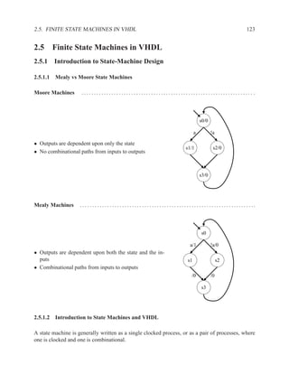
2.5. FINITE STATE MACHINES IN VHDL 123

2.5 Finite State Machines in VHDL
2.5.1 Introduction to State-Machine Design

2.5.1.1 Mealy vs Moore State Machines

Moore Machines ..................................................................... .

s0/0

a !a

• Outputs are dependent upon only the state
s1/1 s2/0
• No combinational paths from inputs to outputs

s3/0

Mealy Machines . . . . . . . . . . . . . . . . . . . . . . . . . . . . . . . . . . . . . . . . . . . . . . . . . . . . . . . . . . . . . . . . . . . . . ..

s0

a/1 !a/0
• Outputs are dependent upon both the state and the in-
puts s1 s2
• Combinational paths from inputs to outputs
/0 /0

s3

2.5.1.2 Introduction to State Machines and VHDL

A state machine is generally written as a single clocked process, or as a pair of processes, where
one is clocked and one is combinational.

124 CHAPTER 2. RTL DESIGN WITH VHDL

Design Decisions ..................................................................... .

• Moore vs Mealy (Sections 2.5.2 and 2.5.3)
• Implicit vs Explicit (Section 2.5.1.3)
• State values in explicit state machines: Enumerated type vs constants (Section 2.5.5.1)
• State values for constants: encoding scheme (binary, gray, one-hot, ...) (Section 2.5.5)

VHDL Constructs for State Machines ..................................................

The following VHDL control constructs are useful to steer the transition from state to state:

• if ... then ... else • loop
• case • next
• for ... loop • exit
• while ... loop

2.5.1.3 Explicit vs Implicit State Machines

There are two broad styles of writing state machines in VHDL: explicit and implicit. “Explicit”
and “implicit” refer to whether there is an explicit state signal in the VHDL code. Explicit state
machines have a state signal in the VHDL code. Implicit state machines do not contain a state
signal. Instead, they use VHDL processes with multiple wait statements to control the execution.
In the explicit style of writing state machines, each process has at most one wait statement. For
the explicit style of writing state machines, there are two sub-categories: “current state” and “cur-
rent+next state”.
In the explicit-current style of writing state machines, the state signal represents the current state
of the machine and the signal is assigned its next value in a clocked process.
In the explicit-current+next style, there is a signal for the current state and another signal for the
next state. The next-state signal is assigned its value in a combinational process or concurrent state-
ment and is dependent upon the current state and the inputs. The current-state signal is assigned
its value in a clocked process and is just a ﬂopped copy of the next-state signal.
For the implicit style of writing state machines, the synthesis program adds an implicit register to
hold the state signal and combinational circuitry to update the state signal. In Synopsys synthesis
tools, the state signal deﬁned by the synthesizer is named multiple wait state reg.
In Mentor Graphics, the state signal is named STATE VAR
We can think of the VHDL code for implicit state machines as having zero state signals, explicit-
current state machines as having one state signal (state), and explicit-current+next state ma-
chines as having two state signals (state and state next).

2.5.2 Implementing a Simple Moore Machine 125

As with all topics in E&CE 327, there are tradeoffs between these different styles of writing state
machines. Most books teach only the explicit-current+next style. This style is the style closest to
the hardware, which means that they are more amenable to optimization through human interven-
tion, rather than relying on a synthesis tool for optimization. The advantage of the implicit style is
that they are concise and readable for control flows consisting of nested loops and branches (e.g.
the type of control flow that appears in software). For control flows that have less structure, it
can be difficult to write an implicit state machine. Very few books or synthesis manuals describe
multiple-wait statement processes, but they are relatively well supported among synthesis tools.

Because implicit state machines are written with loops, if-then-elses, cases, etc. it is difficult to
write some state machines with complicated control flows in an implicit style. The following
example illustrates the point.
a
s0/0 s2/0
!a

!a a
s3/0 s1/1

Note: The terminology of “explicit” and “implicit” is somewhat standard,
in that some descriptions of processes with multiple wait statements describe
the processes as having “implicit state machines”.
There is no standard terminology to distinguish between the two explicit styles:
explicit-current+next and explicit-current.

2.5.2 Implementing a Simple Moore Machine

s0/0
entity simple is
a !a port (
a, clk : in std_logic;
s1/1 s2/0 z : out std_logic
);
end simple;

s3/0


2.5.2.1 Implicit Moore State Machine

Flops 3
architecture moore_implicit_v1a of simple is Gates 2
begin Delay 1 gate
process
begin
z <= ’0’;
wait until rising_edge(clk);
if (a = ’1’) then
z <= ’1’;
else
z <= ’0’;
end if;
z <= ’0’;
end process;
end moore_implicit;

!a
s2/0


2.5.2.2 Explicit Moore with Flopped Output

architecture moore_explicit_v1 of simple is
type state_ty is (s0, s1, s2, s3); Flops 3
signal state : state_ty; Gates 10
begin Delay 3 gates
process (clk)
begin
if rising_edge(clk) then
case state is
when s0 =>
state <= s1;
z <= ’1’;
else
state <= s2;
z <= ’0’;
end if;
when s1 | s2 =>
state <= s3;
z <= ’0’;
when s3 =>
state <= s0;
z <= ’1’;
end case;
end if;
end process;
end moore_explicit_v1;


2.5.2.3 Explicit Moore with Combinational Outputs

Flops 2
architecture moore_explicit_v2 of simple is Gates 7
type state_ty is (s0, s1, s2, s3); Delay 4 gates
signal state : state_ty;
begin
process (clk)
begin
case state is
when s0 =>
state <= s1;
else
state <= s2;
end if;
when s1 | s2 =>
state <= s3;
when s3 =>
state <= s0;
end case;
end if;
end process;
z <= ’1’ when (state = s1)
else ’0’;


2.5.2.4 Explicit-Current+Next Moore with Concurrent Assignment

Flops 2
architecture moore_explicit_v3 of simple is Gates 7
type state_ty is (s0, s1, s2, s3); Delay 4
signal state, state_nxt : state_ty;
begin
process (clk)
begin
state <= state_nxt;
end if;
end process;
state_nxt <= s1 when (state = s0) and (a = ’1’)
else s2 when (state = s0) and (a = ’0’)
else s3 when (state = s1) or (state = s2)
else s0;
else ’0’;

The hardware synthesized from this architecture is the same as that synthesized from moore explicit v2,
which is written in the current-explicit style.


2.5.2.5 Explicit-Current+Next Moore with Combinational Process

architecture moore_explicit_v4 of simple is For this architecture, we
type state_ty is (s0, s1, s2, s3); change the selected assign-
signal state, state_nxt : state_ty; ment to state into a combi-
begin national process using a case
process (clk) statement.
begin
if rising_edge(clk) then Flops 2
state <= state_nxt; Gates 7
end if; Delay 4
end process;
process (state, a) The hardware synthe-
begin sized from this archi-
case state is tecture is the same as
when s0 => that synthesized from
if (a = ’1’) then moore explicit v2 and
state_nxt <= s1; v3.
else
state_nxt <= s2;
end if;
when s1 | s2 =>
state_nxt <= s3;
when s3 =>
state_nxt <= s0;
end case;
end process;
else ’0’;

2.5.3 Implementing a Simple Mealy Machine 131

2.5.3 Implementing a Simple Mealy Machine

Mealy machines have a combinational path from inputs to outputs, which often violates good
coding guidelines for hardware. Thus, Moore machines are much more common. You should
know how to write a Mealy machine if needed, but most of the state machines that you design will
be Moore machines.

This is the same entity as for the simple Moore state machine. The behaviour of the Mealy machine
is the same as the Moore machine, except for the timing relationship between the output (z) and
the input (a).

s0
entity simple is
a/1 !a/0 port (
a, clk : in std_logic;
s1 s2 z : out std_logic
);
/0 /0 end simple;

s3


2.5.3.1 Implicit Mealy State Machine

Note: An implicit Mealy state machine is nonsensical.

In an implicit state machine, we do not have a state signal. But, as the example below illustrates,
to create a Mealy state machine we must have a state signal.

An implicit style is a nonsensical choice for Mealy state machines. Because the output is depen-
dent upon the input in the current clock cycle, the output cannot be a ﬂop. For the output to be
combinational and dependent upon both the current state and the current input, we must create a
state signal that we can read in the assignment to the output. Creating a state signal obviates the
advantages of using an implicit style of state machine.

Flops 4
architecture implicit_mealy of simple is Gates 8
type state_ty is (s0, s1, s2, s3); Delay 2 gates
begin
process
begin
state <= s0;
state <= s1;
else
state <= s2;
end if;
state <= s3;
end process;
z <= ’1’ when (state = s0) and a = ’1’
else ’0;
end mealy_implicit;
/0

!a/0
s2

2.5.3 Implementing a Simple Mealy Machine 133

2.5.3.2 Explicit Mealy State Machine

Flops 2
architecture mealy_explicit of simple is Gates 7
begin
process (clk)
begin
case state is
when s0 =>
state <= s1;
else
state <= s2;
end if;
when s1 | s2 =>
state <= s3;
when others =>
state <= s0;
end case;
end if;
end process;
else ’0’;
end mealy_explicit;


2.5.3.3 Explicit-Current+Next Mealy

Flops 2
architecture mealy_explicit_v2 of simple is Gates 4
signal state, state_nxt : state_ty;
begin
process (clk)
begin
state <= state_nxt;
end if;
end process;
state_nxt <= s1 when (state = s0) and a = ’1’
else s2 when (state = s0) and a = ’0’
else s3 when (state = s1) or (state = s2)
else s0;
else ’0’;
end mealy_explicit_v2;

For the Mealy machine, the explicit-current+next style is smaller than the the explicit-current style.
In contrast, for the Moore machine, the two styles produce exactly the same hardware.

2.5.4 Reset 135

2.5.4 Reset

All circuits should have a reset signal that puts the circuit back into a good initial state. However,
not all ﬂip ﬂops within the circuit need to be reset. In a circuit that has a datapath and a state
machine, the state machine will probably need to be reset, but datapath may not need to be reset.

There are standard ways to add a reset signal to both explicit and implicit state machines.

It is important that reset is tested on every clock cycle, otherwise a reset might not be noticed, or
your circuit will be slow to react to reset and could generate illegal outputs after reset is asserted.

Reset with Implicit State Machine . . .. . . . . .. . . . . .. . . . . .. . . . . .. . . . . .. . . . . .. . . . . . .. . . . . ...

With an implicit state machine, we need to insert a loop in the process and test for reset after each
wait statement.

Here is the implicit Moore machine from section 2.5.2.1 with reset code added in bold.

architecture moore_implicit of simple is
begin
process
begin
init : loop -- outermost loop
z <= ’0’;
next init when (reset = ’1’); -- test for reset
z <= ’1’;
else
z <= ’0’;
end if;
z <= ’0’;
end process;
end moore_implicit;


Reset with Explicit State Machine ......................................................

Reset is often easier to include in an explicit state machine, because we need only put a test for
reset = ’1’ in the clocked process for the state.
The pattern for an explicit-current style of machine is:
process (clk) begin
if reset = ’1’ then
state <= S0;
else
if ... then
state <= ...;
elif ... then
... -- more tests and assignments to state
end if;
end if;
end if;
end process;
Applying this pattern to the explicit Moore machine from section 2.5.2.3 produces:
architecture moore_explicit_v2 of simple is
type state_ty is (s0, s1, s2, s3);
begin
process (clk)
begin
if (reset = ’1’) then
state <= s0;
else
case state is
when s0 =>
state <= s1;
else
state <= s2;
end if;
when s1 | s2 =>
state <= s3;
when s3 =>
state <= s0;
end case;
end if;
end if;
end process;
else ’0’;

2.5.5 State Encoding 137

The pattern for an explicit-current+next style is:

process (clk) begin
if reset = ’1’ then
state_cur <= reset state;
else
state_cur <= state_nxt;
end if;
end if;
end process;

2.5.5 State Encoding

When working with explicit state machines, we must address the issue of state encoding: what
bit-vector value to associate with each state?

With implicit state machines, we do not need to worry about state encoding. The synthesis program
determines the number of states and the encoding for each state.

2.5.5.1 Constants vs Enumerated Type

Using an enumerated type, the synthesis tools chooses the encoding:

type state_ty is (s0, s1, s2, s3);
Using constants, we choose the encoding:

type state_ty is std_logic_vector(1 downto 0);
constant s0 : state_ty := "11";

Providing Encodings for Enumerated Types ............................................

Many synthesizers allow the user to provide hints on how to encode the states, or allow the user to
provide explicitly the desire encoding. These hints are done either through VHDL attributes
or special comments in the code.


Simulation ............................................................................

When doing functional simulation with enumerated types, simulators often display waveforms
with “pretty-printed” values rather than bits (e.g. s0 and s1 rather than 11 and 10). However,
when simulating a design that has been mapped to gates, the enumerated type dissappears and you
are left with just bits. If you don’t know the encoding that the synthesis tool chose, it can be very
difficult to debug the design.

However, this opens you up to potential bugs if the enumerated type you are testing grows to
include more values, which then end up unintentionally executing your when other branch,
rather than having a special branch of their own in the case statement.

Unused Values ....................................................................... .

If the number of values you have in your datatype is not a power of two, then you will have some
unused values that are representable.

For example:

type state_ty is std_logic_vector(2 downto 0);
This type only needs five unique values, but can represent eight different values. What should we
do with the three representable values that we don’t need? The safest thing to do is to code your
design so that if an illegal value is encountered, the machine resets or enters an error state.

2.5.5.2 Encoding Schemes
• Binary: Conventional binary counter.
• One-hot: Exactly one bit is asserted at any time.
• Modified one-hot: Altera’s Quartus synthesizer generates an almost-one-hot encoding where the
bit representing the reset state is inverted. This means that the reset state is all ’O’s and all other
states have two ’1’s: one for the reset state and one for the current state.
• Gray: Transition between adjacent values requires exactly one bit flip.
• Custom: Choose encoding to simplify combinational logic for specific task.

2.6. DATAFLOW DIAGRAMS 139

Tradeoffs in Encoding Schemes ....................................................... .

• Gray is good for low-power applications where consecutive data values typically differ by 1 (e.g.
no random jumps).
• One-hot usually has less combinational logic and runs faster than binary for machines with up
to a dozen or so states. With more than a dozen states, the extra flip-flops required by one-hot
encoding become too expensive.
• Custom is great if you have lots of time and are incredibly intelligent, or have deep insight into
the guts of your design.
Note: Don’t care values When we don’t care what is the value of a signal we
assign the signal ’-’, which is “don’t care” in VHDL. This should allow the
synthesis tool to use whatever value is most helpful in simplifying the Boolean
equations for the signal (e.g. Karnaugh maps). In the past, some groups in
E&CE 327 have used ’-’ quite succesfuly to decrease the area of their design.
However, a few groups found that using ’-’ increased the size of their design,
when they were expecting it to decrease the size. So, if you are tweaking your
design to squeeze out the last few unneeded FPGA cells, pay close attention as
to whether using ’-’ hurts or helps.

2.6 Dataflow Diagrams
2.6.1 Dataflow Diagrams Overview
• Dataflow diagrams are data-dependency graphs where the computation is divided into clock
cycles.
• Purpose:
– Provide a disciplined approach for designing datapath-centric circuits
– Guide the design from algorithm, through high-level models, and finally to register transfer
level code for the datapath and control circuitry.
– Estimate area and performance
– Make tradeoffs between different design options
• Background
– Based on techniques from high-level synthesis tools
– Some similarity between high-level synthesis and software compilation
– Each dataflow diagram corresponds to a basic block in software compiler terminology.

VHDL Reference - FSM

Recommended

Recommended

More Related Content

What's hot

What's hot (20)

Viewers also liked

Viewers also liked (14)

Similar to VHDL Reference - FSM

Similar to VHDL Reference - FSM (20)

Recently uploaded

Recently uploaded (20)

VHDL Reference - FSM