Sigmoid function, Classification Algorithm in Machine Learning, Decision Trees - Structure, working, algorithm, Attribute Selection Measures, Entropy, Information Gain, Gini Index
Machine Learning
Sanjivani RuralEducation Society’s
Sanjivani College of Engineering, Kopargaon-423603
(An Autonomous Institute Affiliated to Savitribai Phule Pune University, Pune)
NAAC ‘A’ Grade Accredited
Department of Information Technology
NBAAccredited-UG Programme
Ms. K. D. Patil
Assistant Professor
2.
Contents - Classification
•Sigmoid function, Classification Algorithm in Machine Learning,
Decision Trees, Ensemble Techniques: Bagging and boosting, Adaboost
and gradient boost, Random Forest, Naïve Bayes Classifier, Support
Vector Machines. Performance Evaluation: Confusion Matrix, Accuracy,
Precision, Recall, AUC-ROC Curves, F-Measure
Machine Learning Department of Information Technology
3.
Course Outcome
• CO3:To apply different classification algorithms for various machine
learning applications.
Machine Learning Department of Information Technology
4.
Sigmoid Function
Machine LearningDepartment of Information Technology
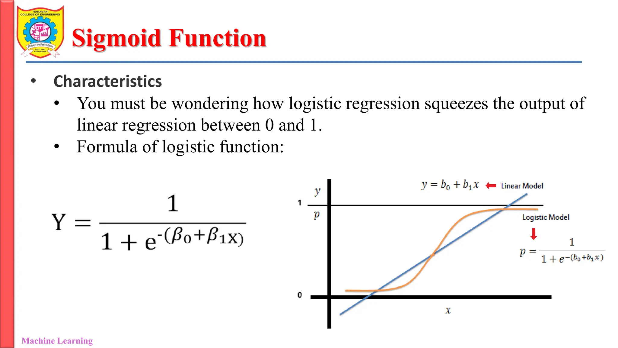
• Characteristics
• You must be wondering how logistic regression squeezes the output of
linear regression between 0 and 1.
• Formula of logistic function:
5.
Sigmoid Function
Machine LearningDepartment of Information Technology
• Characteristics
• S-Shaped Curve: The most prominent characteristic of the sigmoid
function is its S-shaped curve, which makes it suitable for modeling the
probability of binary outcomes.
• Bounded Output: The sigmoid function always produces values
between 0 and 1, which is ideal for representing probabilities.
• Symmetry: The sigmoid function is symmetric around its midpoint at
x=0.5.
• Differentiability: The sigmoid function is differentiable, allowing for the
calculation of gradients necessary for optimization algorithms like
gradient descent.
6.
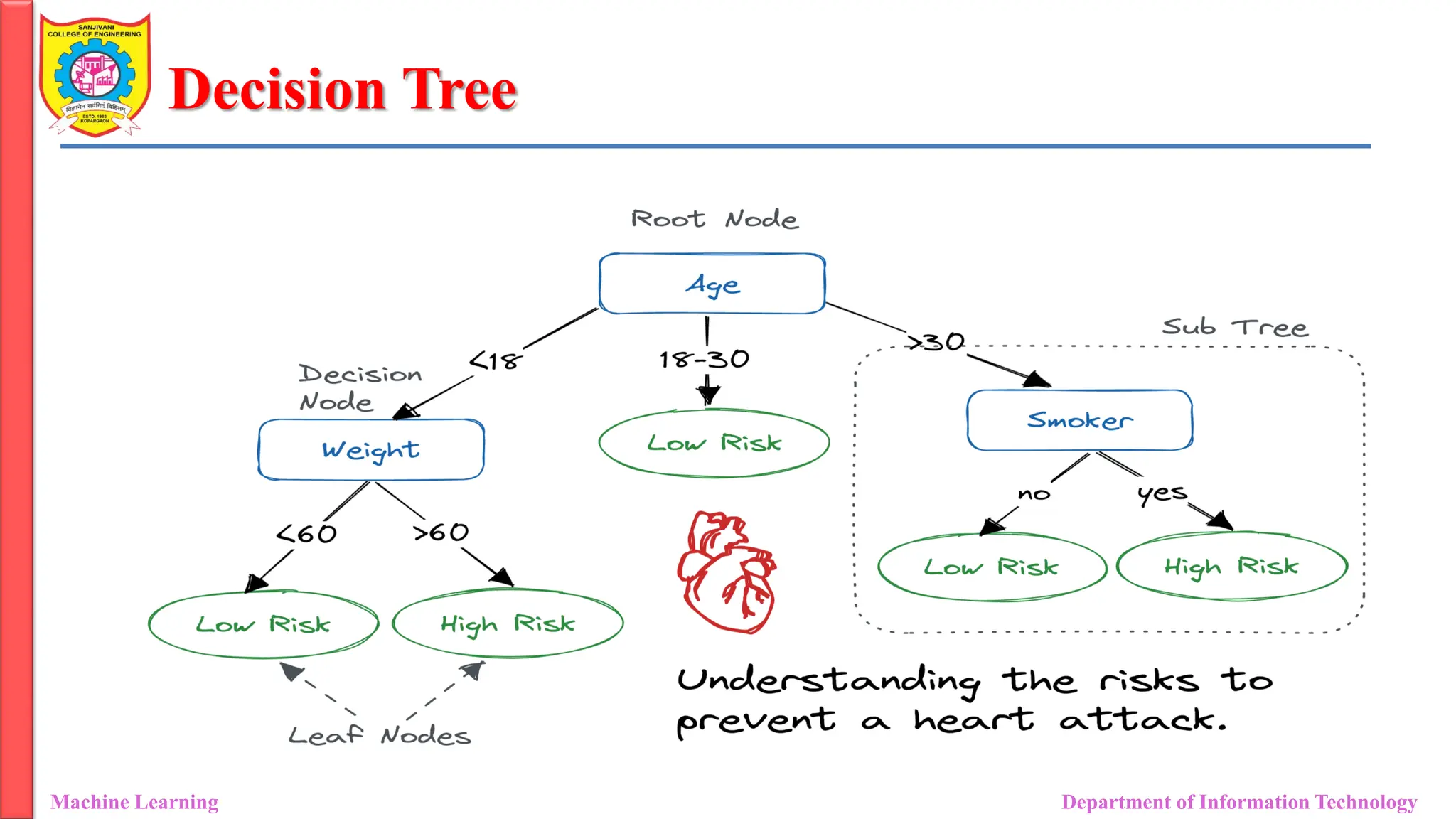
Decision Tree
Machine LearningDepartment of Information Technology
• A decision tree is a non-parametric (not required any assumption)
supervised learning algorithm used for both classification and Regression
problems, but mostly it is preferred for solving Classification problems.
• It has a hierarchical tree structure consisting of a root node, branches,
internal nodes, and leaf nodes.
• The name itself suggests that it uses a flowchart like a tree structure to
show the predictions that result from a series of feature-based splits.
• Internal nodes represent the features of a dataset, branches represent
the decision rules and each leaf node represents the outcome.
• It starts with a root node and ends with a decision made by leaves.
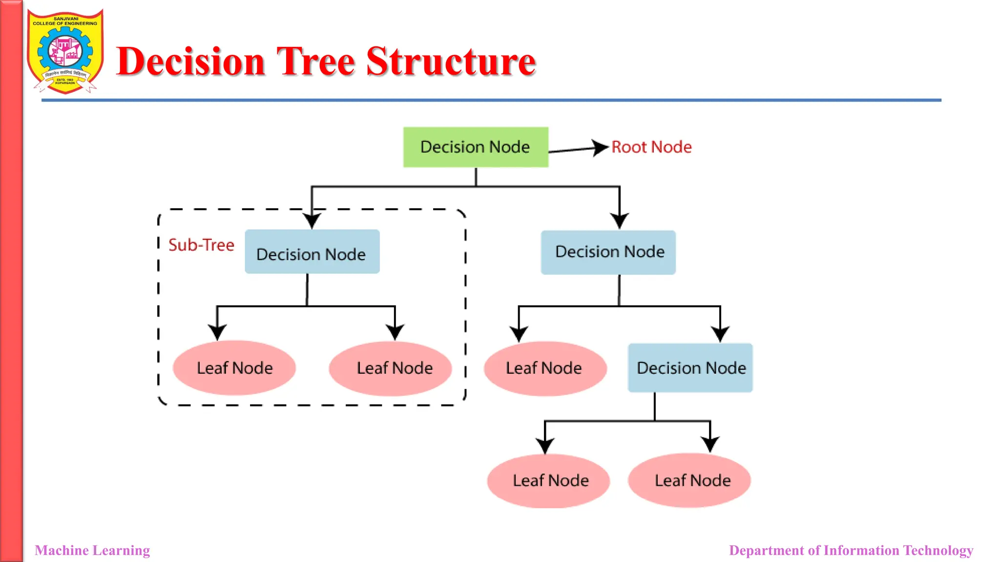
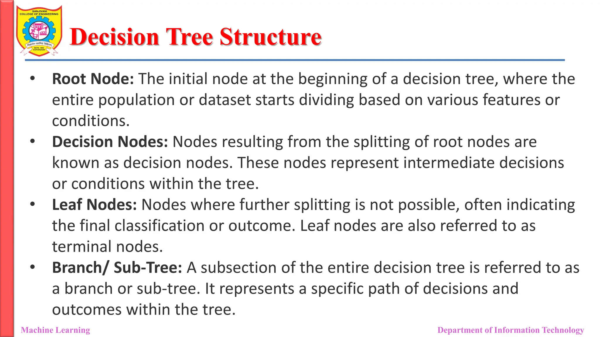
Decision Tree Structure
MachineLearning Department of Information Technology
• Root Node: The initial node at the beginning of a decision tree, where the
entire population or dataset starts dividing based on various features or
conditions.
• Decision Nodes: Nodes resulting from the splitting of root nodes are
known as decision nodes. These nodes represent intermediate decisions
or conditions within the tree.
• Leaf Nodes: Nodes where further splitting is not possible, often indicating
the final classification or outcome. Leaf nodes are also referred to as
terminal nodes.
• Branch/ Sub-Tree: A subsection of the entire decision tree is referred to as
a branch or sub-tree. It represents a specific path of decisions and
outcomes within the tree.
9.
Decision Tree
Machine LearningDepartment of Information Technology
• Pruning: The process of removing or cutting down specific nodes in a
decision tree to prevent over-fitting and simplify the model.
• Parent and Child Node: In a decision tree, a node that is divided into sub
nodes is known as a parent node, and the sub-nodes emerging from it are
referred to as child nodes.
• The parent node represents a decision or condition, while the child nodes
represent the potential outcomes or further decisions based on that
condition.
10.
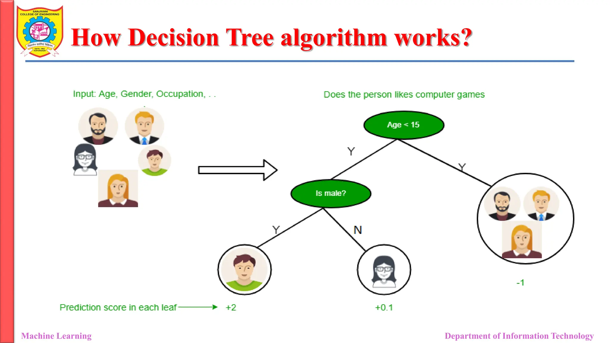
How Decision Treealgorithm works?
Machine Learning Department of Information Technology
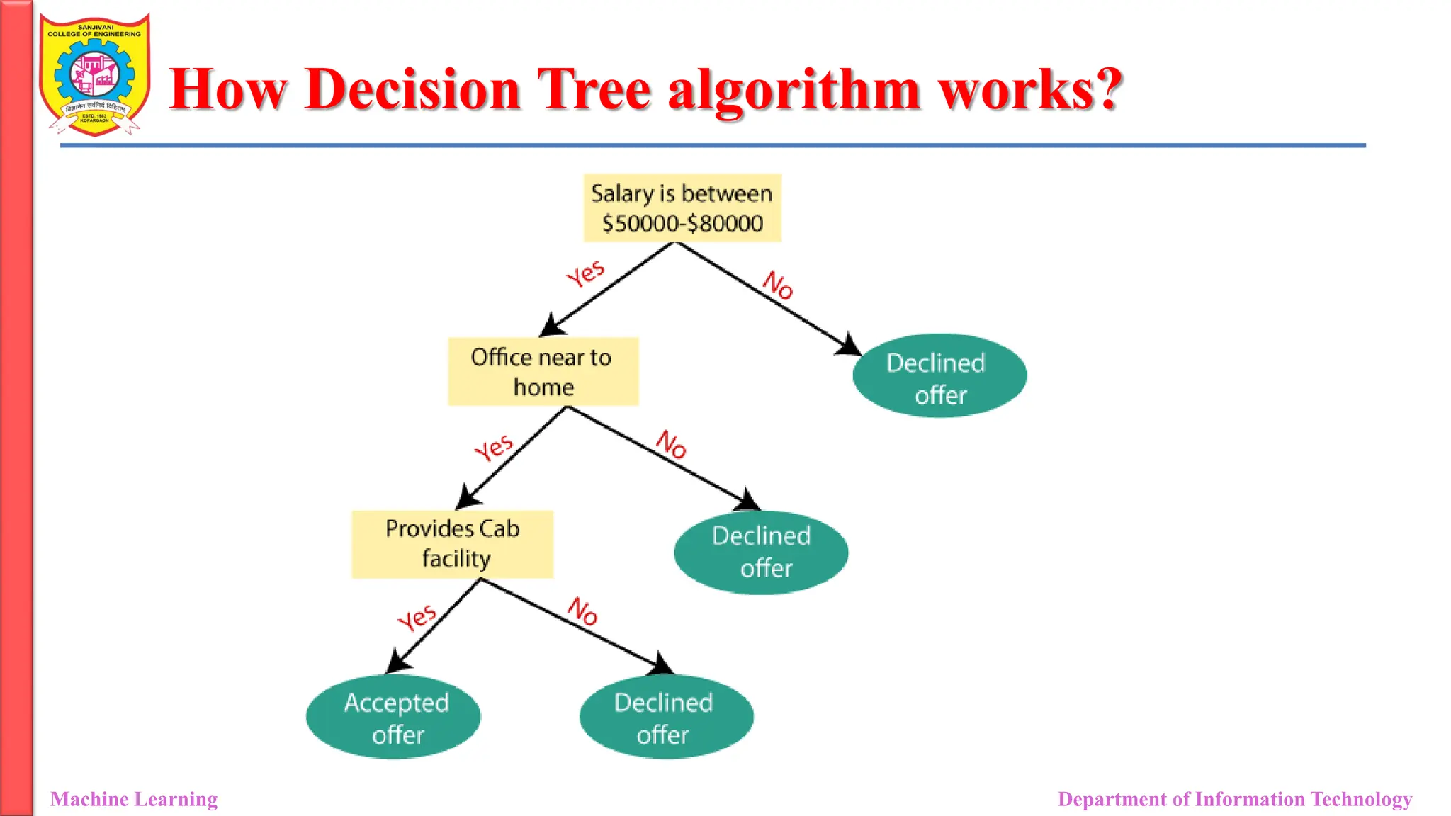
• Starting at the Root: The algorithm begins at the top, called the “root
node,” representing the entire dataset.
• Asking the Best Questions: It looks for the most important feature or
question that splits the data into the most distinct groups. This is like
asking a question at a fork in the tree.
• Branching Out: Based on the answer to that question, it divides the data
into smaller subsets, creating new branches. Each branch represents a
possible route through the tree.
• Repeating the Process: The algorithm continues asking questions and
splitting the data at each branch until it reaches the final “leaf nodes,”
representing the predicted outcomes or classifications.
11.
How Decision Treealgorithm works?
Machine Learning Department of Information Technology
12.
How Decision Treealgorithm works?
Machine Learning Department of Information Technology
Decision Tree Assumptions
MachineLearning Department of Information Technology
• Binary Splits: Decision trees typically make binary splits, meaning each
node divides the data into two subsets based on a single feature or
condition. This assumes that each decision can be represented as a binary
choice.
• Recursive Partitioning: Decision trees use a recursive partitioning process,
where each node is divided into child nodes, and this process continues
until a stopping criterion is met. This assumes that data can be effectively
subdivided into smaller, more manageable subsets.
• Feature Independence: Decision trees often assume that the features
used for splitting nodes are independent. In practice, feature
independence may not hold, but decision trees can still perform well if
features are correlated.
15.
Decision Tree Assumptions
MachineLearning Department of Information Technology
• Top-Down Greedy Approach: Decision trees are constructed using a top
down, greedy approach, where each split is chosen to maximize
information gain or minimize impurity at the current node. This may not
always result in the globally optimal tree.
• Categorical and Numerical Features: Decision trees can handle both
categorical and numerical features. However, they may require different
splitting strategies for each type.
• Impurity Measures: Decision trees use impurity measures such as Gini
impurity or entropy to evaluate how well a split separates classes. The
choice of impurity measure can impact tree construction.
16.
Decision Tree Assumptions
MachineLearning Department of Information Technology
• No Missing Values: Decision trees assume that there are no missing values
in the dataset or that missing values have been appropriately handled
through imputation or other methods.
• Equal Importance of Features: Decision trees may assume equal
importance for all features unless feature scaling or weighting is applied to
emphasize certain features.
• No Outliers: Decision trees are sensitive to outliers, and extreme values
can influence their construction. Pre-processing or robust methods may
be needed to handle outliers effectively.
17.
Decision Tree AttributeSelection Measures
(ASM)
Machine Learning Department of Information Technology
• While implementing a Decision tree, the main issue arises that how to
select the best attribute for the root node and for sub-nodes.
• So, to solve such problems there is a technique which is called as Attribute
Selection Measure or ASM.
• By this measurement, we can easily select the best attribute for the nodes
of the tree.
• Attribute selection measure is a heuristic for selecting the splitting
criterion that partitions data in the best possible manner
• There are two popular techniques for ASM, which are:
• Entropy and Information Gain
• Gini Index
18.
Decision Tree AttributeSelection Measures
(ASM)
Machine Learning Department of Information Technology
• Entropy and Information Gain:
• Entropy is nothing but the uncertainty in our dataset or measure of
disorder.
• Entropy is a measure of the randomness in the information being
processed (how much variance a data has).
• The higher the entropy, the harder it is to draw any conclusions from
that information.
• It calculates how much information a feature provides us about a
class.
19.
Decision Tree AttributeSelection Measures
(ASM)
Machine Learning Department of Information Technology
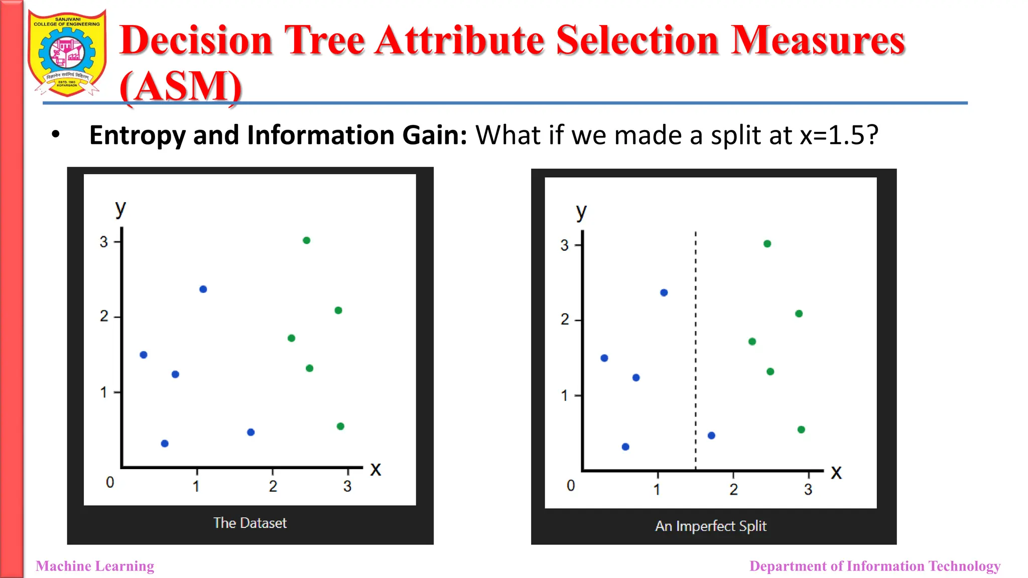
• Entropy and Information Gain: What if we made a split at x=1.5?
20.
Decision Tree AttributeSelection Measures
(ASM)
Machine Learning Department of Information Technology
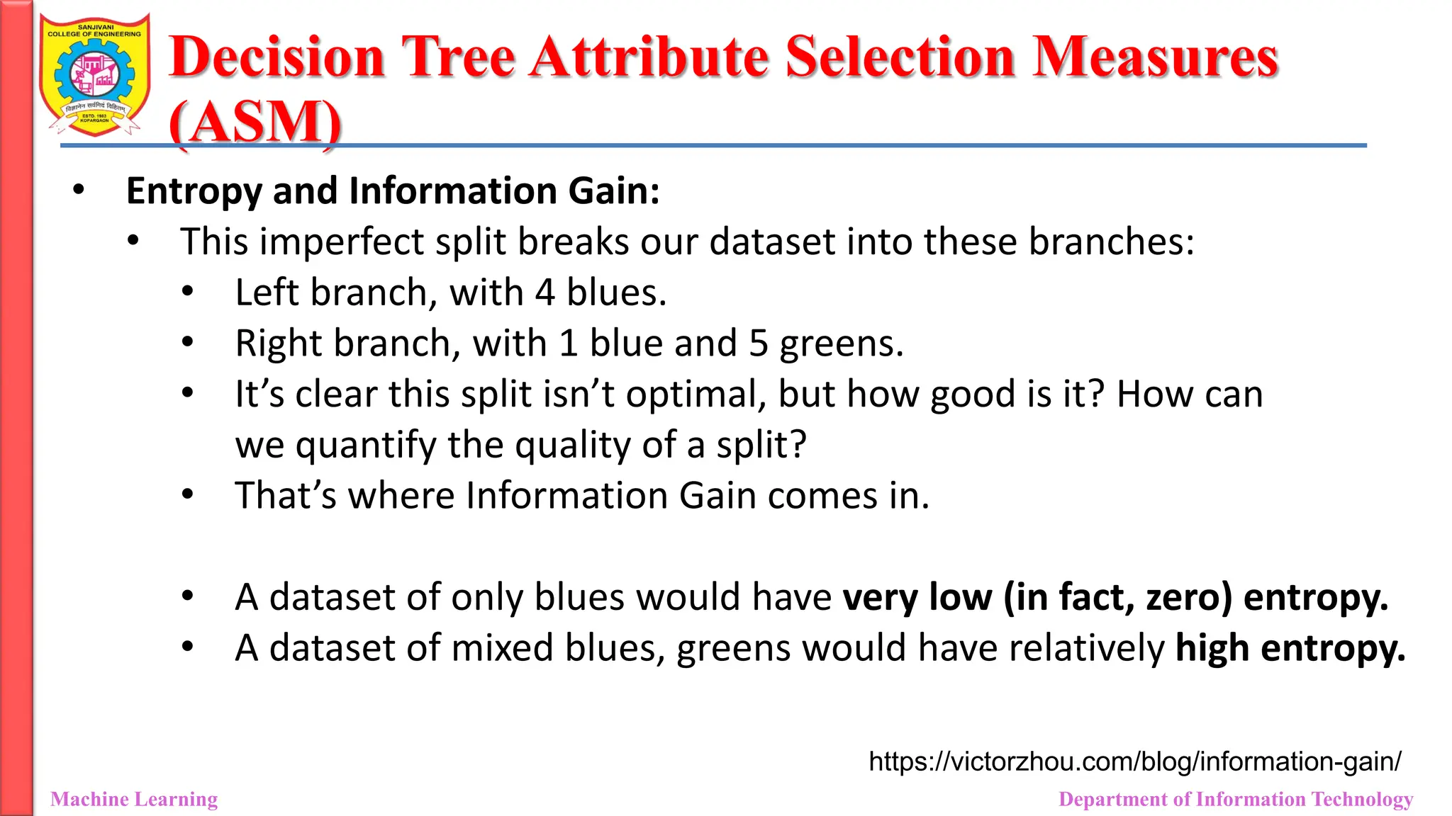
• Entropy and Information Gain:
• This imperfect split breaks our dataset into these branches:
• Left branch, with 4 blues.
• Right branch, with 1 blue and 5 greens.
• It’s clear this split isn’t optimal, but how good is it? How can
we quantify the quality of a split?
• That’s where Information Gain comes in.
• A dataset of only blues would have very low (in fact, zero) entropy.
• A dataset of mixed blues, greens would have relatively high entropy.
https://victorzhou.com/blog/information-gain/
21.
Decision Tree AttributeSelection Measures
(ASM)
Machine Learning Department of Information Technology
• Entropy and Information Gain:
• Thus, a node with more variable composition, such as 2 Pass and 2 Fail
would be considered to have higher Entropy than a node which has
only pass or only fail.
• The maximum level of entropy or disorder is given by 1 and minimum
entropy is given by a value 0.
• Leaf nodes which have all instances belonging to 1 class would have an
entropy of 0.
• Whereas, the entropy for a node where the classes are divided equally
would be 1.
22.
Decision Tree AttributeSelection Measures
(ASM)
Machine Learning Department of Information Technology
• Entropy and Information Gain:
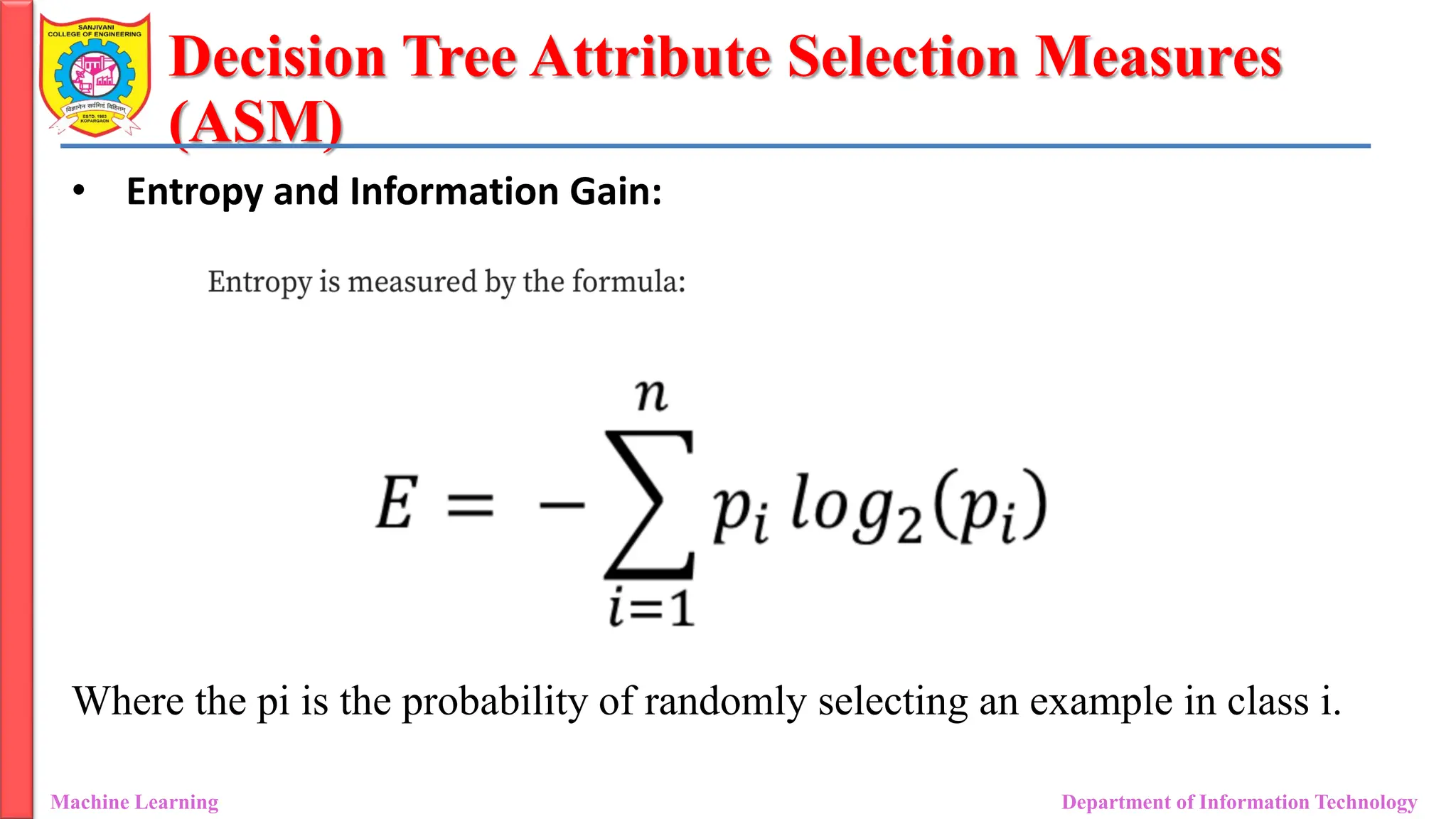
Where the pi is the probability of randomly selecting an example in class i.
23.
Decision Tree AttributeSelection Measures
(ASM)
Machine Learning Department of Information Technology
• Entropy and Information Gain:
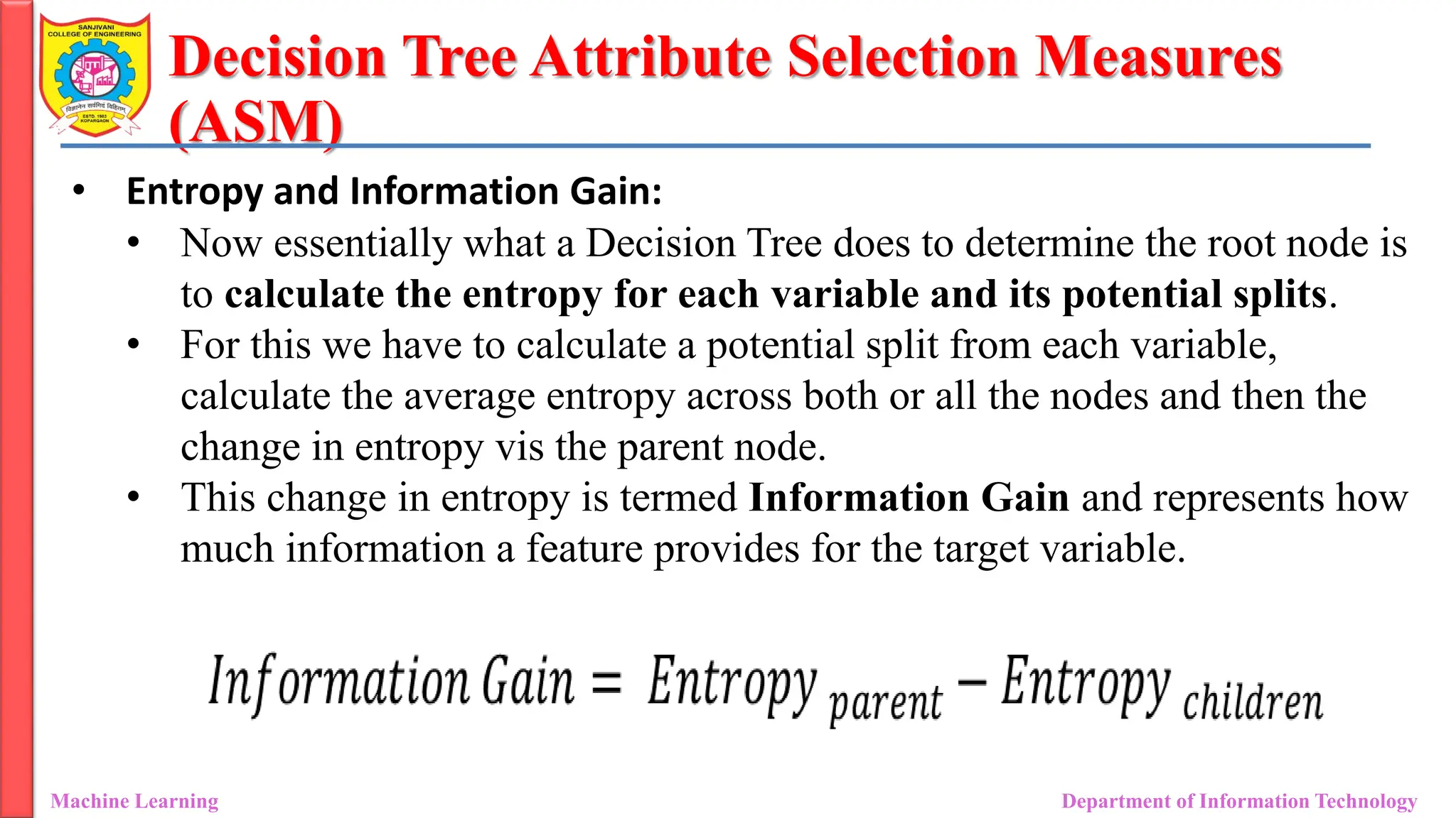
• Now essentially what a Decision Tree does to determine the root node is
to calculate the entropy for each variable and its potential splits.
• For this we have to calculate a potential split from each variable,
calculate the average entropy across both or all the nodes and then the
change in entropy vis the parent node.
• This change in entropy is termed Information Gain and represents how
much information a feature provides for the target variable.
24.
Decision Tree AttributeSelection Measures
(ASM)
Machine Learning Department of Information Technology
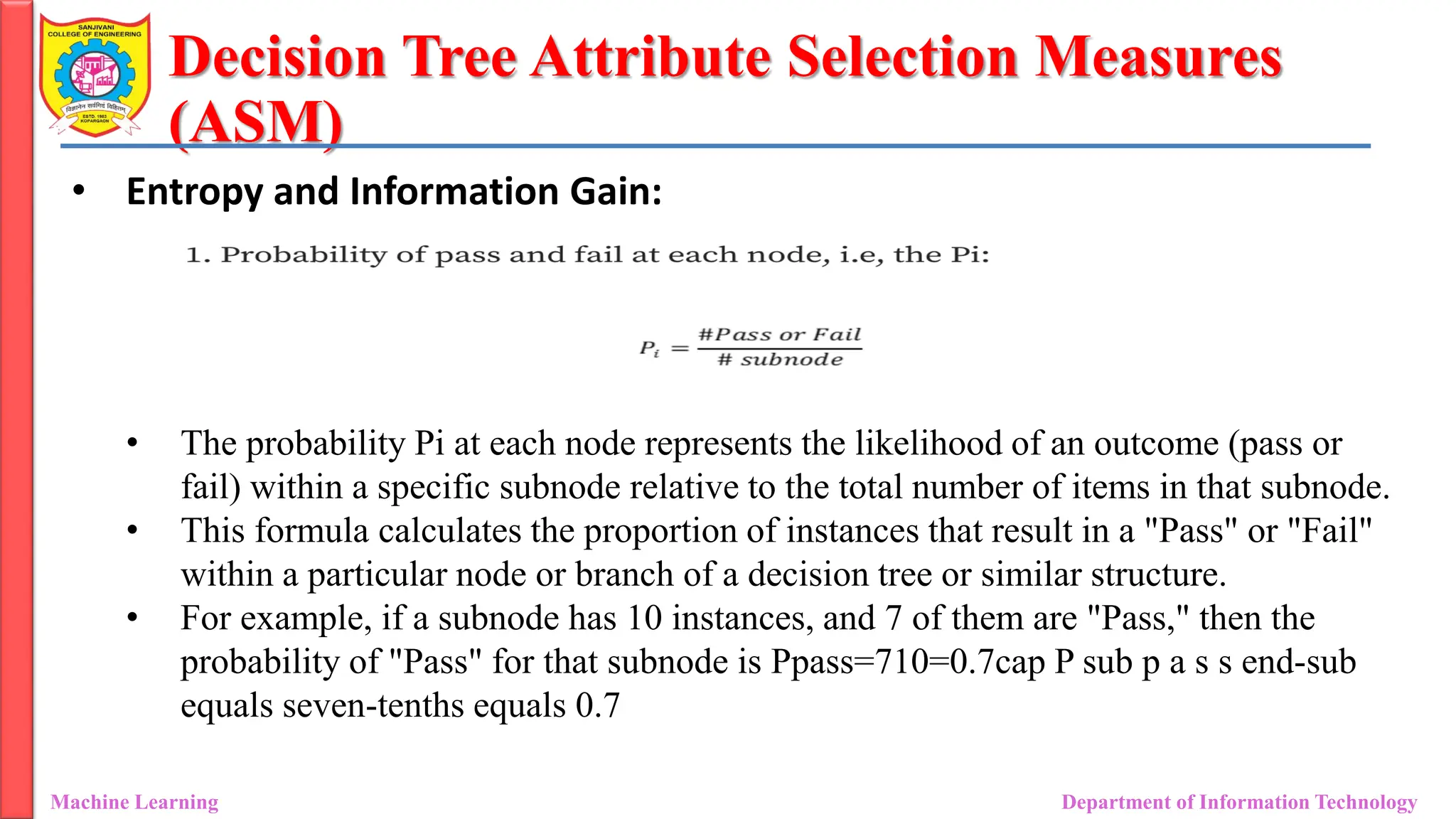
• Entropy and Information Gain:
• The probability Pi at each node represents the likelihood of an outcome (pass or
fail) within a specific subnode relative to the total number of items in that subnode.
• This formula calculates the proportion of instances that result in a "Pass" or "Fail"
within a particular node or branch of a decision tree or similar structure.
• For example, if a subnode has 10 instances, and 7 of them are "Pass," then the
probability of "Pass" for that subnode is Ppass=710=0.7cap P sub p a s s end-sub
equals seven-tenths equals 0.7
25.
Decision Tree AttributeSelection Measures
(ASM)
Machine Learning Department of Information Technology
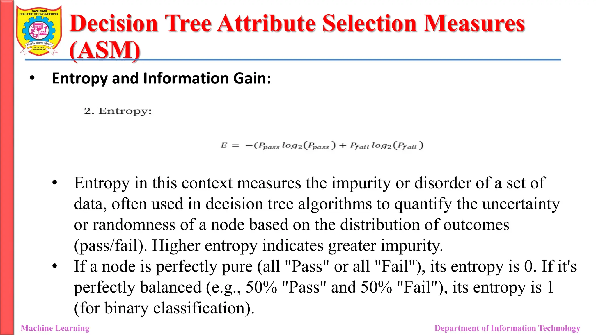
• Entropy and Information Gain:
• Entropy in this context measures the impurity or disorder of a set of
data, often used in decision tree algorithms to quantify the uncertainty
or randomness of a node based on the distribution of outcomes
(pass/fail). Higher entropy indicates greater impurity.
• If a node is perfectly pure (all "Pass" or all "Fail"), its entropy is 0. If it's
perfectly balanced (e.g., 50% "Pass" and 50% "Fail"), its entropy is 1
(for binary classification).
26.
Decision Tree AttributeSelection Measures
(ASM)
Machine Learning Department of Information Technology
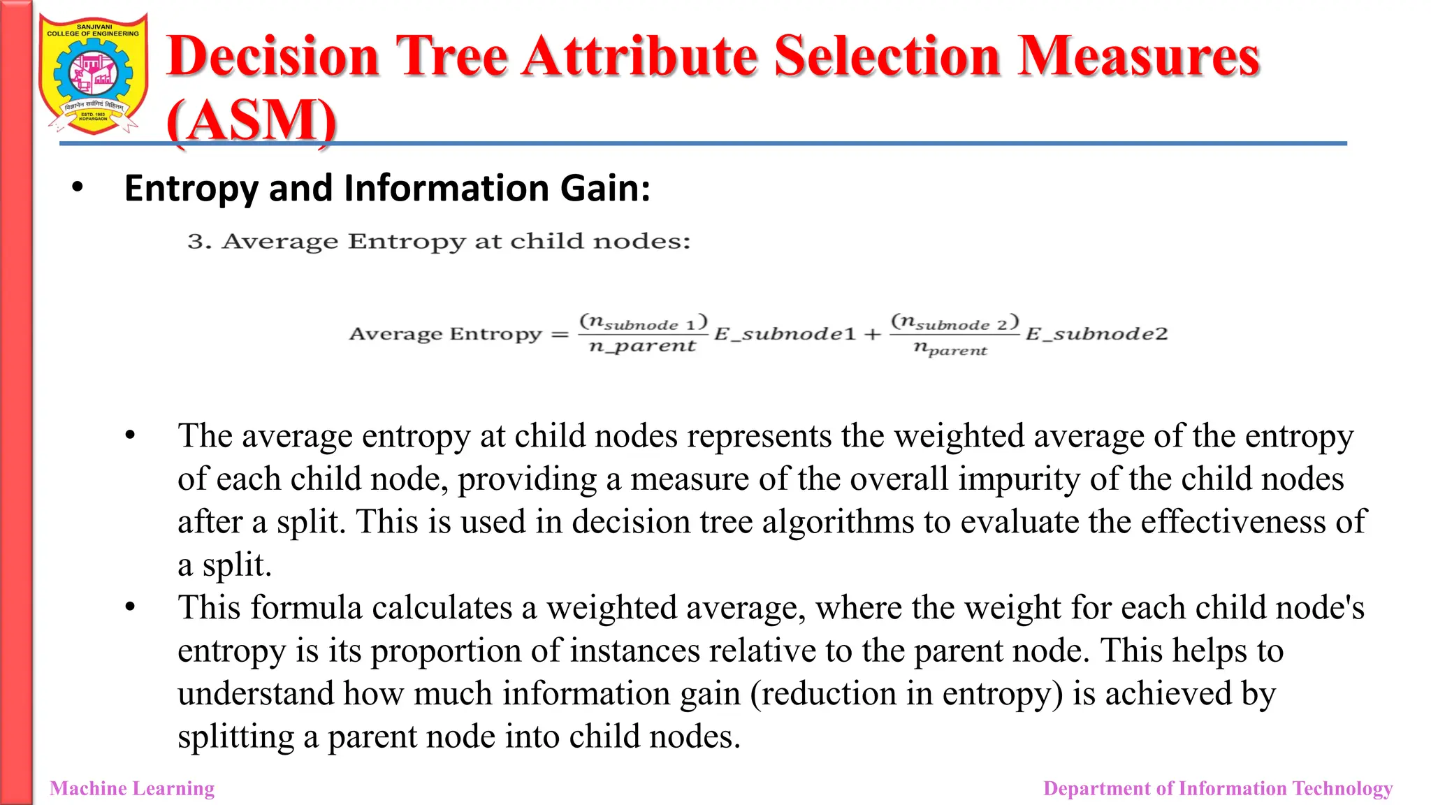
• Entropy and Information Gain:
• The average entropy at child nodes represents the weighted average of the entropy
of each child node, providing a measure of the overall impurity of the child nodes
after a split. This is used in decision tree algorithms to evaluate the effectiveness of
a split.
• This formula calculates a weighted average, where the weight for each child node's
entropy is its proportion of instances relative to the parent node. This helps to
understand how much information gain (reduction in entropy) is achieved by
splitting a parent node into child nodes.
27.
Decision Tree AttributeSelection Measures
(ASM)
Machine Learning Department of Information Technology
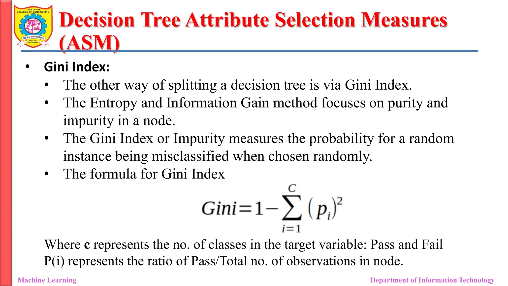
• Gini Index:
• The other way of splitting a decision tree is via Gini Index.
• The Entropy and Information Gain method focuses on purity and
impurity in a node.
• The Gini Index or Impurity measures the probability for a random
instance being misclassified when chosen randomly.
• The formula for Gini Index
Where c represents the no. of classes in the target variable: Pass and Fail
P(i) represents the ratio of Pass/Total no. of observations in node.
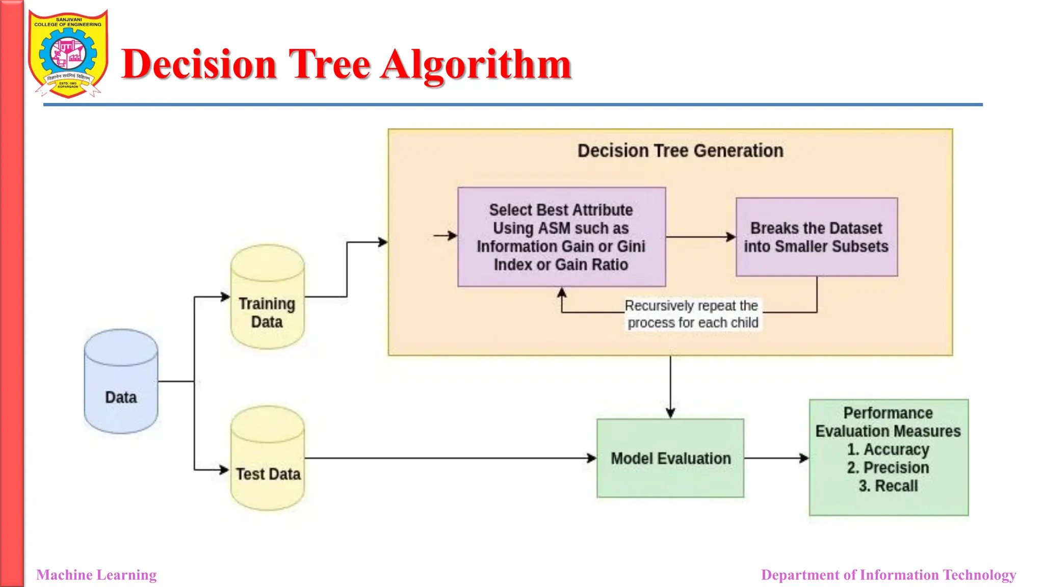
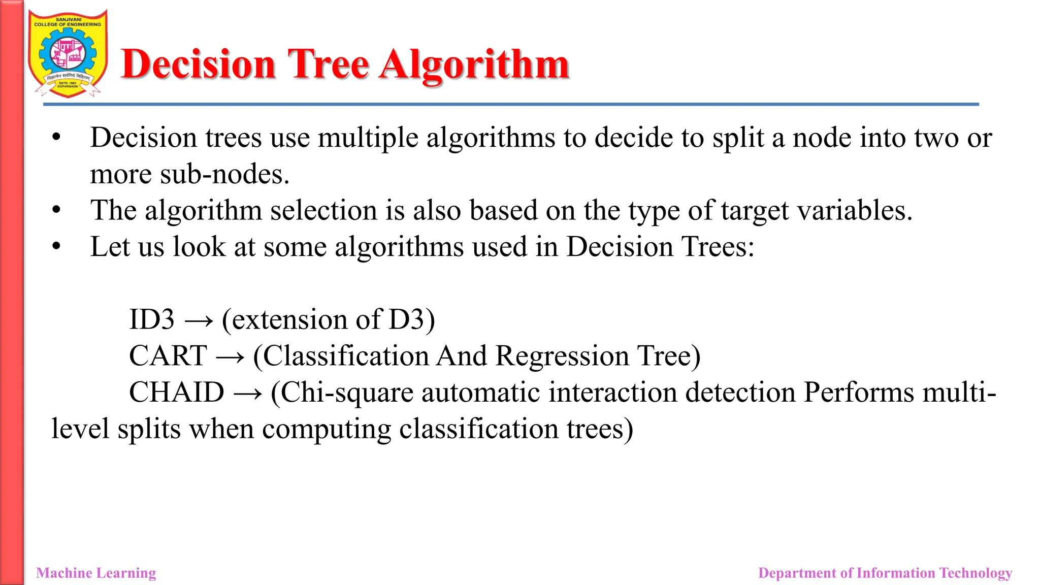
Decision Tree Algorithm
MachineLearning Department of Information Technology
• Decision trees use multiple algorithms to decide to split a node into two or
more sub-nodes.
• The algorithm selection is also based on the type of target variables.
• Let us look at some algorithms used in Decision Trees:
ID3 → (extension of D3)
CART → (Classification And Regression Tree)
CHAID → (Chi-square automatic interaction detection Performs multi-
level splits when computing classification trees)
30.
Decision Tree Algorithm
MachineLearning Department of Information Technology
• When to Stop Splitting?
• We can set the maximum depth of our decision tree using the
max_depth parameter.
• The more the value of max_depth, the more complex your tree will
• Another way is to set the minimum number of samples for each spilt.
• It is denoted by min_samples_split.
• Here we specify the minimum number of samples required to do a spilt.
31.
Decision Tree Algorithm
MachineLearning Department of Information Technology
• Pruning:
• Pruning is a method that can help us avoid overfitting.
• It helps in improving the performance of the Decision tree by cutting
the nodes or sub-nodes which are not significant.
• Additionally, it removes the branches which have very low importance.
• There are mainly 2 ways for pruning:
• Pre-pruning
• Post-pruning
32.
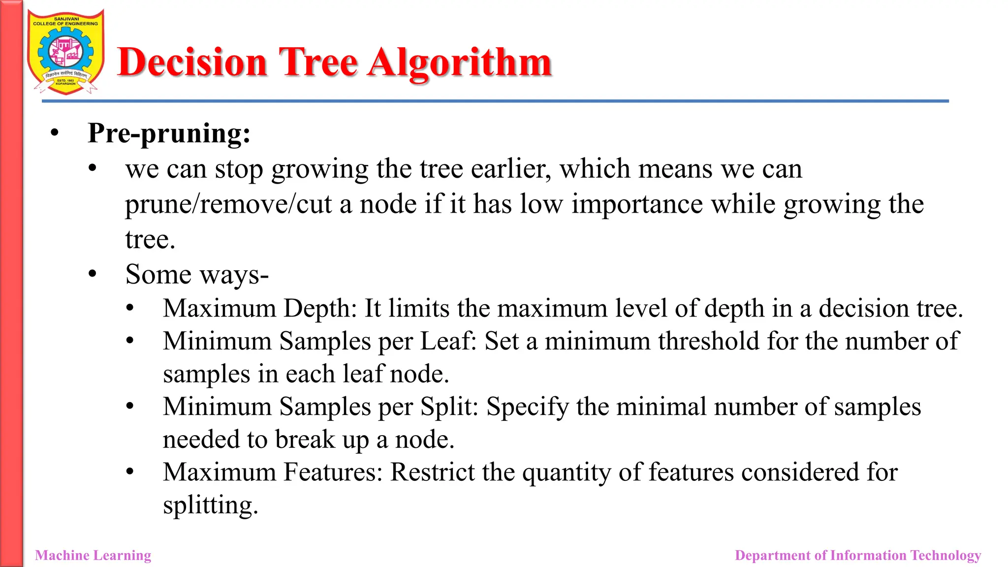
Decision Tree Algorithm
MachineLearning Department of Information Technology
• Pre-pruning:
• we can stop growing the tree earlier, which means we can
prune/remove/cut a node if it has low importance while growing the
tree.
• Some ways-
• Maximum Depth: It limits the maximum level of depth in a decision tree.
• Minimum Samples per Leaf: Set a minimum threshold for the number of
samples in each leaf node.
• Minimum Samples per Split: Specify the minimal number of samples
needed to break up a node.
• Maximum Features: Restrict the quantity of features considered for
splitting.
33.
Decision Tree Algorithm
MachineLearning Department of Information Technology
• Post-pruning (Reduce Nodes):
• Once our tree is built to its depth, we can start pruning the nodes based
on their significance.
• We can remove branches or nodes to improve the model's ability to
generalize.
• Cost-Complexity Pruning (CCP): This method assigns a price to each subtree
primarily based on its accuracy and complexity, then selects the subtree with the
lowest fee.
• Reduced Error Pruning: Removes branches that do not significantly affect the
overall accuracy.
• Minimum Impurity Decrease: Prunes nodes if the decrease in impurity (Gini
impurity or entropy) is beneath a certain threshold.
• Minimum Leaf Size: Removes leaf nodes with fewer samples than a specified
threshold.
34.
Decision Tree Algorithm
MachineLearning Department of Information Technology
# Load libraries
import pandas as pd
from sklearn.tree import DecisionTreeClassifier
from sklearn.model_selection import train_test_split
from sklearn import metrics
col_names = ['pregnant', 'glucose', 'bp', 'skin', 'insulin', 'bmi', 'pedigree', 'age',
'label']
# load dataset
pima = pd.read_csv("diabetes.csv", names=col_names)
X_train, X_test, y_train, y_test = train_test_split(X, y, test_size=0.3,
random_state=1)
35.
Decision Tree Algorithm
MachineLearning Department of Information Technology
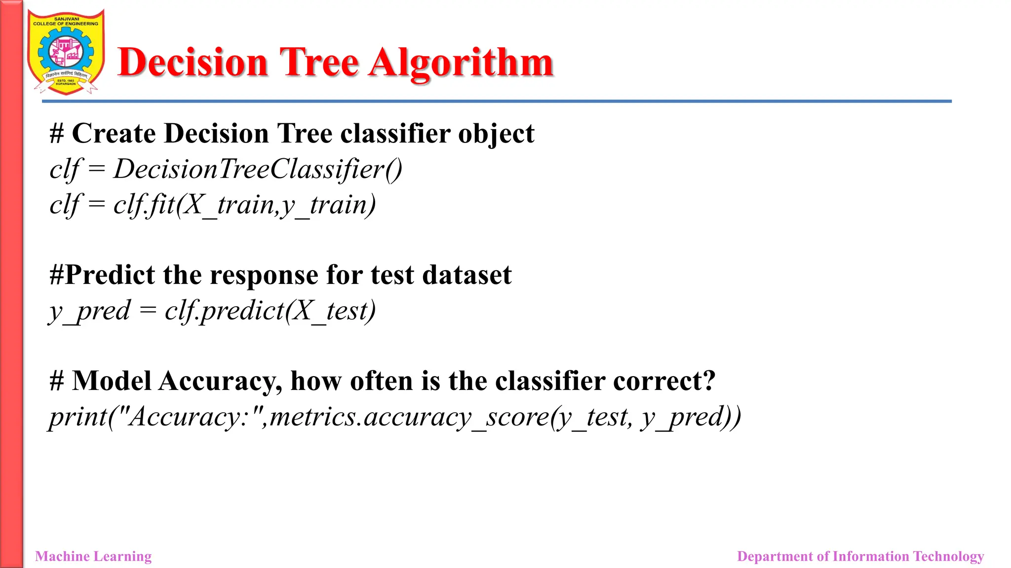
# Create Decision Tree classifier object
clf = DecisionTreeClassifier()
clf = clf.fit(X_train,y_train)
#Predict the response for test dataset
y_pred = clf.predict(X_test)
# Model Accuracy, how often is the classifier correct?
print("Accuracy:",metrics.accuracy_score(y_test, y_pred))

![Decision Tree Algorithm
Machine Learning Department of Information Technology
# Load libraries
import pandas as pd
from sklearn.tree import DecisionTreeClassifier
from sklearn.model_selection import train_test_split
from sklearn import metrics
col_names = ['pregnant', 'glucose', 'bp', 'skin', 'insulin', 'bmi', 'pedigree', 'age',
'label']
# load dataset
pima = pd.read_csv("diabetes.csv", names=col_names)
X_train, X_test, y_train, y_test = train_test_split(X, y, test_size=0.3,
random_state=1)](https://image.slidesharecdn.com/unit3classificationdecisiontree-250825105807-d3685cbf/75/Unit-3_Classification_Decision-Tree_ASM-pdf-34-2048.jpg)