Supervised learning Algorithms: Decision Trees, Tree pruning, Rule-base Classification, Naïve Bayes, Bayesian Network. Support Vector Machines, k-Nearest Neighbor, Ensemble Learning and Random Forest algorithm

1. BCA 313
Machine Learning with Python
Unit-2

2. SYLLABUS
Supervised learning Algorithms:
Decision Trees, Tree pruning, Rule-base
Classification, Naïve Bayes, Bayesian
Network. Support Vector Machines, k-
Nearest Neighbor, Ensemble Learning
and Random Forest algorithm

3. Decision Trees
 Decision Tree is a Supervised learning technique that can be used for both classification
and Regression problems, but mostly it is preferred for solving Classification problems.
 It is a tree-structured classifier, where internal nodes represent the features of a dataset,
branches represent the decision rules and each leaf node represents the outcome.
 The goal is to create a model that predicts the value of a target variable by learning
simple decision rules inferred from the data features.
 Decision trees can be constructed by an algorithmic approach that can split the dataset in
different ways based on different conditions.
 The decisions or the test are performed on the basis of features of the given dataset.
 It is a graphical representation for getting all the possible solutions to a problem/decision
based on given conditions.
 Though the decision tree can handle both categorical and numerical values but sklearn
requires the data to be numerical. So, the categorical data must be converted to
numerical.
 There are a few known algorithms in DTs such as ID3, C4.5, CART, C5.0, CHAID, QUEST,
CRUISE.

4. Terminology
 Root Node: Root node is from where the decision
tree starts. It represents the entire dataset, which
further gets divided into two or more homogeneous
sets.
 Leaf Node: Leaf nodes are the final output node, and
the tree cannot be segregated further after getting a
leaf node.
 Splitting: Splitting is the process of dividing the
decision node/root node into sub-nodes according to
the given conditions.
 Branch/Sub Tree: A tree formed by splitting the tree.
 Pruning: Pruning is the process of removing the
unwanted branches from the tree.
 Parent/Child node: The root node of the tree is
called the parent node, and other nodes are called
the child nodes.

5. Decision tree Algorithm
• Step-1: Begin the tree with the root node, says S,
which contains the complete dataset.
• Step-2: Find the best attribute in the dataset
using Attribute Selection Measure (ASM) like
Gini index or Information Gain
• Step-3: Divide the S into subsets that contains
possible values for the best attributes.
• Step-4: Generate the decision tree node, which
contains the best attribute.
• Step-5: Recursively make new decision trees
using the subsets of the dataset created in step -
3. Continue this process until a stage is reached
where you cannot further classify the nodes and
called the final node as a leaf node.

6. Attribute Selection Measures
 While implementing a Decision tree, the main issue arises that how to select the best attribute for the root node and for sub-nodes. So,
to solve such problems there is a technique which is called as Attribute selection measure or ASM. By this measurement, we can easily
select the best attribute for the nodes of the tree. There are two popular techniques for ASM, which are:
 1. Information Gain:
 Information gain is the measurement of changes in entropy after the segmentation of a dataset based on an attribute.
 It calculates how much information a feature provides us about a class.
 According to the value of information gain, we split the node and build the decision tree.
 A decision tree algorithm always tries to maximize the value of information gain, and a node/attribute having the highest information
gain is split first. It can be calculated using the below formula:
 Information Gain= Entropy(S)- [(Weighted Avg) *Entropy(each feature)
 Entropy: Entropy is a metric to measure the impurity in a given attribute. It specifies randomness in data. Entropy can be calculated as:
 Entropy(s)= -P(yes)log2 P(yes)- P(no) log2 P(no)
 Where,
 S= Total number of samples
 P(yes)= probability of yes
 P(no)= probability of no
 2. Gini Index:
 Gini index is a measure of impurity or purity used while creating a decision tree in the CART(Classification and Regression Tree)
algorithm.
 An attribute with the low Gini index should be preferred as compared to the high Gini index.
 It only creates binary splits, and the CART algorithm uses the Gini index to create binary splits.
 Gini index can be calculated using the below formula:
 Gini Index= 1- ∑jPj2
 For more information : Machine Learning from Scratch: Decision Trees - KDnuggets

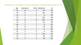
7. Decision tree to decide if a person should go to watch comedy show or not
Age Experience Rank Nationality Go
36 10 9 UK NO
42 12 4 USA NO
23 4 6 N NO
52 4 4 USA NO
43 21 8 USA YES
44 14 5 UK NO
66 3 7 N YES
35 14 9 UK YES
52 13 7 N YES
35 5 9 N YES
24 3 5 USA NO
18 3 7 UK YES
45 9 9 UK YES

8.  import pandas as pd
 from sklearn import tree
 from sklearn import metrics
 import matplotlib.pyplot as plt

df=pd.read_csv("decision tree comedy.csv")
 print(df.head())
 print(df.info())
 #We have to convert the non numerical columns 'Nationality' and 'Go' into numerical
values.
 #Pandas has a map() method that takes a dictionary with information on how to convert
the values.
 d = {'UK': 0, 'USA': 1, 'N': 2}
 df['Nationality'] = df['Nationality'].map(d)
 d = {'YES': 1, 'NO': 0}
 df['Go'] = df['Go'].map(d)
 print(df)
 # Split data in feature and target variables
 X=df.drop('Go',axis=1)
 y=df['Go']
 clf=tree.DecisionTreeClassifier()
 //we can pass argument (criterion=‘entropy’) to use instead of gini index
 clf.fit(X.values,y)
 tree.plot_tree(clf,feature_names=['Age', 'Experience', 'Rank', 'Nationality'])
 print(clf.predict([[40, 10, 7, 1]]))

10. True - 5 Comedians End Here:
gini = 0.0 means all of the samples got the
same result.
samples = 5 means that there are 5
comedians left in this branch.
value = [5, 0] means that 5 will get a "NO"
and 0 will get a "GO".
True - 4 Comedians Continue:
Age <= 35.5 means that comedians at the age of
35.5 or younger will follow the arrow to the left,
and the rest will follow the arrow to the right.
gini = 0.375 means that about 37,5% of the samples
would go in one direction.
samples = 4 means that there are 4 comedians left
in this branch (4 comedians from the UK).
value = [1, 3] means that of these 4 comedians, 1
will get a "NO" and 3 will get a "GO".

11. Rank <= 6.5 means that every comedian with a rank of 6.5 or lower will follow
the True arrow (to the left), and the rest will follow the False arrow (to the
right).
gini = 0.497 refers to the quality of the split, and is always a number between
0.0 and 0.5, where 0.0 would mean all of the samples got the same result, and
0.5 would mean that the split is done exactly in the middle.
Gini = 1 - (x/n)2 - (y/n)2
Where x is the number of positive answers("GO"), n is the number of samples,
and y is the number of negative answers ("NO"), which gives us this calculation:
1 - (7 / 13)2 - (6 / 13)2 = 0.497
samples = 13 means that there are 13 comedians left at this point in the
decision, which is all of them since this is the first step.
value = [6, 7] means that of these 13 comedians, 6 will get a "NO", and 7 will get
a "GO".
Note : All nodes with gini = 0.0 are leaf nodes

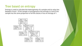
12. Tree based on entropy
Entropy is used to calculate the heterogeneity of a sample and its value lies
between 0 and 1. If the sample is homogeneous the entropy is 0 and if the
sample has the same proportion of all the classes it has an entropy of 1.

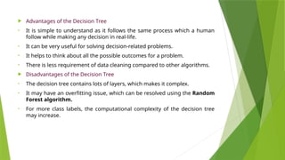
13.  Advantages of the Decision Tree
• It is simple to understand as it follows the same process which a human
follow while making any decision in real-life.
• It can be very useful for solving decision-related problems.
• It helps to think about all the possible outcomes for a problem.
• There is less requirement of data cleaning compared to other algorithms.
 Disadvantages of the Decision Tree
• The decision tree contains lots of layers, which makes it complex.
• It may have an overfitting issue, which can be resolved using the Random
Forest algorithm.
• For more class labels, the computational complexity of the decision tree
may increase.

14. Tree Pruning
 Pruning is a data compression technique in machine learning and search algorithms that reduces the
size of decision trees by removing sections of the tree that are non-critical and redundant to classify
instances.
 Pruning reduces the complexity of the final classifier, and hence improves predictive accuracy by the
reduction of overfitting.
 One of the questions that arises in a decision tree algorithm is the optimal size of the final tree. A
tree that is too large risks overfitting the training data and poorly generalizing to new samples. A
small tree might not capture important structural information about the sample space. However, it is
hard to tell when a tree algorithm should stop because it is impossible to tell if the addition of a
single extra node will dramatically decrease error.
 Pruning processes can be divided into two types (pre- and post-pruning).
 Pre-pruning procedures prevent a complete induction of the training set by replacing a stop () criterion
in the induction algorithm (e.g. max. Tree depth or information gain (Attr)> minGain). Pre-pruning
methods are considered to be more efficient because they do not induce an entire set, but rather trees
remain small from the start. Prepruning methods share a common problem, the horizon effect. This is to
be understood as the undesired premature termination of the induction by the stop () criterion.
 Post-pruning (or just pruning) is the most common way of simplifying trees. Here, nodes and subtrees
are replaced with leaves to reduce complexity. Pruning can not only significantly reduce the size but
also improve the classification accuracy of unseen objects. It may be the case that the accuracy of the
assignment on the train set deteriorates, but the accuracy of the classification properties of the tree
increases overall.

15. Practice Question
 Load the iris dataset. Create a decision tree and analyse the tree.

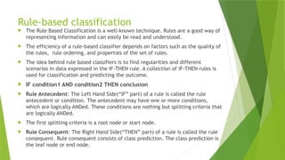
16. Rule-based classification
 The Rule Based Classification is a well-known technique. Rules are a good way of
representing information and can easily be read and understood.
 The efficiency of a rule-based classifier depends on factors such as the quality of
the rules, rule ordering, and properties of the set of rules.
 The idea behind rule based classifiers is to find regularities and different
scenarios in data expressed in the IF-THEN rule. A collection of IF-THEN rules is
used for classification and predicting the outcome.
 IF condition1 AND condition2 THEN conclusion
 Rule Antecedent: The Left Hand Side(“IF” part) of a rule is called the rule
antecedent or condition. The antecedent may have one or more conditions,
which are logically ANDed. These conditions are nothing but splitting criteria that
are logically ANDed.
 The first splitting criteria is a root node or start node.
 Rule Consequent: The Right Hand Side(“THEN” part) of a rule is called the rule
consequent. Rule consequent consists of class prediction. The class prediction is
the leaf node or end node.

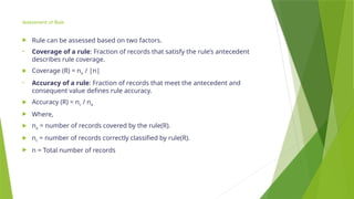
17. Assessment of Rule
 Rule can be assessed based on two factors.
• Coverage of a rule: Fraction of records that satisfy the rule’s antecedent
describes rule coverage.
 Coverage (R) = na / |n|
• Accuracy of a rule: Fraction of records that meet the antecedent and
consequent value defines rule accuracy.
 Accuracy (R) = nc / na
 Where,
 na = number of records covered by the rule(R).
 nc = number of records correctly classified by rule(R).
 n = Total number of records

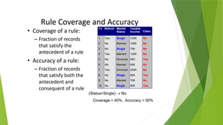
18.  Characteristics of Rule based Classifiers
 1) Rules may not be mutually exclusive. Different rules are generated for data,
so it is possible that many rules can cover the same record.
 2) Rules may not be exhaustive. It is possible that some of the data entries
may not be covered by any of the rules.
 Advantages of Rule Based Data Mining Classifiers
• Highly expressive.
• Easy to interpret.
• Easy to generate.
• Capability to classify new records rapidly.
• Performance is comparable to other classifiers.

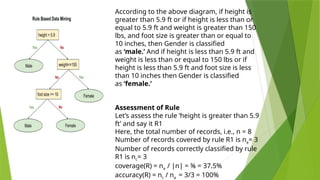
19. According to the above diagram, if height is
greater than 5.9 ft or if height is less than or
equal to 5.9 ft and weight is greater than 150
lbs, and foot size is greater than or equal to
10 inches, then Gender is classified
as ‘male.’ And if height is less than 5.9 ft and
weight is less than or equal to 150 lbs or if
height is less than 5.9 ft and foot size is less
than 10 inches then Gender is classified
as ‘female.’
Assessment of Rule
Let’s assess the rule ‘height is greater than 5.9
ft’ and say it R1
Here, the total number of records, i.e., n = 8
Number of records covered by rule R1 is na= 3
Number of records correctly classified by rule
R1 is nc= 3
coverage(R) = na / |n| = ⅜ = 37.5%
accuracy(R) = nc / na = 3/3 = 100%

21. Naïve Bayes
 Naïve Bayes algorithm is a supervised learning algorithm, which is based on Bayes
theorem and used for solving classification problems.
 It is mainly used in text classification that includes a high-dimensional training
dataset.
 Naïve Bayes Classifier is one of the simple and most effective Classification algorithms
which helps in building the fast machine learning models that can make quick
predictions.
 It is a probabilistic classifier, which means it predicts on the basis of the probability of
an object.
 Naive Bayes is known for its simplicity, efficiency, and effectiveness in handling
high-dimensional data.
 Some popular examples of Naïve Bayes Algorithm are spam filtration, Sentimental
analysis, and classifying articles.
 Naive Bayes is a classification algorithm for binary (two-class) and multiclass
classification problems.
 It is efficient when the dataset is relatively small and the features are conditionally
independent.

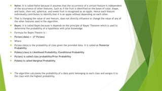
22.  Naïve: It is called Naïve because it assumes that the occurrence of a certain feature is independent
of the occurrence of other features. Such as if the fruit is identified on the bases of color, shape,
and taste, then red, spherical, and sweet fruit is recognized as an apple. Hence each feature
individually contributes to identify that it is an apple without depending on each other.
 That is changing the value of one feature, does not directly influence or change the value of any of
the other features used in the algorithm.
 Bayes: It is called Bayes because it depends on the principle of Bayes' Theorem which is used to
determine the probability of a hypothesis with prior knowledge.
 Formula for Bayes Theorm is :
 P(class|data) = ()* P(class)
 Where
 P(class|data) is the probability of class given the provided data. It is called as Posterior
Probability
 P(data|class) is Likelihood Probability /Conditional Probability
 P(class) is called class probability/Prior Probability
 P(data) is called Marginal Probability
 The algorithm calculates the probability of a data point belonging to each class and assigns it to
the class with the highest probability.

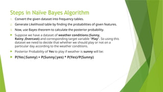
23. Steps in Naïve Bayes Algorithm
1. Convert the given dataset into frequency tables.
2. Generate Likelihood table by finding the probabilities of given features.
3. Now, use Bayes theorem to calculate the posterior probability.
 Suppose we have a dataset of weather conditions (Sunny,
Rainy ,Overcast) and corresponding target variable "Play". So using this
dataset we need to decide that whether we should play or not on a
particular day according to the weather conditions.
 Posterior Probability of Yes to play if weather is sunny will be:
 P(Yes|Sunny) = P(Sunny|yes) * P(Yes)/P(Sunny)

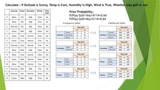
24. Outlook Temp Humidity Windy Play
Golf
0 Rainy Hot High False No
1 Rainy Hot High True No
2 Overcast Hot High False Yes
3 Sunny Mild High False Yes
4 Sunny Cool Normal False Yes
5 Sunny Cool Normal True No
6 Overcast Cool Normal True Yes
7 Rainy Mild High False No
8 Rainy Cool Normal False Yes
9 Sunny Mild Normal False Yes
10 Rainy Mild Normal True Yes
11 Overcast Mild High True Yes
12 Overcast Hot Normal False Yes
13 Sunny Mild High True No
Prior Probability:
P(Play Golf=Yes)=9/14=0.64
P(Play Golf=No)=5/14=0.64
Calculate : If Outlook is Sunny, Temp is Cool, Humidity is High, Wind is True, Whether play golf or not

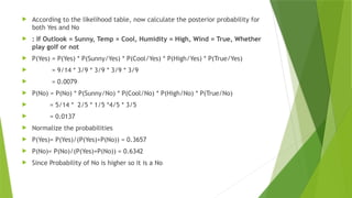
25.  According to the likelihood table, now calculate the posterior probability for
both Yes and No
 : If Outlook = Sunny, Temp = Cool, Humidity = High, Wind = True, Whether
play golf or not
 P(Yes) = P(Yes) * P(Sunny/Yes) * P(Cool/Yes) * P(High/Yes) * P(True/Yes)
 = 9/14 * 3/9 * 3/9 * 3/9 * 3/9
 = 0.0079
 P(No) = P(No) * P(Sunny/No) * P(Cool/No) * P(High/No) * P(True/No)
 = 5/14 * 2/5 * 1/5 *4/5 * 3/5
 = 0.0137
 Normalize the probabilities
 P(Yes)= P(Yes)/(P(Yes)+P(No)) = 0.3657
 P(No)= P(No)/(P(Yes)+P(No)) = 0.6342
 Since Probability of No is higher so it is a No

26. Practice Question
If there is a nuclear family,
with young people having
medium income status,
predict whether they can
buy a car or not

27. Types of Naïve Bayes
 Gaussian Naive Bayes
 This type of Naive Bayes is used when variables are continuous in nature. It assumes that all
the variables have a normal distribution. So if you have some variables which do not have this
property, you might want to transform them to the features having distribution normal.
 Multinomial Naive Bayes
 This is used when the features represent the frequency. Suppose you have a text document and
you extract all the unique words and create multiple features where each feature represents
the count of the word in the document. In such a case, we have a frequency as a feature. In
such a scenario, we use multinomial Naive Bayes. It ignores the non-occurrence of the
features. So, if you have frequency 0 then the probability of occurrence of that feature will be
0 hence multinomial naive Bayes ignores that feature. It is known to work well with text
classification problems.
 Bernoulli Naive Bayes
 This is used when features are binary. So, instead of using the frequency of the word, if you
have discrete features in 1s and 0s that represent the presence or absence of a feature. In that
case, the features will be binary and we will use Bernoulli Naive Bayes.
 Also, this method will penalize the non-occurrence of a feature, unlike multinomial Naive
Bayes.

28.  from sklearn.naive_bayes import GaussianNB
 import pandas as pd
 from sklearn.model_selection import train_test_split
 from sklearn import metrics
 import matplotlib.pyplot as plt

df=pd.read_csv("iris_dataset.csv")
 print(df.head())
 print(df.info())
# Split data in feature and target variables
 X=df.drop('target',axis=1)
 y=df['target']
 print(y.value_counts()) #check the label distribution
 # spliiting data into training and test data
 X_train, X_test, y_train, y_test = train_test_split(X, y, test_size=0.25, random_state=16)
 print(y_test.value_counts()) #check the label distribution in test class
 nb=GaussianNB() # if we do not write max_iter it gives warning. So as size of data increases we inc number
 nb.fit(X_train.values,y_train) #train the mode
 predicted=nb.predict(X_test.values) #predict and store the predicted values
 cm=metrics.confusion_matrix(y_test,predicted) #generate a confusion matrix
 print(cm)
 cm_display = metrics.ConfusionMatrixDisplay(confusion_matrix = cm, display_labels = ['Iris-setosa','Iris-
versicolor','Iris-virginica' ]) #plot confusion matrix
print(metrics.accuracy_score(y_test,predicted)) #print the accuracy
 print(metrics.classification_report(y_test,predicted)) #generate classification report
cm_display.plot()
 plt.show()

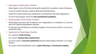
30.  Advantages of Naïve Bayes Classifier:
• Naïve Bayes is one of the fast and easy ML algorithms to predict a class of datasets.
• It can be used for Binary as well as Multi-class Classifications.
• It performs well in Multi-class predictions as compared to the other Algorithms.
• It is the most popular choice for text classification problems.
 Disadvantages of Naïve Bayes Classifier:
• Naive Bayes assumes that all features are independent or unrelated, so it cannot
learn the relationship between features.
• It assumes that all features contribute equally to the outcome which is not true in
real world cases.
 Applications of Naïve Bayes Classifier:
• It is used for Credit Scoring.
• It is used in medical data classification.
• It can be used in real-time predictions because Naïve Bayes Classifier is an eager
learner.
• It is used in Text classification such as Spam filtering and Sentiment analysis.

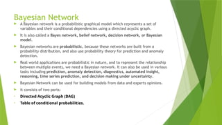
31. Bayesian Network
 A Bayesian network is a probabilistic graphical model which represents a set of
variables and their conditional dependencies using a directed acyclic graph.
 It is also called a Bayes network, belief network, decision network, or Bayesian
model.
 Bayesian networks are probabilistic, because these networks are built from a
probability distribution, and also use probability theory for prediction and anomaly
detection.
 Real world applications are probabilistic in nature, and to represent the relationship
between multiple events, we need a Bayesian network. It can also be used in various
tasks including prediction, anomaly detection, diagnostics, automated insight,
reasoning, time series prediction, and decision making under uncertainty.
 Bayesian Network can be used for building models from data and experts opinions.
 it consists of two parts:
• Directed Acyclic Graph (DAG)
• Table of conditional probabilities.

32.  The generalized form of Bayesian network that represents and solve decision problems under uncertain
knowledge is known as an Influence diagram.
 A Bayesian network graph is made up of nodes and Arcs (directed links),
• Each node corresponds to the random variables, and a variable can be continuous or discrete.
• Arc or directed arrows represent the causal relationship or conditional probabilities between random
variables. These directed links or arrows connect the pair of nodes in the graph. These links represent that
one node directly influence the other node
 The Bayesian network has mainly two components:
• Causal Component
• Actual numbers
 Each node in the Bayesian network has condition probability distribution P(Xi |Parent(Xi) ), which
determines the effect of the parent on that node.
• Bayesian network is based on Joint probability distribution and conditional probability.
• Joint probability distribution:
• If we have variables x1, x2, x3,....., xn, then the probabilities of a different combination of x1, x2, x3.. xn,
are known as Joint probability distribution.
• P[x1, x2, x3,....., xn], it can be written as the following way in terms of the joint probability distribution.
• = P[x1| x2, x3,....., xn]P[x2, x3,....., xn]
• = P[x1| x2, x3,....., xn]P[x2|x3,....., xn]....P[xn-1|xn]P[xn].
• In general for each variable Xi, we can write the equation as:
• P(Xi|Xi-1,........., X1) = P(Xi |Parents(Xi ))

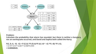
33. Problem:
Calculate the probability that alarm has sounded, but there is neither a burglary,
nor an earthquake occurred, and David and Sophia both called the Harry.
P(S, D, A, ¬B, ¬E) = P (S|A) *P (D|A)*P (A|¬B ^ ¬E) *P (¬B) *P (¬E).
= 0.75* 0.91* 0.001* 0.998*0.999
= 0.00068045.
0.001

35. Support Vector Machine(SVM)
 Support Vector Machine or SVM is one of the most popular Supervised Learning
algorithms, which is used for Classification as well as Regression problems.
However, primarily, it is used for Classification problems in Machine Learning.
 The goal of the SVM algorithm is to create the best line or decision boundary
that can segregate n-dimensional space into classes so that we can easily put
the new data point in the correct category in the future. This best decision
boundary is called a hyperplane.
 SVM chooses the extreme points/vectors that help in creating the hyperplane.
These extreme cases are called as support vectors, and hence algorithm is
termed as Support Vector Machine.
 SVM algorithm can be used for Face detection, image classification, text
categorization, etc.

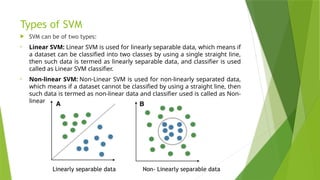
36. Types of SVM
 SVM can be of two types:
• Linear SVM: Linear SVM is used for linearly separable data, which means if
a dataset can be classified into two classes by using a single straight line,
then such data is termed as linearly separable data, and classifier is used
called as Linear SVM classifier.
• Non-linear SVM: Non-Linear SVM is used for non-linearly separated data,
which means if a dataset cannot be classified by using a straight line, then
such data is termed as non-linear data and classifier used is called as Non-
linear SVM classifier.
Linearly separable data Non- Linearly separable data

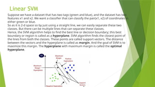
37. Linear SVM
Suppose we have a dataset that has two tags (green and blue), and the dataset has two
features x1 and x2. We want a classifier that can classify the pair(x1, x2) of coordinates in
either green or blue.
So as it is 2-d space so by just using a straight line, we can easily separate these two
classes. But there can be multiple lines that can separate these classes.
Hence, the SVM algorithm helps to find the best line or decision boundary; this best
boundary or region is called as a hyperplane. SVM algorithm finds the closest point of
the lines from both the classes. These points are called support vectors. The distance
between the vectors and the hyperplane is called as margin. And the goal of SVM is to
maximize this margin. The hyperplane with maximum margin is called the optimal
hyperplane.

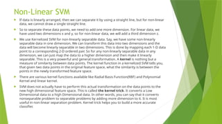
38. Non-Linear SVM
 If data is linearly arranged, then we can separate it by using a straight line, but for non-linear
data, we cannot draw a single straight line.
 So to separate these data points, we need to add one more dimension. For linear data, we
have used two dimensions x and y, so for non-linear data, we will add a third dimension z.
 We use Kernelized SVM for non-linearly separable data. Say, we have some non-linearly
separable data in one dimension. We can transform this data into two dimensions and the
data will become linearly separable in two dimensions. This is done by mapping each 1-D data
point to a corresponding 2-D ordered pair. So for any non-linearly separable data in any
dimension, we can just map the data to a higher dimension and then make it linearly
separable. This is a very powerful and general transformation. A kernel is nothing but a
measure of similarity between data points. The kernel function in a kernelized SVM tells you,
that given two data points in the original feature space, what the similarity is between the
points in the newly transformed feature space.
 There are various kernel functions available like Radial Basis Function(RBF) and Polynomial
Kernel and linear kernel.
 SVM does not actually have to perform this actual transformation on the data points to the
new high dimensional feature space. This is called the kernel trick. It converts a Low
Dimensional data to a high Dimensional data. In other words, you can say that it converts
nonseparable problem to separable problems by adding more dimension to it. It is most
useful in non-linear separation problem. Kernel trick helps you to build a more accurate
classifier.

39. Comparison of Linear and non-linear SVM

40.  Advantages of Support Vector Machine:
1. SVM works relatively well when there is a clear margin of separation between classes.
2. SVM is more effective in high dimensional spaces
3. VM works better when the data is Linear
4. With the help of the kernel trick, we can solve any complex problem
5. SVM is not sensitive to outliers
6. Can help us with Image classification
 Disadvantages of Support Vector Machine:
1. SVM algorithm is not suitable for large data sets.
2. SVM does not perform very well when the data set has more noise i.e. target classes are
overlapping.
3. In cases where the number of features for each data point exceeds the number of training
data samples, the SVM will underperform.
4. As the support vector classifier works by putting data points, above and below the
classifying hyperplane there is no probabilistic explanation for the classification.
5. For more info: https://www.datacamp.com/tutorial/svm-classification-scikit-learn-python

41.  from sklearn.svm import SVC
 import pandas as pd
 from sklearn.model_selection import train_test_split
 from sklearn import metrics
 import matplotlib.pyplot as plt

df=pd.read_csv("/content/drive/MyDrive/Colab Notebooks/ML BCA SEM 5/banknote-authentication.csv")
 print(df.head())
 print(df.info())
 # Split data in feature and target variables
 X=df.drop('class',axis=1)
 y=df['class']
 print(y.value_counts()) #check the label distribution
 # spliiting data into training and test data
 X_train, X_test, y_train, y_test = train_test_split(X, y, test_size=0.25, random_state=16)
 print(y_test.value_counts()) #check the label distribution in test class
 sv=SVC()
 #sv=SVC(kernel='linear')
 sv.fit(X_train.values,y_train) #train the mode
 predicted=sv.predict(X_test.values) #predict and store the predicted values
 cm=metrics.confusion_matrix(y_test,predicted) #generate a confusion matrix
 print(cm)
 cm_display = metrics.ConfusionMatrixDisplay(confusion_matrix = cm) #plot confusion matrix
 print(metrics.accuracy_score(y_test,predicted)) #print the accuracy
 print(metrics.classification_report(y_test,predicted)) #generate classification report
 cm_display.plot()
 plt.show()

43. KNN Algorithm
• K-Nearest Neighbour is one of the simplest Machine Learning algorithms based on
Supervised Learning technique.
• K-NN algorithm assumes the similarity between the new case/data and available
cases and put the new case into the category that is most similar to the available
categories.
• K-NN algorithm stores all the available data and classifies a new data point based
on the similarity. This means when new data appears then it can be easily classified
into a well suite category by using K- NN algorithm.
• K-NN algorithm can be used for Regression as well as for Classification but mostly it
is used for the Classification problems.
• K-NN is a non-parametric algorithm, which means it does not make any
assumption on underlying data.
• It is also called a lazy learner algorithm because it does not learn from the
training set immediately instead it stores the dataset and at the time of
classification, it performs an action on the dataset.
• KNN algorithm at the training phase just stores the dataset and when it gets new
data, then it classifies that data into a category that is much similar to the new data.

44. Working of KNN Algorithm
• Step-1: Select the number K of the neighbors
• Step-2: Calculate the Euclidean distance of K number of neighbors
• Step-3: Take the K nearest neighbors as per the calculated Euclidean
distance.
• Step-4: Among these k neighbors, count the number of the data points in
each category.
• Step-5: Assign the new data points to that category for which the number
of the neighbor is maximum i.e. Majority Voting

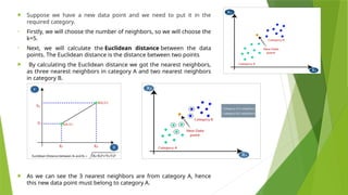
45.  Suppose we have a new data point and we need to put it in the
required category.
• Firstly, we will choose the number of neighbors, so we will choose the
k=5.
• Next, we will calculate the Euclidean distance between the data
points. The Euclidean distance is the distance between two points
 By calculating the Euclidean distance we got the nearest neighbors,
as three nearest neighbors in category A and two nearest neighbors
in category B.
 As we can see the 3 nearest neighbors are from category A, hence
this new data point must belong to category A.

46. Numerical Example
 https://people.revoledu.com/kardi/tutorial/KNN/KNN_Numerical-example.ht
ml
 https://www.freecodecamp.org/news/k-nearest-neighbors-algorithm-classifie
rs-and-model-example/

47.  from sklearn.neighbors import KNeighborsClassifier
 import pandas as pd
 from sklearn.model_selection import train_test_split
 from sklearn import metrics
 import matplotlib.pyplot as plt
df=pd.read_csv("/content/drive/MyDrive/Colab Notebooks/ML BCA SEM 5/iris_dataset.csv")
 #print(df.head())
 #print(df.info())
# Split data in feature and target variables
 X=df.drop('target',axis=1)
 y=df['target']
 print(y.value_counts()) #check the label distribution
 # spliiting data into training and test data
 X_train, X_test, y_train, y_test = train_test_split(X, y, test_size=0.25, random_state=16)
 print(y_test.value_counts()) #check the label distribution in test class
 clf=KNeighborsClassifier(n_neighbors=5) # default distance is calculated as minkowski
 clf.fit(X_train.values,y_train) #train the mode
 predicted=clf.predict(X_test.values) #predict and store the predicted values
 cm=metrics.confusion_matrix(y_test,predicted) #generate a confusion matrix
 print(cm)
 cm_display = metrics.ConfusionMatrixDisplay(confusion_matrix = cm, display_labels = ['Iris-
setosa','Iris-versicolor','Iris-virginica' ]) #plot confusion matrix
print(metrics.accuracy_score(y_test,predicted)) #print the accuracy
 print(metrics.classification_report(y_test,predicted)) #generate classification report
cm_display.plot()
 plt.show()

49. Ensemble Methods
 Ensemble methods is a machine learning technique that combines several
base models in order to produce one optimal predictive model.
 It enhances accuracy and resilience in forecasting by merging predictions
from multiple models.
 It aims to mitigate errors or biases that may exist in individual models by
leveraging the collective intelligence of the ensemble.
 The underlying concept behind ensemble learning is to combine the outputs
of diverse models to create a more precise prediction. By considering
multiple perspectives and utilizing the strengths of different models,
ensemble learning improves the overall performance of the learning system.
 Ensemble methods are ideal for regression and classification, where they
reduce bias and variance to boost the accuracy of models.

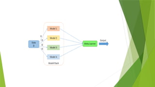
50. Types of Ensemble methods
 There are three main types of Ensembles:
 1. Bagging
 2. Boosting
 3. Stacking

51. Bagging
 Bagging, the short form for bootstrap aggregating, is mainly applied in classification
and regression. It increases the accuracy of models through decision trees, which
reduces variance to a large extent. The reduction of variance increases accuracy,
eliminating overfitting, which is a challenge to many predictive models.
 Bagging is classified into two types, i.e., bootstrapping and aggregation.
Bootstrapping is a sampling technique where samples are derived from the whole
population (set) using the replacement procedure. The sampling with replacement
method helps make the selection procedure randomized. The base learning
algorithm is run on the samples to complete the procedure.
 Aggregation in bagging is done to incorporate all possible outcomes of the
prediction and randomize the outcome. Without aggregation, predictions will not be
accurate because all outcomes are not put into consideration. Therefore, the
aggregation is based on the probability bootstrapping procedures or on the basis of
all outcomes of the predictive models.
 Bagging is advantageous since weak base learners are combined to form a single
strong learner that is more stable than single learners. It also eliminates any
variance, thereby reducing the overfitting of models. One limitation of bagging is
that it is computationally expensive. Thus, it can lead to more bias in models when
the proper procedure of bagging is ignored.

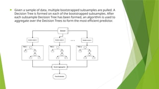
52.  Given a sample of data, multiple bootstrapped subsamples are pulled. A
Decision Tree is formed on each of the bootstrapped subsamples. After
each subsample Decision Tree has been formed, an algorithm is used to
aggregate over the Decision Trees to form the most efficient predictor.

53. Boosting
 Boosting is a sequential ensemble technique that learns from previous predictor
mistakes to make better predictions in the future. The technique combines several
weak base learners to form one strong learner, thus significantly improving the
predictability of models. Boosting works by arranging weak learners in a sequence, such
that weak learners learn from the next learner in the sequence to create better
predictive models.
 Boosting takes many forms, including gradient boosting, Adaptive Boosting (AdaBoost),
and XGBoost (Extreme Gradient Boosting). AdaBoost uses weak learners in the form of
decision trees, which mostly include one split that is popularly known as decision
stumps. AdaBoost’s main decision stump comprises observations carrying similar
weights.
 Gradient boosting adds predictors sequentially to the ensemble, where preceding
predictors correct their successors, thereby increasing the model’s accuracy. New
predictors are fit to counter the effects of errors in the previous predictors. The
gradient of descent helps the gradient booster identify problems in learners’ predictions
and counter them accordingly.
 XGBoost makes use of decision trees with boosted gradient, providing improved speed
and performance. It relies heavily on the computational speed and the performance of
the target model. Model training should follow a sequence, thus making the
implementation of gradient boosted machines slow.

55. Stacking
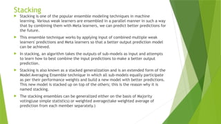
 Stacking is one of the popular ensemble modeling techniques in machine
learning. Various weak learners are ensembled in a parallel manner in such a way
that by combining them with Meta learners, we can predict better predictions for
the future.
 This ensemble technique works by applying input of combined multiple weak
learners' predictions and Meta learners so that a better output prediction model
can be achieved.
 In stacking, an algorithm takes the outputs of sub-models as input and attempts
to learn how to best combine the input predictions to make a better output
prediction.
 Stacking is also known as a stacked generalization and is an extended form of the
Model Averaging Ensemble technique in which all sub-models equally participate
as per their performance weights and build a new model with better predictions.
This new model is stacked up on top of the others; this is the reason why it is
named stacking.
 The stacking ensembles can be generalized either on the basis of Majority
voting(use simple statistics) or weighted average(take weighted average of
prediction from each member separately.)

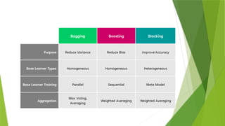
58. Random forest
 Random Forest Models can be thought of as BAGGing, with a slight tweak.
When deciding where to split and how to make decisions, BAGGed
Decision Trees have the full disposal of features to choose from. Therefore,
although the bootstrapped samples may be slightly different, the data is
largely going to break off at the same features throughout each model.
 In contrary, Random Forest models decide where to split based on a
random selection of features. Rather than splitting at similar features at
each node throughout, Random Forest models implement a level of
differentiation because each tree will split based on different features.
 This level of differentiation provides a greater ensemble to aggregate over,
ergo producing a more accurate predictor.
 Similar to BAGGing, bootstrapped subsamples are pulled from a larger
dataset. A decision tree is formed on each subsample. HOWEVER, the
decision tree is split on different features (in this diagram the features are
represented by shapes).
 Random Forest is a classifier that contains a number of decision trees on
various subsets of the given dataset and takes the average to improve the
predictive accuracy of that dataset.
 The greater number of trees in the forest leads to higher accuracy and
prevents the problem of overfitting.

59.  Why use Random Forest?
• It takes less training time as compared to other algorithms.
• It predicts output with high accuracy, even for the large dataset it runs
efficiently.
• It can also maintain accuracy when a large proportion of data is missing.
 How does Random Forest algorithm work?
 Random Forest works in two-phase first is to create the random forest by
combining N decision tree, and second is to make predictions for each tree
created in the first phase.
 The Working process can be explained in the below steps and diagram:
 Step-1: Select random K data points from the training set.
 Step-2: Build the decision trees associated with the selected data points
(Subsets).
 Step-3: Choose the number N for decision trees that you want to build.
 Step-4: Repeat Step 1 & 2.
 Step-5: For new data points, find the predictions of each decision tree, and
assign the new data points to the category that wins the majority votes.

60.  from sklearn.ensemble import RandomForestClassifier
 import pandas as pd
 import matplotlib.pyplot as plt
iris = pd.read_csv("/content/drive/MyDrive/Colab Notebooks/ML BCA SEM 5/iris_dataset.csv")
 print(iris.head(5))
 print(iris.columns)
 X=iris.drop('target',axis=1)
 y=iris['target']
print(y.value_counts())
clf = RandomForestClassifier(n_estimators=5,criterion="entropy") #no. of esimators is number of trees
used
 clf = clf.fit(X.values, y)
 clf.predict([[3.4,4.5,3.1,6.2]])