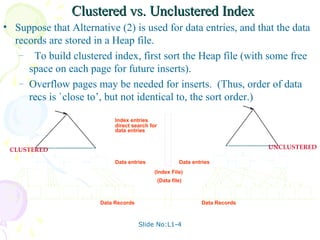
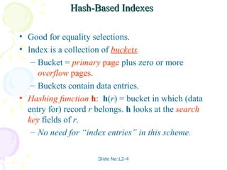
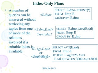
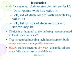
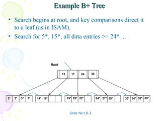
Indexing is used to speed up access to desired data.
E.g. author catalog in library
A search key is an attribute or set of attributes used to look up records in a file. Unrelated to keys in the db schema.
An index file consists of records called index entries.
An index entry for key k may consist of
An actual data record (with search key value k)
A pair (k, rid) where rid is a pointer to the actual data record
A pair (k, bid) where bid is a pointer to a bucket of record pointers
Index files are typically much smaller than the original file if the actual data records are in a separate file.
If the index contains the data records, there is a single file with a special organization.
ADVANCE DATABASE MANAGEMENT SYSTEM CONCEPTS & ARCHITECTURE by vikas jagtapVikas Jagtap
The data that indicates the earth location (latitude & longitude, or height & depth ) of these rendered objects is known as spatial data.
When the map is rendered, objects of this spatial data are used to project the location of the objects on 2-Dimentional piece of paper.
The spatial data management systems are designed to make the storage, retrieval, & manipulation of spatial data (i.e points, lines and polygons) easier and natural to users, such as GIS.
While typical databases can understand various numeric and character types of data, additional functionality needs to be added for databases to process spatial data types.
These are typically called geometry or feature.
In this talk we will discuss what happens to data when it is written from the HDF5 application to an HDF5 file. This knowledge will help developers to write more efficient applications and to avoid performance bottlenecks.
JMeter webinar - integration with InfluxDB and GrafanaRTTS
Watch this recorded webinar about real-time monitoring of application performance. See how to integrate Apache JMeter, the open-source leader in performance testing, with InfluxDB, the open-source time-series database, and Grafana, the open-source analytics and visualization application.
In this webinar, we will review the benefits of leveraging InfluxDB and Grafana when executing load tests and demonstrate how these tools are used to visualize performance metrics.
Length: 30 minutes
Session Overview
-------------------------------------------
During this webinar, we will cover the following topics while demonstrating the integrations of JMeter, InfluxDB and Grafana:
- What out-of-the-box solutions are available for real-time monitoring JMeter tests?
- What are the benefits of integrating InfluxDB and Grafana into the load testing stack?
- Which features are provided by Grafana?
- Demonstration of InfluxDB and Grafana using a practice web application
To view the webinar recording, go to:
https://www.rttsweb.com/jmeter-integration-webinar
Smart TV Buyer Insights Survey 2024 by 91mobiles.pdf91mobiles
91mobiles recently conducted a Smart TV Buyer Insights Survey in which we asked over 3,000 respondents about the TV they own, aspects they look at on a new TV, and their TV buying preferences.
LF Energy Webinar: Electrical Grid Modelling and Simulation Through PowSyBl -...DanBrown980551
Do you want to learn how to model and simulate an electrical network from scratch in under an hour?
Then welcome to this PowSyBl workshop, hosted by Rte, the French Transmission System Operator (TSO)!
During the webinar, you will discover the PowSyBl ecosystem as well as handle and study an electrical network through an interactive Python notebook.
PowSyBl is an open source project hosted by LF Energy, which offers a comprehensive set of features for electrical grid modelling and simulation. Among other advanced features, PowSyBl provides:
- A fully editable and extendable library for grid component modelling;
- Visualization tools to display your network;
- Grid simulation tools, such as power flows, security analyses (with or without remedial actions) and sensitivity analyses;
The framework is mostly written in Java, with a Python binding so that Python developers can access PowSyBl functionalities as well.
What you will learn during the webinar:
- For beginners: discover PowSyBl's functionalities through a quick general presentation and the notebook, without needing any expert coding skills;
- For advanced developers: master the skills to efficiently apply PowSyBl functionalities to your real-world scenarios.
Neuro-symbolic is not enough, we need neuro-*semantic*Frank van Harmelen
Neuro-symbolic (NeSy) AI is on the rise. However, simply machine learning on just any symbolic structure is not sufficient to really harvest the gains of NeSy. These will only be gained when the symbolic structures have an actual semantics. I give an operational definition of semantics as “predictable inference”.
All of this illustrated with link prediction over knowledge graphs, but the argument is general.
Software Delivery At the Speed of AI: Inflectra Invests In AI-Powered QualityInflectra
In this insightful webinar, Inflectra explores how artificial intelligence (AI) is transforming software development and testing. Discover how AI-powered tools are revolutionizing every stage of the software development lifecycle (SDLC), from design and prototyping to testing, deployment, and monitoring.
Learn about:
• The Future of Testing: How AI is shifting testing towards verification, analysis, and higher-level skills, while reducing repetitive tasks.
• Test Automation: How AI-powered test case generation, optimization, and self-healing tests are making testing more efficient and effective.
• Visual Testing: Explore the emerging capabilities of AI in visual testing and how it's set to revolutionize UI verification.
• Inflectra's AI Solutions: See demonstrations of Inflectra's cutting-edge AI tools like the ChatGPT plugin and Azure Open AI platform, designed to streamline your testing process.
Whether you're a developer, tester, or QA professional, this webinar will give you valuable insights into how AI is shaping the future of software delivery.
UiPath Test Automation using UiPath Test Suite series, part 4DianaGray10
Welcome to UiPath Test Automation using UiPath Test Suite series part 4. In this session, we will cover Test Manager overview along with SAP heatmap.
The UiPath Test Manager overview with SAP heatmap webinar offers a concise yet comprehensive exploration of the role of a Test Manager within SAP environments, coupled with the utilization of heatmaps for effective testing strategies.
Participants will gain insights into the responsibilities, challenges, and best practices associated with test management in SAP projects. Additionally, the webinar delves into the significance of heatmaps as a visual aid for identifying testing priorities, areas of risk, and resource allocation within SAP landscapes. Through this session, attendees can expect to enhance their understanding of test management principles while learning practical approaches to optimize testing processes in SAP environments using heatmap visualization techniques
What will you get from this session?
1. Insights into SAP testing best practices
2. Heatmap utilization for testing
3. Optimization of testing processes
4. Demo
Topics covered:
Execution from the test manager
Orchestrator execution result
Defect reporting
SAP heatmap example with demo
Speaker:
Deepak Rai, Automation Practice Lead, Boundaryless Group and UiPath MVP
State of ICS and IoT Cyber Threat Landscape Report 2024 previewPrayukth K V
The IoT and OT threat landscape report has been prepared by the Threat Research Team at Sectrio using data from Sectrio, cyber threat intelligence farming facilities spread across over 85 cities around the world. In addition, Sectrio also runs AI-based advanced threat and payload engagement facilities that serve as sinks to attract and engage sophisticated threat actors, and newer malware including new variants and latent threats that are at an earlier stage of development.
The latest edition of the OT/ICS and IoT security Threat Landscape Report 2024 also covers:
State of global ICS asset and network exposure
Sectoral targets and attacks as well as the cost of ransom
Global APT activity, AI usage, actor and tactic profiles, and implications
Rise in volumes of AI-powered cyberattacks
Major cyber events in 2024
Malware and malicious payload trends
Cyberattack types and targets
Vulnerability exploit attempts on CVEs
Attacks on counties – USA
Expansion of bot farms – how, where, and why
In-depth analysis of the cyber threat landscape across North America, South America, Europe, APAC, and the Middle East
Why are attacks on smart factories rising?
Cyber risk predictions
Axis of attacks – Europe
Systemic attacks in the Middle East
Download the full report from here:
https://sectrio.com/resources/ot-threat-landscape-reports/sectrio-releases-ot-ics-and-iot-security-threat-landscape-report-2024/
Dev Dives: Train smarter, not harder – active learning and UiPath LLMs for do...UiPathCommunity
💥 Speed, accuracy, and scaling – discover the superpowers of GenAI in action with UiPath Document Understanding and Communications Mining™:
See how to accelerate model training and optimize model performance with active learning
Learn about the latest enhancements to out-of-the-box document processing – with little to no training required
Get an exclusive demo of the new family of UiPath LLMs – GenAI models specialized for processing different types of documents and messages
This is a hands-on session specifically designed for automation developers and AI enthusiasts seeking to enhance their knowledge in leveraging the latest intelligent document processing capabilities offered by UiPath.
Speakers:
👨🏫 Andras Palfi, Senior Product Manager, UiPath
👩🏫 Lenka Dulovicova, Product Program Manager, UiPath
Builder.ai Founder Sachin Dev Duggal's Strategic Approach to Create an Innova...Ramesh Iyer
In today's fast-changing business world, Companies that adapt and embrace new ideas often need help to keep up with the competition. However, fostering a culture of innovation takes much work. It takes vision, leadership and willingness to take risks in the right proportion. Sachin Dev Duggal, co-founder of Builder.ai, has perfected the art of this balance, creating a company culture where creativity and growth are nurtured at each stage.
"Impact of front-end architecture on development cost", Viktor TurskyiFwdays
I have heard many times that architecture is not important for the front-end. Also, many times I have seen how developers implement features on the front-end just following the standard rules for a framework and think that this is enough to successfully launch the project, and then the project fails. How to prevent this and what approach to choose? I have launched dozens of complex projects and during the talk we will analyze which approaches have worked for me and which have not.
GraphRAG is All You need? LLM & Knowledge GraphGuy Korland
Guy Korland, CEO and Co-founder of FalkorDB, will review two articles on the integration of language models with knowledge graphs.
1. Unifying Large Language Models and Knowledge Graphs: A Roadmap.
https://arxiv.org/abs/2306.08302
2. Microsoft Research's GraphRAG paper and a review paper on various uses of knowledge graphs:
https://www.microsoft.com/en-us/research/blog/graphrag-unlocking-llm-discovery-on-narrative-private-data/
FIDO Alliance Osaka Seminar: The WebAuthn API and Discoverable Credentials.pdf
Unit 08 dbms
1. DATABASE MANAGEMENT SYSTEMS
MALLA REDDY ENGG. COLLEGE HYD
II B. Tech CSE II Semester
UNIT-VIII PPT SLIDES
Text Books: (1) DBMS by Raghu Ramakrishnan
(2) DBMS by Sudarshan and Korth
2. INDEX
UNIT-8 PPT SLIDES
S.NO Module as per Lecture PPT
Session planner No Slide NO
-------------------------------------------------------------------------------------------------
1. Data on external storage &
File organization and indexing L1 L1- 1 to L1- 4
2. Index data structures L2 L2- 1 to L2- 7
3. Comparison of file organizations L3 L3- 1 to L3- 5
4. Comparison of file organizations L4 L4- 1 to L4- 2
5. Indexes and performance tuning L5 L5- 1 to L5- 4
6. Indexes and performance tuning L6 L6- 1 to L6 -5
7. Intuition for tree indexes & ISAM L7 L7- 1 to L7- 7
8. B+ tree L8 L8- 1 to L8- 9
3. Data on External Storage
• Disks: Can retrieve random page at fixed cost
– But reading several consecutive pages is much cheaper
than reading them in random order
• Tapes: Can only read pages in sequence
– Cheaper than disks; used for archival storage
• File organization: Method of arranging a file of records on
external storage.
– Record id (rid) is sufficient to physically locate record
– Indexes are data structures that allow us to find the record
ids of records with given values in index search key fields
• Architecture: Buffer manager stages pages from external
storage to main memory buffer pool. File and index layers
make calls to the buffer manager.
Slide No:L1-1
4. Alternative File Organizations
Many alternatives exist, each ideal for some situations, and
not so good in others:
– Heap (random order) files: Suitable when typical access
is a file scan retrieving all records.
– Sorted Files: Best if records must be retrieved in some
order, or only a `range’ of records is needed.
– Indexes: Data structures to organize records via trees or
hashing.
• Like sorted files, they speed up searches for a subset
of records, based on values in certain (“search key”)
fields
• Updates are much faster than in sorted files.
Slide No:L1-2
5. Index Classification
• Primary vs. secondary: If search key contains primary
key, then called primary index.
– Unique index: Search key contains a candidate key.
• Clustered vs. unclustered: If order of data records is
the same as, or `close to’, order of data entries, then
called clustered index.
– Alternative 1 implies clustered; in practice,
clustered also implies Alternative 1 (since sorted
files are rare).
– A file can be clustered on at most one search key.
– Cost of retrieving data records through index varies
greatly based on whether index is clustered or not!
Slide No:L1-3
6. Clustered vs. Unclustered Index
• Suppose that Alternative (2) is used for data entries, and that the data
records are stored in a Heap file.
– To build clustered index, first sort the Heap file (with some free
space on each page for future inserts).
– Overflow pages may be needed for inserts. (Thus, order of data
recs is `close to’, but not identical to, the sort order.)
Index entries
direct search for
data entries
CLUSTERED UNCLUSTERED
Data entries Data entries
(Index File)
(Data file)
Data Records Data Records
Slide No:L1-4
7. Indexes
• An index on a file speeds up selections on the
search key fields for the index.
– Any subset of the fields of a relation can be the
search key for an index on the relation.
– Search key is not the same as key (minimal set
of fields that uniquely identify a record in a
relation).
• An index contains a collection of data entries, and
supports efficient retrieval of all data entries k*
with a given key value k.
– Given data entry k*, we can find record with
key k in at most one disk I/O. (Details soon …)
Slide No:L2-1
8. B+ Tree Indexes
Non-leaf
Pages
Leaf
Pages
(Sorted by search key)
Leaf pages contain data entries, and are chained (prev & next)
Non-leaf pages have index entries; only used to direct searches:
index entry
P0 K 1 P1 K 2 P 2 K m Pm
Slide No:L2-2
9. Example B+ Tree
Root Note how data entries
17 in leaf level are sorted
Entries <= 17 Entries > 17
5 13 27 30
2* 3* 5* 7* 8* 14* 16* 22* 24* 27* 29* 33* 34* 38* 39*
• Find 28*? 29*? All > 15* and < 30*
• Insert/delete: Find data entry in leaf, then change
it. Need to adjust parent sometimes.
– And change sometimes bubbles up the tree
Slide No:L2-3
10. Hash-Based Indexes
• Good for equality selections.
• Index is a collection of buckets.
– Bucket = primary page plus zero or more
overflow pages.
– Buckets contain data entries.
• Hashing function h: h(r) = bucket in which (data
entry for) record r belongs. h looks at the search
key fields of r.
– No need for “index entries” in this scheme.
Slide No:L2-4
11. Alternatives for Data Entry k* in Index
• In a data entry k* we can store:
– Data record with key value k, or
– <k, rid of data record with search key value k>, or
– <k, list of rids of data records with search key k>
• Choice of alternative for data entries is orthogonal to
the indexing technique used to locate data entries with
a given key value k.
– Examples of indexing techniques: B+ trees, hash-
based structures
– Typically, index contains auxiliary information
that directs searches to the desired data entries
Slide No:L2-5
12. Alternatives for Data Entries (Contd.)
• Alternative 1:
– If this is used, index structure is a file
organization for data records (instead of a Heap
file or sorted file).
– At most one index on a given collection of data
records can use Alternative 1. (Otherwise, data
records are duplicated, leading to redundant
storage and potential inconsistency.)
– If data records are very large, # of pages
containing data entries is high. Implies size of
auxiliary information in the index is also large,
typically.
Slide No:L2-6
13. Alternatives for Data Entries (Contd.)
• Alternatives 2 and 3:
– Data entries typically much smaller than data
records. So, better than Alternative 1 with large
data records, especially if search keys are small.
(Portion of index structure used to direct search,
which depends on size of data entries, is much
smaller than with Alternative 1.)
– Alternative 3 more compact than Alternative 2,
but leads to variable sized data entries even if
search keys are of fixed length.
Slide No:L2-7
14. Cost Model for Our Analysis
We ignore CPU costs, for simplicity:
– B: The number of data pages
– R: Number of records per page
– D: (Average) time to read or write
disk page
– Measuring number of page I/O’s
ignores gains of pre-fetching a
sequence of pages; thus, even I/O cost
is only approximated.
– Average-case analysis; based on
several simplistic assumptions.
Slide No:L3-1
15. Comparing File Organizations
• Heap files (random order; insert at eof)
• Sorted files, sorted on <age, sal>
• Clustered B+ tree file, Alternative (1), search key
<age, sal>
• Heap file with unclustered B + tree index on search
key <age, sal>
• Heap file with unclustered hash index on search key
<age, sal>
Slide No:L3-2
16. Operations to Compare
• Scan: Fetch all records from disk
• Equality search
• Range selection
• Insert a record
• Delete a record
Slide No:L3-3
17. Assumptions in Our Analysis
• Heap Files:
– Equality selection on key; exactly one match.
• Sorted Files:
– Files compacted after deletions.
• Indexes:
– Alt (2), (3): data entry size = 10% size of
record
– Hash: No overflow buckets.
• 80% page occupancy => File size = 1.25
data size
– Tree: 67% occupancy (this is typical).
• Implies file size = 1.5 data size
Slide No:L3-4
18. Assumptions (contd.)
• Scans:
– Leaf levels of a tree-index are chained.
– Index data-entries plus actual file
scanned for unclustered indexes.
• Range searches:
– We use tree indexes to restrict the set
of data records fetched, but ignore hash
indexes.
Slide No:L3-5
19. Cost of Operations
(a) Scan (b) Equality (c ) Range (d) Insert (e) Delete
(1) Heap BD 0.5BD BD 2D Search
+D
(2) Sorted BD Dlog 2B D(log 2 B + Search Search
# pgs with + BD +BD
match recs)
(3) 1.5BD Dlog F 1.5B D(log F 1.5B Search Search
Clustered + # pgs w. +D +D
match recs)
(4) Unclust. BD(R+0.15) D(1 + D(log F 0.15B Search Search
Tree index log F 0.15B) + # pgs w. + 2D + 2D
match recs)
(5) Unclust. BD(R+0.125) 2D BD Search Search
Hash index + 2D + 2D
Slide No:L4-1
20. Understanding the Workload
• For each query in the workload:
– Which relations does it access?
– Which attributes are retrieved?
– Which attributes are involved in selection/join
conditions? How selective are these conditions
likely to be?
• For each update in the workload:
– Which attributes are involved in selection/join
conditions? How selective are these conditions
likely to be?
– The type of update (INSERT/DELETE/UPDATE), and
the attributes that are affected.
Slide No:L4-2
21. Choice of Indexes
• What indexes should we create?
– Which relations should have indexes?
What field(s) should be the search
key? Should we build several indexes?
• For each index, what kind of an index should it be?
– Clustered? Hash/tree?
Slide No:L5-1
22. Choice of Indexes (Contd.)
• One approach: Consider the most important queries in turn. Consider
the best plan using the current indexes, and see if a better plan is
possible with an additional index. If so, create it.
– Obviously, this implies that we must understand
how a DBMS evaluates queries and creates query
evaluation plans!
– For now, we discuss simple 1-table queries.
• Before creating an index, must also consider the impact on updates in
the workload!
– Trade-off: Indexes can make queries go faster,
updates slower. Require disk space, too.
Slide No:L5-2
23. Index Selection Guidelines
• Attributes in WHERE clause are candidates for index keys.
– Exact match condition suggests hash index.
– Range query suggests tree index.
• Clustering is especially useful for range
queries; can also help on equality queries if
there are many duplicates.
• Multi-attribute search keys should be considered when a WHERE
clause contains several conditions.
– Order of attributes is important for range queries.
– Such indexes can sometimes enable index-only
strategies for important queries.
• For index-only strategies, clustering is not
important!
Slide No:L5-3
24. Examples of Clustered Indexes
• B+ tree index on E.age can be used to get SELECT E.dno
qualifying tuples. FROM Emp E
– How selective is the condition? WHERE E.age>40
– Is the index clustered?
SELECT E.dno, COUNT (*)
• Consider the GROUP BY query. FROM Emp E
– If many tuples have E.age > 10, WHERE E.age>10
using E.age index and sorting GROUP BY E.dno
the retrieved tuples may be
costly.
– Clustered E.dno index may be
better!
• Equality queries and duplicates: SELECT E.dno
– Clustering on E.hobby helps! FROM Emp E
Slide No:L5-4 WHERE E.hobby=Stamps
25. Indexes with Composite Search Keys
• Composite Search Keys: Search on a
Examples of composite key
combination of fields.
indexes using lexicographic order.
– Equality query: Every field
value is equal to a
constant value. E.g. wrt
<sal,age> index:
• age=20 and sal =75 11,80 11
12,10 12
– Range query: Some field name age sal
12,20 12
value is not a constant. 13,75 bob 12 10 13
E.g.: <age, sal> cal 11 80 <age>
• age =20; or age=20 joe 12 20
and sal > 10 10,12 sue 13 75 10
20,12 20
• Data entries in index sorted by Data records
75,13 sorted by name 75
search key to support range queries.
80,11 80
– Lexicographic order, or
<sal, age> <sal>
– Spatial order. Data entries in index Data entries
sorted by <sal,age> sorted by <sal>
Slide No:L6-1
26. Composite Search Keys
• To retrieve Emp records with age=30 AND sal=4000, an
index on <age,sal> would be better than an index on age or an
index on sal.
– Choice of index key orthogonal to clustering
etc.
• If condition is: 20<age<30 AND 3000<sal<5000:
– Clustered tree index on <age,sal> or
<sal,age> is best.
• If condition is: age=30 AND 3000<sal<5000:
– Clustered <age,sal> index much better than
<sal,age> index!
• Composite indexes are larger, updated more often.
Slide No:L6-2
27. Index-Only Plans
• A number of SELECT E.dno, COUNT(*)
queries can be <E.dno> FROM Emp E
GROUP BY E.dno
answered without
retrieving any
tuples from one <E.dno,E.sal> SELECT E.dno, MIN(E.sal)
or more of the FROM Emp E
Tree index!
relations GROUP BY E.dno
involved if a
suitable index is
<E. age,E.sal> SELECT AVG(E.sal)
available. or FROM Emp E
<E.sal, E.age> WHERE E.age=25 AND
Tree index!
E.sal BETWEEN 3000 AND 5000
Slide No:L6-3
28. Summary
• Many alternative file organizations exist, each
appropriate in some situation.
• If selection queries are frequent, sorting the file or
building an index is important.
– Hash-based indexes only good for
equality search.
– Sorted files and tree-based indexes best
for range search; also good for equality
search. (Files rarely kept sorted in
practice; B+ tree index is better.)
• Index is a collection of data entries plus a way to
quickly find entries with given key values.
Slide No:L6-4
29. Summary (Contd.)
• Data entries can be actual data records, <key, rid>
pairs, or <key, rid-list> pairs.
– Choice orthogonal to indexing
technique used to locate data entries
with a given key value.
• Can have several indexes on a given file of data
records, each with a different search key.
• Indexes can be classified as clustered vs.
unclustered, primary vs. secondary, and dense vs.
sparse. Differences have important consequences
for utility/performance.
Slide No:L6-5
30. Introduction
• As for any index, 3 alternatives for data entries k*:
– Data record with key value k
– <k, rid of data record with search key
value k>
– <k, list of rids of data records with
search key k>
• Choice is orthogonal to the indexing technique used
to locate data entries k*.
• Tree-structured indexing techniques support both
range searches and equality searches.
• ISAM: static structure; B+ tree: dynamic, adjusts
gracefully under inserts and deletes.
Slide No:L7-1
31. Range Searches
• ``Find all students with gpa > 3.0’’
– If data is in sorted file, do binary
search to find first such student, then
scan to find others.
– Cost of binary search can be quite
high.
• Simple idea: Create an `index’ file.
k1 k2 kN Index File
Page 1 Page 2 Page 3 Page N Data File
Slide No:L7-2
32. index entry
ISAM
P K P K 2 P K m Pm
0 1 1 2
• Index file may still be quite large. But we can apply
the idea repeatedly!
Non-leaf
Pages
Leaf
Pages
Overflow
page
Primary pages
Slide No:L7-3
33. Comments on ISAM
Data
Pages
• File creation: Leaf (data) pages allocated
sequentially, sorted by search key; then index
pages allocated, then space for overflow pages. Index Pages
• Index entries: <search key value, page id>; they
`direct’ search for data entries, which are in leaf
pages. Overflow pages
• Search: Start at root; use key comparisons to go
to leaf. Cost log F N ; F = # entries/index pg, N
= # leaf pgs
∝
• Insert: Find leaf data entry belongs to, and put it
there.
• Delete: Find and remove from leaf; if empty
overflow page, de-allocate.
Slide No:L7-4
34. Example ISAM Tree
• Each node can hold 2 entries; no need for `next-leaf-
page’ pointers. (Why?)
Root
40
20 33 51 63
10* 15* 20* 27* 33* 37* 40* 46* 51* 55* 63* 97*
Slide No:L7-5
37. B+ Tree: Most Widely Used Index
• Insert/delete at log F N cost; keep tree height-balanced.
(F = fanout, N = # leaf pages)
• Minimum 50% occupancy (except for root). Each
node contains d <= m <= 2d entries. The parameter
d is called the order of the tree.
• Supports equality and range-searches efficiently.
Index Entries
(Direct search)
Data Entries
("Sequence set")
Slide No:L8-1
38. Example B+ Tree
• Search begins at root, and key comparisons direct it
to a leaf (as in ISAM).
• Search for 5*, 15*, all data entries >= 24* ...
Root
13 17 24 30
2* 3* 5* 7* 14* 16* 19* 20* 22* 24* 27* 29* 33* 34* 38* 39*
Slide No:L8-2
39. B+ Trees in Practice
• Typical order: 100. Typical fill-factor: 67%.
– average fanout = 133
• Typical capacities:
– Height 4: 1334 = 312,900,700 records
– Height 3: 1333 = 2,352,637 records
• Can often hold top levels in buffer pool:
– Level 1 = 1 page = 8 Kbytes
– Level 2 = 133 pages = 1 Mbyte
– Level 3 = 17,689 pages = 133 MBytes
Slide No:L8-3
40. Inserting a Data Entry into a B+ Tree
• Find correct leaf L.
• Put data entry onto L.
– If L has enough space, done!
– Else, must split L (into L and a new node L2)
• Redistribute entries evenly, copy up middle
key.
• Insert index entry pointing to L2 into parent
of L.
• This can happen recursively
– To split index node, redistribute entries evenly,
but push up middle key. (Contrast with leaf
splits.)
• Splits “grow” tree; root split increases height.
– Tree growth: gets wider or one level taller at
top. Slide No:L8-4
41. Inserting 8* into Example B+ Tree
Entry to be inserted in parent node.
• Observe how 5 (Note that 5 is copied up and
s
continues to appear in the leaf.)
minimum
occupancy is
2* 3* 5* 7* 8*
guaranteed in
both leaf and
index pg splits.
• Note difference Entry to be inserted in parent node.
(Note that 17 is pushed up and only
between copy-up 17
appears once in the index. Contrast
this with a leaf split.)
and push-up; be
sure you 5 13 24 30
understand the
reasons for this.
Slide No:L8-5
42. Example B+ Tree After Inserting 8*
Root
17
5 13 24 30
2* 3* 5* 7* 8* 14* 16* 19* 20* 22* 24* 27* 29* 33* 34* 38* 39*
Notice that root was split, leading to increase in height.
In this example, we can avoid split by re-distributing
entries; however, this is usually not done in practice.
Slide No:L8-6
43. Deleting a Data Entry from a B+ Tree
• Start at root, find leaf L where entry belongs.
• Remove the entry.
– If L is at least half-full, done!
– If L has only d-1 entries,
• Try to re-distribute, borrowing from sibling
(adjacent node with same parent as L).
• If re-distribution fails, merge L and sibling.
• If merge occurred, must delete entry (pointing to L or sibling)
from parent of L.
• Merge could propagate to root, decreasing height.
Slide No:L8-7
44. Example Tree After (Inserting 8*, Then)
Deleting 19* and 20* ...
Root
17
5 13 27 30
2* 3* 5* 7* 8* 14* 16* 22* 24* 27* 29* 33* 34* 38* 39*
• Deleting 19* is easy.
• Deleting 20* is done with re-distribution. Notice
how middle key is copied up.
Slide No:L8-8
45. ... And Then Deleting 24*
• Must merge.
30
• Observe `toss’ of index
entry (on right), and 22* 27* 38* 39*
29* 33* 34*
`pull down’ of index
entry (below).
Root
5 13 17 30
2* 3* 5* 7* 8* 14* 16* 22* 27* 29* 33* 34* 38* 39*
Slide No:L8-9