The document discusses file organization and indexing methods in database management systems, covering various indexing techniques including clustered and unclustered indexes, tree-based indexing, and hash-based indexing. It details data structures such as B+ trees and ISAM, explaining how they facilitate efficient data retrieval and management through structured record identification and access methods. Additionally, it compares different file organizational techniques and their impact on performance during operations like scanning, searching, inserting, and deleting records.

1. Data on External Storage
– File Organization and Indexing
– Cluster Indexes
- Primary and Secondary Indexes
– Index data Structures
– Hash Based Indexing
– Tree base Indexing
– Comparison of File Organizations
– Indexes and Performance Tuning
- Intuitions for tree Indexes
– Indexed Sequential Access Methods (ISAM)
– B+ Trees: A Dynamic Index Structure.
UNIT VI

2. FILE: The basic abstraction of data in a DBMS is a collection
of records, or a file and each of consists of one or more pages.
FILES AND ACCESS METHODS LAYER organizes data
to support fast accessing the data.
FILE ORGANIZATION is a method of arranging the records
in a file when the file is stored on disk.
The unit of information read from or written to disk is a page.
Typically the size of a page is 4kb or 8kb.

3. Data on External Storage
Storage: offer persistent data storage, data saved on a persistent
storage is not lost when the system shutdowns or crashes.
Disks: Can retrieve random page at fixed cost. But reading several
consecutive pages is much cheaper than reading them in random
Order.
Tapes: Can only read pages in sequence. Cheaper than disks;
used for archival storage.
Other types of persistent storage devices: Optical storage, Flash
Memory.
Each record in a file has a unique identifier called a record id or
rid.

4. Layered Architecture
Disk Space Manager allocates/de-
allocates spaces on disks.
Buffer manager moves pages between
disks and main memory.
File and index layers organize records on
files, and manage the indexing data
structure.

5. File Organization
Method of arranging a file of records on external storage.
Different alternatives
1. Heap files: Records are unsorted.
Suitable when typical access is a file scan retrieving all records without any
order. Fast update (insertions / deletions)
2. Sorted Files: Records are sorted.
Best if records must be retrieved in some order, or only a `range’ of records
is needed.
Examples: employees are sorted by age.
Slow update in comparison to heap file.
3. Indexes: Data structures to organize records via trees or hashing.
For example, create an index on employee age.
Like sorted files, speed up searches for a subset of records that match values
in certain (“search key”) fields
Updates are much faster than in sorted files.

6. Indexes
An index on a file speeds up selections on the search key fields for the
index.
Any subset of the attributes of a table can be the search key for an
index on the relation.
Search key does not have to be candidate key
Example: employee age is not a candidate key.
An index file contains a collection of data entries (called k*).
Quickly search an index to locate a data entry with a key value k.

7. Indexes(contd..)
Three alternatives for what to store in a data entry:
Alternative 1: Data record with key value k
Example data record = data entry: <age, name, salary>
Alternative 2: <k, rid of data record with search key value k>
Example data entry: <age, rid>
Alternative 3: <k, list of rids of data records with search key k>
Example data entry: <age, rid_1, rid_2, …>
Indexing method takes a search key and finds the data entries matching
the search key.
Examples of indexing methods: B+ trees or hashing.

8. Typical Index Architecture
(Data file)
Data entries
Data Records
(Index File)
k* k* k*
Search structure: given a key, it finds the
data entry for that key

9. Index Classification
Clustered index and Unclustered:
If order of data records is the same as, or close to the order of data entries,
then it is called clustered index otherwise it is unclustered index.
Why is this important?
Cost of retrieving data records through index varies greatly based on
whether index is clustered or not!
Consider the cost of range search query: find all records 30<age<39
Primary and secondary indexes:
An index on a set of fields that includes the primary key is called primary
index; otherwise indexes are called secondary indexes.

10. Clustered Vs Unclustered Index
CLUSTERED
Index entries
Data entries
direct search for
(Index File)
Data Records
data entries
(Data file)
Data entries
Data Records
UNCLUSTERED

11. Index Data Structures
 Hash-based indexing, Tree-based indexing
Hash-based indexing:
Good for equality selections.
Index is a collection of buckets.
Bucket = primary page plus zero or more overflow pages.
Buckets contain data entries.
Hashing function h: h(r) = bucket in which record r belongs. h
looks at the search key fields of r.

12. Hash-based Index Examples
age
sal
h
Smith,44,3000
Jones,40,6003
Tracy,44,5004
Ashby,25,3000
Basu,33,4003
Bristow,29,2007
Cass,50,5004
Daniels,22,6003
h(age)=00
h(age)=01
h(age)=10
3000
3000
5004
5004
4003
2007
6003
6003
h
h(sal)=00
h(sal)=11
Employees file hashed on age Index on salary

13. Hash-based indexing(contd..)
Search on key value:
– Apply key value to the hash function -> bucket number
– Retrieve the primary page of the bucket. Search records in the
primary page. If not found, search the overflow pages.
– Cost of locating rids: # pages in bucket (small)
Insert a record:
– Apply key value to the hash function -> bucket number
– If all (primary & overflow) pages in that bucket are full, allocate
a new overflow page.
– Cost: similar to search.
Delete a record
– Cost: Similar to search.

14. Static Hashing
# primary pages fixed, allocated sequentially, never
de-allocated; overflow pages if needed.
h(k) mod N = bucket to which data entry with key k
belongs. (N = # of buckets).
Primary bucket pages Overflow pages
h(key) mod N
h
key
2
0
N-1

15. Static Hashing(Contd.)
Buckets contain data entries.
Hash fn works on search key field of record r.
Long overflow chains can develop and degrade performance.
Extendible and Linear Hashing: Dynamic techniques to fix this
problem.

16. Extendible Hashing
Situation: Bucket (primary page) becomes full. Why not re-
organize file by doubling # of buckets?
Reading and writing all pages is expensive!
Idea: Use directory of pointers to buckets, double # of
buckets by doubling the directory, splitting just the bucket
that overflowed!
Directory much smaller than file, so doubling it is much
cheaper. Only one page of data entries is split. No overflow
Page!

17. Example
Directory is array of size 4.
To find bucket for r, take last
`global depth’ # bits of h(r); we
denote r by h(r).
If h(r) = 5 = binary 101, it is in
bucket pointed to by 01.
Insert: If bucket is full, split it (allocate new page, re-distribute).
If necessary, double the directory.
13*
00
01
10
11
2
2
2
2
2
LOCAL DEPTH
GLOBAL DEPTH
DIRECTORY
Bucket A
Bucket B
Bucket C
Bucket D
DATA PAGES
10*
1* 21*
4* 12* 32* 16*
15* 7* 19*
5*

18. Insert h(r)=20 (Causes Doubling)
20*
00
01
10
11
2 2
2
2
LOCAL DEPTH 2
2
DIRECTORY
GLOBAL DEPTH
Bucket A
Bucket B
Bucket C
Bucket D
Bucket A2
(`split image'
of Bucket A)
1* 5* 21*13*
32*16*
10*
15* 7* 19*
4* 12*
19*
2
2
2
000
001
010
011
100
101
110
111
3
3
3
DIRECTORY
Bucket A
Bucket B
Bucket C
Bucket D
Bucket A2
(`split image'
of Bucket A)
32*
1* 5* 21*13*
16*
10*
15* 7*
4* 20*
12*
LOCAL DEPTH
GLOBAL DEPTH

19. Points to Remember
20 = binary 10100. Last 2 bits (00) tell us r belongs in A or A2.
Last 3 bits needed to tell which.
Global depth of directory: Max # of bits needed to tell which
bucket an entry belongs to.
Local depth of a bucket: # of bits used to determine if an entry
belongs to this bucket.

20. Tree-based Indexing
Tree-structured indexing techniques support both
range searches and equality searches
Types :
ISAM: static structure,
B+ tree: dynamic structure.

21. Indexed Sequential Access Method(ISAM)
File creation: Leaf (data) pages allocated sequentially, sorted
by search key; then index pages allocated, then space for
overflow pages.
Index entries: <search key value, page id>; they `direct’
search for data entries, which are in leaf pages.
Search: Start at root; use key comparisons to go to leaf. Cost
log F N ; F = # pointers/index pg, N = # leaf pgs
Insert: Find leaf that data entry belongs to, and put it there,
which may be in the primary or overflow area.
Delete: Find and remove from leaf; if empty overflow page,
de-allocate.

22. Static tree structure:
inserts/deletes affect only leaf pages.
Frequent updates may cause the structure to
degrade.
Index pages never change.
Some range of values may have too many
overflow pages.
e.g., inserting many values between 40 and 51.
Data Pages
Index Pages
Overflow Pages

23. Leaf pages contain data entries.
P
0
K
1 P
1
K 2 P
2
K m
P m
index entry
Primary pages
Non-leaf
Pages
Pages
Overflow
page
Leaf

24. 10* 15* 20* 27* 33* 37* 40* 46* 51* 55* 63* 97*
20 33 51 63
40
Root

25. After Inserting 23*, 48*, 41*, 42* ...
10* 15* 20* 27* 33* 37* 40* 46* 51* 55* 63* 97*
20 33 51 63
40
Root
23* 48* 41*
42*
Overflow
Pages
Leaf
Index
Pages
Pages
Primary
Suppose we now delete 42*, 51*, 97*.

26. ...Then Deleting 42*, 51*, 97*
10* 15* 20* 27* 33* 37* 40* 46* 55* 63*
20 33 51 63
40
Root
23* 48* 41*
Overflow
Pages
Leaf
Index
Pages
Pages
Primary
note that 51 still appears in the index page!

27. B+ Tree: The Most Widely Used Index
Dynamic structure can be updated without using overflow pages!
Balanced tree in which internal nodes direct the search and the data
entries contain the data.
 Index entries same as ISAM
 Data entries one of the 3 alternatives.
Main characteristics:
 Insert/delete at log F N cost; keep tree height-balanced.
(F = fanout, N = # leaf pages)
 Minimum 50% occupancy (except for root). Each node contains
d <= m <= 2d entries. The parameter d is called the order of the
tree.
 Supports equality and range-searches efficiently.
Note : Leaf pages are organized into doubly linked lists.

28. B+ Tree: Architecture
Index Entries
Data Entries
("Sequence set")
(Direct search)

29. B+ Tree: Format of a node
 Every node contains m entries, where d <= m <= 2d.
 d is the order of tree.
 The root node may contain 1 <= m <=2d.
 Non-leaf nodes with m index entries contain m+1 pointers to
children.

30. Search begins at root, and key comparisons direct it to a leaf.
Search for 5*, 15*, all data entries >= 24* ...
Root
17 24 30
2* 3* 5* 7* 14* 16* 19* 20* 22* 24* 27* 29* 33* 34* 38* 39*
13

31. Inserting a Data Entry into a B+ Tree
Find correct leaf L.
Put data entry onto L.
If L has enough space, done!
Else, must split L (into L and a new node L2)
Redistribute entries evenly, copy up middle key.
Insert index entry pointing to L2 into parent of L.
This can happen recursively.
To split index node, redistribute entries evenly, but
push up middle key.
Splits “grow” tree; root split increases height.
Tree growth: gets wider or one level taller at top.

32. Inserting 8* into Example B+ Tree
Observe how minimum
occupancy is guaranteed in
both leaf and index pg
splits.
Note difference between
copy-up and push-up; be sure
you understand the reasons
for this.
2* 3* 5* 7* 8*
5
Entry to be inserted in parent node.
(Note that 5 is
continues to appear in the leaf.)
s copied up and
appears once in the index. Contrast
5 24 30
17
13
Entry to be inserted in parent node.
(Note that 17 is pushed up and only
this with a leaf split.)

33. Example B+ Tree After Inserting 8*
Notice that root was split, leading to increase in height.
In this example, we can avoid split by re-distributing entries; however, this is
usually not done in practice.
2* 3*
Root
17
24 30
14* 16* 19* 20* 22* 24* 27* 29* 33* 34* 38* 39*
13
5
7*
5* 8*

34. Re-Distribution
Re-distribute entries of a node N with a sibling before splitting the node.
 Improves average occupancy
 Sibling is node that shares the same parent
Re-distribution requires that we retrieve sibling nodes, check for space. If
sibling full, need to split anyways!
Useful in limited scenarios
If leaf node is being split, we need to re-adjust the double-linked list pointers.
Retrieving siblings anyways, so no overhead!

35. Insertion of 8* into the tree
Root
17 24 30
2* 3* 5* 7* 14* 16* 19* 20* 22* 24* 27* 29* 33* 34* 38* 39*
13
Sibling can accommodate an entry , so re-distribute.
Re-distribute entries copy-up the new low key value from the second leaf node.

36. After Re-distribution
Root
17 24 30
2* 3* 5* 7* 8* 14* 19* 20* 22* 24* 27* 29* 33* 34* 38* 39*
8
16*

37. Deleting a Data Entry from a B+ Tree
Start at root, find leaf L where entry belongs.
Remove the entry.
If L is at least half-full, done!
If L has only d-1 entries,
Try to re-distribute, borrowing from sibling (adjacent node with
same parent as L).
If re-distribution fails, merge L and sibling.
If merge occurred, must delete entry (pointing to L or sibling) from
parent of L.
Merge could propagate to root, decreasing height.

38. Deleting 19* and then 20*
Deletion of 19*  leaf node is not below the minimum number of entries
after the deletion of 19*. No re-adjustments needed.
Deletion of 20* leaf node falls below minimum number of entries
re-distribute entries
copy-up low key value of the second node
2* 3*
Root
17
24 30
14* 16* 19* 20* 22* 24* 27* 29* 33* 34* 38* 39*
13
5
7*
5* 8*

39. Deleting 19* is easy.
Deleting 20* is done with re-distribution. Notice how middle key
is copied up.
2* 3*
Root
17
30
14* 16* 33* 34* 38* 39*
13
5
7*
5* 8* 22* 24*
27
27* 29*

40. ... And Then Deleting
24*
Must merge.
Observe `toss’ of index
entry (on right), and `pull
down’ of index entry (below).
30
22* 27* 29* 33* 34* 38* 39*
2* 3* 7* 14* 16* 22* 27* 29* 33* 34* 38* 39*
5* 8*
Root
30
13
5 17

41. Assume an employee file is organized by the search
key <age, salary>.
We will consider various file organizations, and
operations like scan, equality, range, insert, delete.
For each file organization, we will compute the cost
of each operation.
Comparing File Organizations

42. Comparing File organizations (contd..)
Heap files
Sorted files
Clustered B+ tree file
Heap file with unclustered B + tree index
Heap file with unclustered hash index

43. Operations to Compare
 Scan: Fetch all records from disk
 Equality search
 Range selection
 Insert a record
 Delete a record

44. Cost Model for Our Analysis
We ignore CPU costs, for simplicity:
B: The number of data pages
R: Number of data records per page
F: Fanout, number of index records per page
D: (Average) time to read or write disk page

45. Cost of Operations
(a) Scan (b) Equality (c ) Range (d) Insert (e) Delete
(1) Heap BD 0.5BD BD 2D Search
+D
(2) Sorted BD Dlog 2B D(log 2 B +
# pgs with
match recs)
Search
+ BD
Search
+BD
(3)
Clustered
1.5BD Dlog F 1.5B D(log F 1.5B
+ # pgs w.
match recs)
Search
+ D
Search
+D
(4) Unclust.
Tree index
BD(R+0.15) D(1 +
log F 0.15B)
D(log F 0.15B
+ # match
recs)
Search
+ 2D
Search
+ 2D
(5) Unclust.
Hash index
BD(R+0.125) 2D BD Search
+ 2D
Search
+ 2D

46. Indexes and Performance Tuning
One of a DBA’s most important duties is to deal with performance problems.
DBA’s job: Choose indexes so the database will “run fast?
What information does the DBA need, to do this?
One of the most effective methods for improving performance is to choose the best
indexes for the given workload.
Understanding the Workload: 2 costs of index:
For each query in the workload:
Which relations does it access?
Which attributes are retrieved?
Which attributes are involved in selection/join conditions?
How selective are these conditions likely to be?
For each update in the workload:
Which attributes are involved in selection/join conditions?
How selective are these conditions likely to be?
The type of update (INSERT/DELETE/UPDATE), and the attributes that are
affected.

47. Choice of Indexes
What indexes should we create?
Which relations should have indexes?
What field(s) should be the search key? Should we build several
indexes?
What kinds of indexes should we create?
Clustered? Hash/tree?
Before creating an index, must also consider the impact on updates in the
workload!
Trade-off: Indexes can make queries go faster, updates slower.
Require disk space, too.
Also consider dropping indexes.

48. Index Selection Guidelines
Attributes in WHERE clause are candidates for index keys.
Exact match condition suggests hash index.
Range query suggests tree index.
Clustering is especially useful for range queries; can
also help on equality queries if there are many
duplicates.
Try to choose indexes that benefit as many queries as possible.
Multi-attribute search keys should be considered when a WHERE
clause contains several conditions.
Order of attributes is important for range queries.

49. Indexes with Composite Search Keys
Composite Search Keys: Search on a combination of fields.
Equality query and Range query
sue 13 75
bob
cal
joe 12
10
20
80
11
12
name age sal
<sal, age>
<age, sal> <age>
<sal>
12,20
12,10
11,80
13,75
20,12
10,12
75,13
80,11
11
12
12
13
10
20
75
80
Data records
sorted by name
Data entries in index
sorted by <sal,age>
Data entries
sorted by <sal>
Examples of composite key indexes using lexicographic order.

50. Composite Search Keys
To retrieve Emp records with age=30 AND sal=4000, an index on
<age,sal> would be better than an index on age or an index on sal.
 Choice of index key orthogonal to clustering etc.
If condition is: 20<age<30 AND 3000<sal<5000:
 Clustered tree index on <age,sal> or <sal,age> is best.
If condition is: age=30 AND 3000<sal<5000:
 Clustered <age,sal> index much better than <sal,age> index!
Composite indexes are larger, updated more often.

51. Assignment - 6
1. List the physical storage media available on the computers that you use
routinely. Give the speed with which data can be accessed on each
mediaum.
2. Explain the distinction between closed and open hashing. Discuss the
relative merits of each technique in database applications.
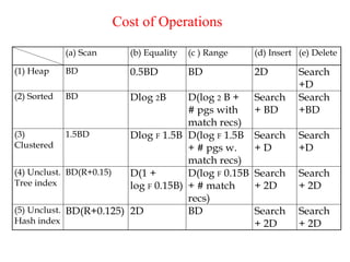
3. Compare the Heap file organization and Sequential file organization. [16]
4. What are the intuitions for tree indexes? and Explain about ISAM.
5. What are the causes of bucket overflow in a hash file organization? What
can be done to reduce the occurrence of bucket overflows?
6. Suppose that we are using extendable hashing on a file that contains
records with the following search-key values: 2,3,5,7,11,17,19,23,29,31
Show the extendable hash structure for this file if the hash function is
h(x) = x mod 8 and buckets can hold three records.
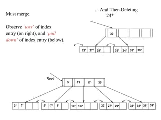
7. Explain about the B+tree file organization in detail..
8. When is it preferable to use a dense index rather than a sparse index?
Explain your answer.
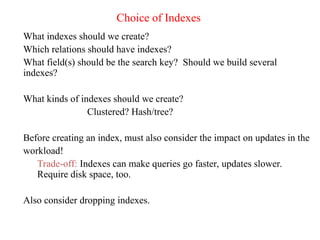
9. Since indices speed query processing, why might they not be kept on
several search keys? List as many reasons as possible.
10. Write briefly about Primary and secondary Indexes.