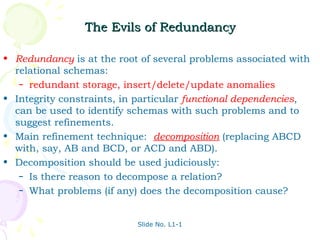
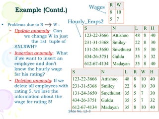
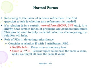
Steps in Database Design Process
ER Concepts (Entities, Attributes, Associations, etc)
ER Notations
Class Hierarchies
ER concepts, notations with appropriate examples. how to model databases using ER techniques.
In this part of the course, meta languages for describing grammars are introduced. Bottom-up and top-down parsers are derivation steps are described. Finally, ambiguous grammars are defined.
Christoph Koch is a professor of Computer Science at EPFL, specializing in data management. Until 2010, he was an Associate Professor in the Department of Computer Science at Cornell University. Previously to this, from 2005 to 2007, he was an Associate Professor of Computer Science at Saarland University. Earlier, he obtained his PhD in Artificial Intelligence from TU Vienna and CERN (2001), was a postdoctoral researcher at TU Vienna and the University of Edinburgh (2001-2003), and an assistant professor at TU Vienna (2003-2005). He has won Best Paper Awards at PODS 2002, ICALP 2005, and SIGMOD 2011, an Outrageous Ideas and Vision Paper Award at CIDR 2013, a Google Research Award (in 2009), and an ERC Grant (in 2011). He is a PI of the FET Flagship Human Brain Project and of NCCR MARVEL, a new Swiss national research center for materials research. He (co-)chaired the program committees of DBPL 2005, WebDB 2008, ICDE 2011, VLDB 2013, and was PC vice-chair of ICDE 2008 and ICDE 2009. He has served on the editorial board of ACM Transactions on Internet Technology and as Editor-in-Chief of PVLDB.
The presentation discusses about the following topics:
DBMS Architecture
Relational Algebra Review
Relational calculus
Relational calculus building blocks
Tuple relational calculus
Tuple relational calculus Formulas
With the raise of NoSQL databases consistency models that are less strict than ACID transactions became popular again. After the first enthusiasm the developer community became aware that those relaxed consistency models hold some new challenges they never knew about in the ACID world. Fortunately there are some concepts around how to deal with those challenges. This presentation gives a rough introduction into the different consistency models that are available and their characteristics. Then it focusses on two techniques to deal with relaxed consistency. The first one are quorum-based reads and writes which provides a client-side strong consistency model (even if the database only implements eventual consistency). Then CRDTs (Conflict-free Replicated Data Types) are presented. CRDTs are self-stabilizing data structures which are designed for environments with extremely high availability requirements - and thus extremely weak consistency guarantees. Even though as always the majority of the information is on the voice track, I designed the slides in a way that they also provide some useful information without the voice.
GridMate - End to end testing is a critical piece to ensure quality and avoid...ThomasParaiso2
End to end testing is a critical piece to ensure quality and avoid regressions. In this session, we share our journey building an E2E testing pipeline for GridMate components (LWC and Aura) using Cypress, JSForce, FakerJS…
Unlocking Productivity: Leveraging the Potential of Copilot in Microsoft 365, a presentation by Christoforos Vlachos, Senior Solutions Manager – Modern Workplace, Uni Systems
UiPath Test Automation using UiPath Test Suite series, part 5DianaGray10
Welcome to UiPath Test Automation using UiPath Test Suite series part 5. In this session, we will cover CI/CD with devops.
Topics covered:
CI/CD with in UiPath
End-to-end overview of CI/CD pipeline with Azure devops
Speaker:
Lyndsey Byblow, Test Suite Sales Engineer @ UiPath, Inc.
LF Energy Webinar: Electrical Grid Modelling and Simulation Through PowSyBl -...DanBrown980551
Do you want to learn how to model and simulate an electrical network from scratch in under an hour?
Then welcome to this PowSyBl workshop, hosted by Rte, the French Transmission System Operator (TSO)!
During the webinar, you will discover the PowSyBl ecosystem as well as handle and study an electrical network through an interactive Python notebook.
PowSyBl is an open source project hosted by LF Energy, which offers a comprehensive set of features for electrical grid modelling and simulation. Among other advanced features, PowSyBl provides:
- A fully editable and extendable library for grid component modelling;
- Visualization tools to display your network;
- Grid simulation tools, such as power flows, security analyses (with or without remedial actions) and sensitivity analyses;
The framework is mostly written in Java, with a Python binding so that Python developers can access PowSyBl functionalities as well.
What you will learn during the webinar:
- For beginners: discover PowSyBl's functionalities through a quick general presentation and the notebook, without needing any expert coding skills;
- For advanced developers: master the skills to efficiently apply PowSyBl functionalities to your real-world scenarios.
Smart TV Buyer Insights Survey 2024 by 91mobiles.pdf91mobiles
91mobiles recently conducted a Smart TV Buyer Insights Survey in which we asked over 3,000 respondents about the TV they own, aspects they look at on a new TV, and their TV buying preferences.
State of ICS and IoT Cyber Threat Landscape Report 2024 previewPrayukth K V
The IoT and OT threat landscape report has been prepared by the Threat Research Team at Sectrio using data from Sectrio, cyber threat intelligence farming facilities spread across over 85 cities around the world. In addition, Sectrio also runs AI-based advanced threat and payload engagement facilities that serve as sinks to attract and engage sophisticated threat actors, and newer malware including new variants and latent threats that are at an earlier stage of development.
The latest edition of the OT/ICS and IoT security Threat Landscape Report 2024 also covers:
State of global ICS asset and network exposure
Sectoral targets and attacks as well as the cost of ransom
Global APT activity, AI usage, actor and tactic profiles, and implications
Rise in volumes of AI-powered cyberattacks
Major cyber events in 2024
Malware and malicious payload trends
Cyberattack types and targets
Vulnerability exploit attempts on CVEs
Attacks on counties – USA
Expansion of bot farms – how, where, and why
In-depth analysis of the cyber threat landscape across North America, South America, Europe, APAC, and the Middle East
Why are attacks on smart factories rising?
Cyber risk predictions
Axis of attacks – Europe
Systemic attacks in the Middle East
Download the full report from here:
https://sectrio.com/resources/ot-threat-landscape-reports/sectrio-releases-ot-ics-and-iot-security-threat-landscape-report-2024/
Communications Mining Series - Zero to Hero - Session 1DianaGray10
This session provides introduction to UiPath Communication Mining, importance and platform overview. You will acquire a good understand of the phases in Communication Mining as we go over the platform with you. Topics covered:
• Communication Mining Overview
• Why is it important?
• How can it help today’s business and the benefits
• Phases in Communication Mining
• Demo on Platform overview
• Q/A
Observability Concepts EVERY Developer Should Know -- DeveloperWeek Europe.pdfPaige Cruz
Monitoring and observability aren’t traditionally found in software curriculums and many of us cobble this knowledge together from whatever vendor or ecosystem we were first introduced to and whatever is a part of your current company’s observability stack.
While the dev and ops silo continues to crumble….many organizations still relegate monitoring & observability as the purview of ops, infra and SRE teams. This is a mistake - achieving a highly observable system requires collaboration up and down the stack.
I, a former op, would like to extend an invitation to all application developers to join the observability party will share these foundational concepts to build on:
GraphRAG is All You need? LLM & Knowledge GraphGuy Korland
Guy Korland, CEO and Co-founder of FalkorDB, will review two articles on the integration of language models with knowledge graphs.
1. Unifying Large Language Models and Knowledge Graphs: A Roadmap.
https://arxiv.org/abs/2306.08302
2. Microsoft Research's GraphRAG paper and a review paper on various uses of knowledge graphs:
https://www.microsoft.com/en-us/research/blog/graphrag-unlocking-llm-discovery-on-narrative-private-data/
Pushing the limits of ePRTC: 100ns holdover for 100 daysAdtran
At WSTS 2024, Alon Stern explored the topic of parametric holdover and explained how recent research findings can be implemented in real-world PNT networks to achieve 100 nanoseconds of accuracy for up to 100 days.
The Art of the Pitch: WordPress Relationships and SalesLaura Byrne
Clients don’t know what they don’t know. What web solutions are right for them? How does WordPress come into the picture? How do you make sure you understand scope and timeline? What do you do if sometime changes?
All these questions and more will be explored as we talk about matching clients’ needs with what your agency offers without pulling teeth or pulling your hair out. Practical tips, and strategies for successful relationship building that leads to closing the deal.
SAP Sapphire 2024 - ASUG301 building better apps with SAP Fiori.pdfPeter Spielvogel
Building better applications for business users with SAP Fiori.
• What is SAP Fiori and why it matters to you
• How a better user experience drives measurable business benefits
• How to get started with SAP Fiori today
• How SAP Fiori elements accelerates application development
• How SAP Build Code includes SAP Fiori tools and other generative artificial intelligence capabilities
• How SAP Fiori paves the way for using AI in SAP apps
Why You Should Replace Windows 11 with Nitrux Linux 3.5.0 for enhanced perfor...SOFTTECHHUB
The choice of an operating system plays a pivotal role in shaping our computing experience. For decades, Microsoft's Windows has dominated the market, offering a familiar and widely adopted platform for personal and professional use. However, as technological advancements continue to push the boundaries of innovation, alternative operating systems have emerged, challenging the status quo and offering users a fresh perspective on computing.
One such alternative that has garnered significant attention and acclaim is Nitrux Linux 3.5.0, a sleek, powerful, and user-friendly Linux distribution that promises to redefine the way we interact with our devices. With its focus on performance, security, and customization, Nitrux Linux presents a compelling case for those seeking to break free from the constraints of proprietary software and embrace the freedom and flexibility of open-source computing.
GDG Cloud Southlake #33: Boule & Rebala: Effective AppSec in SDLC using Deplo...James Anderson
Effective Application Security in Software Delivery lifecycle using Deployment Firewall and DBOM
The modern software delivery process (or the CI/CD process) includes many tools, distributed teams, open-source code, and cloud platforms. Constant focus on speed to release software to market, along with the traditional slow and manual security checks has caused gaps in continuous security as an important piece in the software supply chain. Today organizations feel more susceptible to external and internal cyber threats due to the vast attack surface in their applications supply chain and the lack of end-to-end governance and risk management.
The software team must secure its software delivery process to avoid vulnerability and security breaches. This needs to be achieved with existing tool chains and without extensive rework of the delivery processes. This talk will present strategies and techniques for providing visibility into the true risk of the existing vulnerabilities, preventing the introduction of security issues in the software, resolving vulnerabilities in production environments quickly, and capturing the deployment bill of materials (DBOM).
Speakers:
Bob Boule
Robert Boule is a technology enthusiast with PASSION for technology and making things work along with a knack for helping others understand how things work. He comes with around 20 years of solution engineering experience in application security, software continuous delivery, and SaaS platforms. He is known for his dynamic presentations in CI/CD and application security integrated in software delivery lifecycle.
Gopinath Rebala
Gopinath Rebala is the CTO of OpsMx, where he has overall responsibility for the machine learning and data processing architectures for Secure Software Delivery. Gopi also has a strong connection with our customers, leading design and architecture for strategic implementations. Gopi is a frequent speaker and well-known leader in continuous delivery and integrating security into software delivery.
Elizabeth Buie - Older adults: Are we really designing for our future selves?
Unit 05 dbms
1. DATABASE MANAGEMENT SYSTEMS
MALLA REDDY ENGG. COLLEGE HYD
II B. Tech CSE II Semester
UNIT-V PPT SLIDES
Text Books: (1) DBMS by Raghu Ramakrishnan
(2) DBMS by Sudarshan and Korth
2. INDEX
UNIT-5 PPT SLIDES
S.NO Module as per Lecture PPT
Session planner No Slide NO
----------------------------------------------------------------------------------------------------------------------
1. Introduction to Schema Refinement L1 L1- 1 to L1- 7
2. Functional Dependencies L2 L2- 1 to L2- 10
3. Normal Forms L3 L3- 1 to L3- 9
4. Decompositions L4 L4- 1 to L4- 10
5. Schema refinement in database design L5 L5- 1 to L5- 4
6. Fourth Normal Form L6 L6- 1 to L6 -4
7. Fifth normal form L7 L7- 1 to L7- 3
3. The Evils of Redundancy
• Redundancy is at the root of several problems associated with
relational schemas:
– redundant storage, insert/delete/update anomalies
• Integrity constraints, in particular functional dependencies,
can be used to identify schemas with such problems and to
suggest refinements.
• Main refinement technique: decomposition (replacing ABCD
with, say, AB and BCD, or ACD and ABD).
• Decomposition should be used judiciously:
– Is there reason to decompose a relation?
– What problems (if any) does the decomposition cause?
Slide No. L1-1
4. INTRODUCTION TO SCHEMA REFINEMENT
Problems Caused by Redundancy
• Storing the same information redundantly, that is,
in more than one place within a database, can lead
to several problems:
• Redundant storage: Some information is stored
repeatedly.
• Update anomalies: If one copy of such repeated
data is updated, an inconsistency
• is created unless all copies are similarly updated.
• Insertion anomalies: It may not be possible to
store some information unless
• some other information is stored as well.
• Deletion anomalies: It may not be possible to
delete some information without
Slide No:L1-2
5. • losing some other information as well.
• Consider a relation obtained by translating a
variant of the Hourly Emps entity set
Ex: Hourly Emps(ssn, name, lot, rating, hourly
wages, hours worked)
• The key for Hourly Emps is ssn. In addition,
suppose that the hourly wages attribute
• is determined by the rating attribute. That is,
for a given rating value, there is only
• one permissible hourly wages value. This IC is
an example of a functional dependency.
• It leads to possible redundancy in the relation
Hourly Emps
Slide No:L1-3
6. Use of Decompositions
• Intuitively, redundancy arises when a relational
schema forces an association between attributes
that is not natural.
• Functional dependencies (ICs) can be used to
identify such situations and to suggest revetments
to the schema.
• The essential idea is that many problems arising
from redundancy can be addressed by replacing a
relation with a collection of smaller relations.
• Each of the smaller relations contains a subset of
the attributes of the original relation.
• We refer to this process as decomposition of the
larger relation into the smaller relations
Slide No:L1-4
7. • We can deal with the redundancy in Hourly Emps by
decomposing it into two relations:
• Hourly Emps2(ssn, name, lot, rating, hours worked)
• Wages(rating, hourly wages)
ratin hourlywages
g
8 10
5 7
Slide No:L1-5
9. Problems Related to Decomposition
• Unless we are careful, decomposing a relation
schema can create more problems than it solves.
• Two important questions must be asked
repeatedly:
• 1. Do we need to decompose a relation?
• 2. What problems (if any) does a given
decomposition cause?
• To help with the rst question, several normal forms
have been proposed for relations.
• If a relation schema is in one of these normal
forms, we know that certain kinds of
• problems cannot arise. Considering the n
Slide No:L1-7
10. Functional Dependencies (FDs)
• A functional dependency X Y→holds over relation R if, for
every allowable instance r of R:
– t1 ∈ r, t2 ∈ r, π X (t1) = π X (t2) implies π (t1) = π Y(t2)
Y
– i.e., given two tuples in r, if the X values agree, then the Y
values must also agree. (X and Y are sets of attributes.)
• An FD is a statement about all allowable relations.
– Must be identified based on semantics of application.
– Given some allowable instance r1 of R, we can check if it
violates some FD f, but we cannot tell if f holds over R!
• K is a candidate key for R means that K→ R
– However, K → R does not require K to be minimal!
Slide No. L2-1
11. Example: Constraints on Entity Set
• Consider relation obtained from Hourly_Emps:
– Hourly_Emps (ssn, name, lot, rating, hrly_wages,
hrs_worked)
• Notation: We will denote this relation schema by listing the
attributes: SNLRWH
– This is really the set of attributes {S,N,L,R,W,H}.
– Sometimes, we will refer to all attributes of a relation by
using the relation name. (e.g., Hourly_Emps for SNLRWH)
• Some FDs on Hourly_Emps:
– ssn is the key: S → SNLRWH
– rating determines hrly_wages: R→ W
Slide No. L2-2
12. Wages R W
Example (Contd.) 8 10
5 7
Hourly_Emps2
• Problems due to R →W: S N L R H
– Update anomaly: Can
we change W in just 123-22-3666 Attishoo 48 8 40
the 1st tuple of 231-31-5368 Smiley 22 8 30
SNLRWH?
131-24-3650 Smethurst 35 5 30
– Insertion anomaly: What
if we want to insert an 434-26-3751 Guldu 35 5 32
employee and don’t 612-67-4134 Madayan 35 8 40
know the hourly wage
S N L R W H
for his rating?
– Deletion anomaly: If we 123-22-3666 Attishoo 48 8 10 40
delete all employees with 231-31-5368 Smiley 22 8 10 30
rating 5, we lose the 131-24-3650 Smethurst 35 5 7 30
information about the
wage for rating 5! 434-26-3751 Guldu 35 5 7 32
612-67-4134 Madayan 35 8 10 40
Slide No. L2-3
13. Constraints on a Relationship Set
• Suppose that we have entity sets Parts, Suppliers,
and Departments, as well as a relationship set
Contracts that involves all of them. We refer to the
schema for Contracts as CQPSD. A contract with
contract id
• C species that a supplier S will supply some quantity
Q of a part P to a department D.
• We might have a policy that a department purchases
at most one part from any given supplier.
• Thus, if there are several contracts between the same
supplier and department,
• we know that the same part must be involved in all of
them. This constraint is an FD, DS ! P.
Slide No:L2-4
14. Reasoning About FDs
• Given some FDs, we can usually infer additional FDs:
– ssn → did, did→ lot implies ssn → lot
• An FD f is implied by a set of FDs F if f holds whenever all
FDs in F hold.
– = closure of F is the set of all FDs that are implied by F.
F+
• Armstrong’s Axioms (X, Y, Z are sets of attributes):
– Reflexivity: If X ⊆ Y, then Y → X
– Augmentation: If X → Y, then XZ → YZ for any Z
– Transitivity: If X → Y and Y → Z, then X → Z
• These are sound and complete inference rules for FDs!
Slide No. L2-5
15. Reasoning About FDs (Contd.)
• Couple of additional rules (that follow from AA):
– Union: If X → Y and X → Z, then X → YZ
– Decomposition: If X → YZ, then X → Y and X →
Z
→
• Example: Contracts(cid,sid,jid,did,pid,qty,value), and:
– C is the key: C CSJDPQV
→
– Project purchases each part using single contract:
– JP C
→
– Dept purchases at most one part from a supplier: S
→
– D P → →
• JP → C, C →
CSJDPQV imply JP CSJDPQV
• SD → implies→SDJ
P JP →
• SDJ JP, JP CSJDPQV imply SDJ CSJDPQV
Slide No. L2-6
16. Reasoning About FDs (Contd.)
• Computing the closure of a set of FDs can be expensive. (Size
of closure is exponential in # attrs!)
• Typically, we just want to check if a given FD X →Y is in the
closure of a set of FDs F. An efficient check:
– Compute attribute closure of X (denoted X
+
) wrt F:
• Set of all attributes A such that X → A is in F +
• There is a linear time algorithm to compute this.
– Check if Y is in X +
• Does F = {A → B, B→ C, C D → E } imply A → E?
– i.e, is A → E in the closure F + ? Equivalently, is E in +
A
?
Slide No. L2-7
17. Closure of a Set of FDs
• The set of all FDs implied by a given set F of FDs is
called the closure of F and is denoted as F+.
• An important question is how we can infer, or
compute, the closure of a given set F of FDs.
• The following three rules, called Armstrong's
Axioms, can be applied repeatedly to infer all FDs
implied by a set F of FDs.
• We use X, Y, and Z to denote sets of attributes over
a relation schema R:
Slide No:L2-8
18. Closure of a Set of FDs
• Reflexivity: If X Y, then X !Y.
• Augmentation: If X ! Y, then XZ ! YZ for any Z.
• Transitivity: If X ! Y and Y ! Z, then X ! Z.
• Armstrong's Axioms are sound in that they generate
only FDs in F+ when applied to a set F of FDs.
• They are complete in that repeated application of
these rules will generate all FDs in the closure F+.
• It is convenient to use some additional rules while
reasoning about F+:
• Union: If X ! Y and X ! Z, then X !YZ.
• Decomposition: If X ! YZ, then X !Y and X ! Z.
• These additional rules are not essential; their
soundness can be proved using Armstrong's Axioms.
Slide No:L2-9
19. Attribute Closure
• If we just want to check whether a given dependency,
say, X → Y, is in the closure of a set F of FDs,
• we can do so eciently without computing F+. We rst
compute the attribute closure X+ with respect to F,
• which is the set of attributes A such that X → A can be
inferred using the Armstrong Axioms.
• The algorithm for computing the attribute closure of a
set X of attributes is
• closure = X;
repeat until there is no change: {
if there is an FD U → V in F such that U subset of
closure,
then set closure = closure union of V
}
Slide No:L2-10
20. NORMAL FORMS
• The normal forms based on FDs are rst normal form (1NF),
second normal form (2NF), third normal form (3NF), and
Boyce-Codd normal form (BCNF).
• These forms have increasingly restrictive requirements:
Every relation in BCNF is also in 3NF,
• every relation in 3NF is also in 2NF, and every relation in
2NF is in 1NF.
• A relation
• is in first normal form if every field contains only atomic
values, that is, not lists or sets.
• This requirement is implicit in our defition of the relational
model.
• Although some of the newer database systems are
relaxing this requirement
• 2NF is mainly of historical interest.
• 3NF and BCNF are important from a database design
standpoint.
Slide No:L3-1
21. Normal Forms
• Returning to the issue of schema refinement, the first
question to ask is whether any refinement is needed!
• If a relation is in a certain normal form (BCNF, 3NF etc.), it is
known that certain kinds of problems are avoided/minimized.
This can be used to help us decide whether decomposing the
relation will help.
• Role of FDs in detecting redundancy:
– Consider a relation R with 3 attributes, ABC.
• No FDs hold: There is no redundancy here.
• Given A → B: Several tuples could have the same A value,
and if so, they’ll all have the same B value!
Slide No. L3-2
22. First Normal Form
1NF (First Normal Form)
• a relation R is in 1NF if and only if it has only single-
valued attributes (atomic values)
• EMP_PROJ (SSN, PNO, HOURS, ENAME, PNAME,
PLOCATION)
PLOCATION is not in 1NF (multi-valued attrib.)
• solution: decompose the relation
EMP_PROJ2 (SSN, PNO, HOURS, ENAME, PNAME)
LOC (PNO, PLOCATION)
Slide No. L3-3
23. Second Normal Form
2NF (Second Normal Form)
• a relation R in 2NF if and only if it is in 1NF and
every nonkey column depends on a key not a subset
of a key
• all nonprime attributes of R must be fully
functionally dependent on a whole key(s) of the
relation, not a part of the key
• no violation: single-attribute key or no nonprime
attribute
Slide No. L3-4
24. Second Normal Form ( Contd)
2NF (Second Normal Form)
• violation: part of a key → nonkey
EMP_PROJ2 (SSN, PNO, HOURS, ENAME, PNAME)
SSN → ENAME
PNO → PNAME
• solution: decompose the relation
EMP_PROJ3 (SSN, PNO, HOURS)
EMP (SSN, ENAME)
PROJ (PNO, PNAME)
Slide No. L3-5
25. Third Normal Form
3NF (Third Normal Form)
• a relation R in 3NF if and only if it is in 2NF and
every nonkey column does not depend on another
nonkey column
• all nonprime attributes of R must be non-
transitively functionally dependent on a key of the
relation
• violation: nonkey → nonkey
• fig14.10: 2NF & 3NF normalization
Slide No. L3-6
26. Third Normal Form (Contd)
3NF (Third Normal Form)
• SUPPLIER (SNAME, STREET, CITY, STATE, TAX)
SNAME → STREET, CITY, STATE
STATE → TAX (nonkey → nonkey)
SNAME → STATE → TAX (transitive FD)
• solution: decompose the relation
SUPPLIER2 (SNAME, STREET, CITY, STATE)
TAXINFO (STATE, TAX)
Slide No. L3-7
27. Boyce-Codd Normal Form (BCNF)
• Reln R with FDs F is in BCNF if, for all X A →
in F+
– A
∈ X (called a trivial FD), or
– X contains a key for R.
• In other words, R is in BCNF if the only non-trivial FDs that
hold over R are key constraints.
– No dependency in R that can be predicted using FDs alone.
– If we are shown two tuples that agree upon
the X value, we cannot infer the A value in
one tuple from the A value in theX Y A
other.
– If example relation is in BCNF, the 2 tuples
x y1 a
must be identical (since X is a key).
x y2 ?
Slide No. L3-8
28. Third Normal Form (3NF)
• Reln R with FDs F is in 3NF if, for all X A→ in F+
– A
∈ X (called a trivial FD), or
– X contains a key for R, or
– A is part of some key for R.
• Minimality of a key is crucial in third condition above!
• If R is in BCNF, obviously in 3NF.
• If R is in 3NF, some redundancy is possible. It is a
compromise, used when BCNF not achievable (e.g., no ``good’’
decomp, or performance considerations).
– Lossless-join, dependency-preserving decomposition of R into
a collection of 3NF relations always possible.
Slide No. L3-9
29. Decomposition of a Relation Scheme
• Suppose that relation R contains attributes A1 ... An. A
decomposition of R consists of replacing R by two or more
relations such that:
– Each new relation scheme contains a subset of the
attributes of R (and no attributes that do not appear in R),
and
– Every attribute of R appears as an attribute of one of the
new relations.
• Intuitively, decomposing R means we will store instances of
the relation schemes produced by the decomposition, instead
of instances of R.
• E.g., Can decompose SNLRWH into SNLRH and RW.
Slide No. L4-1
30. Example Decomposition
• Decompositions should be used only when needed.
– SNLRWH has FDs S → SNLRWH and R→ W
– Second FD causes violation of 3NF; W values repeatedly
associated with R values. Easiest way to fix this is to
create a relation RW to store these associations, and to
remove W from the main schema:
• i.e., we decompose SNLRWH into SNLRH and RW
• The information to be stored consists of SNLRWH tuples. If
we just store the projections of these tuples onto SNLRH and
RW, are there any potential problems that we should be aware
of?
Slide No. L4-2
31. Problems with Decompositions
• There are three potential problems to consider:
– Some queries become more expensive.
• e.g., How much did sailor Joe earn? (salary = W*H)
– Given instances of the decomposed relations, we may not
be able to reconstruct the corresponding instance of the
original relation!
• Fortunately, not in the SNLRWH example.
– Checking some dependencies may require joining the
instances of the decomposed relations.
• Fortunately, not in the SNLRWH example.
• Tradeoff: Must consider these issues vs. redundancy.
Slide No. L4-3
32. Lossless Join Decompositions
• Decomposition of R into X and Y is lossless-join w.r.t. a set of
FDs F if, for every instance r that satisfies F:
– (r) (r) = r
π X πY
• It is always true that r (r) (r)
⊆ π π
– In general, the other direction X does hold! If it does, the
not Y
decomposition is lossless-join.
• Definition extended to decomposition into 3 or more relations
in a straightforward way.
• It is essential that all decompositions used to deal with
redundancy be lossless! (Avoids Problem (2).)
Slide No. L4-4
33. More on Lossless Join A B
1 2
A B C 4 5
• The decomposition of R into X and
7 2
Y is lossless-join wrt F if and only 1 2 3
if the closure of F contains: 4 5 6
B C
– X Y X, or 7 2 8
2 3
–X Y Y
∩ →
• In particular, the decomposition of
5 6
R into∩ →
UV and R - V is A B C
2 8
lossless-join if U V holds
over R.
1 2 3
4 5 6
7 2 8
→ 1 2 8
Slide No. L4-5 7 2 3
34. Dependency Preserving Decomposition
• Consider CSJDPQV, C is key, JP →
C and SD P.→
– BCNF decomposition: CSJDQV and SDP
– Problem: Checking JP
→ C requires a join!
• Dependency preserving decomposition (Intuitive):
– If R is decomposed into X, Y and Z, and we enforce the
FDs that hold on X, on Y and on Z, then all FDs that were
given to hold on R must also hold. (Avoids Problem (3).)
• Projection of set of FDs F: If R is decomposed into X, ...
projection of F onto X (denoted FX ) is the set of FDs U V
in F+ (closure of F ) such that U, V are in X.
→
Slide No. L4-6
35. Dependency Preserving Decompositions
(Contd.)
• Decomposition of R into X and Y is dependency preserving if
(FX union FY ) + = F +
– i.e., if we consider only dependencies in the closure F + that
can be checked in X without considering Y, and in Y
without considering X, these imply all dependencies in F +.
• Important to consider F +, not F, in this definition:
– ABC, A B, B C, C A, decomposed into AB and
BC. → → →
– Is this dependency preserving? Is C → A preserved?????
• Dependency preserving does not imply lossless join:
– ABC, A
→ B, decomposed into AB and BC.
• And vice-versa! (Example?)
Slide No. L4-7
36. Decomposition into BCNF
• Consider relation R with FDs F. If X Y→violates BCNF,
decompose R into R - Y and XY.
– Repeated application of this idea will give us a collection of
relations that are in BCNF; lossless join decomposition,
and guaranteed to terminate.
– e.g., CSJDPQV, key C, JP C, SD P, J S
– To deal with SD
→ → →
P, decompose into SDP, CSJDQV.
– To deal with J →S, decompose CSJDQV into JS and
CJDQV →
• In general, several dependencies may cause violation of BCNF.
The order in which we ``deal with’’ them could lead to very
different sets of relations!
Slide No. L4-8
37. BCNF and Dependency Preservation
• In general, there may not be a dependency preserving
decomposition into BCNF.
– e.g., CSZ, CS
→ Z, Z → C
– Can’t decompose while preserving 1st FD; not in BCNF.
• Similarly, decomposition of CSJDQV into SDP, JS and
CJDQV is not dependency preserving (w.r.t. the FDs JP
C, SD P and J S).
→ → →
– However, it is a lossless join decomposition.
– In this case, adding JPC to the collection of relations
gives us a dependency preserving decomposition.
• JPC tuples stored only for checking FD! (Redundancy!)
Slide No. L4-9
38. Decomposition into 3NF
• Obviously, the algorithm for lossless join decomp into BCNF
can be used to obtain a lossless join decomp into 3NF
(typically, can stop earlier).
• To ensure dependency preservation, one idea:
– If X Y is not preserved, add relation XY.
→
– Problem is that XY may violate 3NF! e.g., consider the
addition of CJP to `preserve’ JP C. What if we also
have J C? →
→
• Refinement: Instead of the given set of FDs F, use a minimal
cover for F.
Slide No. L4-10
39. SCHEMA REFINEMENT
Constraints on an Entity Set
• Consider the Hourly Emps relation again. The
constraint that attribute ssn is a key can be
expressed as an FD:
• { ssn }-> { ssn, name, lot, rating, hourly wages, hours
worked}
• For brevity, we will write this FD as S -> SNLRWH,
using a single letter to denote each attribute
• In addition, the constraint that the hourly wages
attribute is determined by the rating attribute is an
FD: R -> W.
Slide No:L5-1
40. Constraints on a Relationship Set
• The previous example illustrated how FDs can
help to rene the subjective decisions made
during ER design,
• but one could argue that the best possible ER
diagram would have led to the same nal set of
relations.
• Our next example shows how FD information
can lead to a set of relations that eliminates
some redundancy problems and is unlikely to
be arrived at solely through ER design.
Slide No:L5-2
41. Identifying Attributes of Entities
• in particular, it shows that attributes can easily be
associated with the `wrong' entity set during ER design.
• The ER diagram shows a relationship set called Works
In that is similar to the Works In relationship set
• Using the key constraint, we can translate this ER
diagram into two relations:
• Workers(ssn, name, lot, did, since)
Slide No:L5-3
42. Identifying Entity Sets
• Let Reserves contain attributes S, B, and D as before,
indicating that sailor S has a reservation for boat B
on day D.
• In addition, let there be an attribute C denoting the
credit card to which the reservation is charged.
• Suppose that every sailor uses a unique credit card
for reservations. This constraint is expressed by the
FD
S -> C. This constraint indicates that in relation
Reserves, we store the credit card number for a sailor
as often as we have reservations for that
• sailor, and we have redundancy and potential update
anomalies.
Slide No:L5-4
43. Multivalued Dependencies
• Suppose that we have a relation with attributes course,
teacher, and book, which we denote as CTB.
• The meaning of a tuple is that teacher T can teach
course C, and book B is a recommended text for the
course.
• There are no FDs; the key is CTB. However, the
recommended texts for a course are independent of the
instructor.
Slide No:L6-1
44. There are three points to note here:
• The relation schema CTB is in BCNF; thus we
would not consider decomposing it further if we
looked only at the FDs that hold over CTB.
• There is redundancy. The fact that Green can
teach Physics101 is recorded once per
recommended text for the course. Similarly, the
fact that Optics is a text for Physics101 is recorded
once per potential teacher.
• The redundancy can be eliminated by decomposing
CTB into CT and CB.
• Let R be a relation schema and let X and Y be
subsets of the attributes of R. Intuitively,
• the multivalued dependency X !! Y is said to hold
over R if, in every legal
Slide No:L6-2
45. • The redundancy in this example is due to the
constraint that the texts for a course are
independent of the instructors, which cannot
be epressed in terms of FDs.
• This constraint is an example of a multivalued
dependency, or MVD. Ideally, we should model
this situation using two binary relationship
sets, Instructors with attributes CT and Text
with attributes CB.
• Because these are two essentially independent
relationships, modeling them with a single
ternary relationship set with attributes CTB is
inappropriate.
Slide No:L6-3
46. • Three of the additional rules involve only MVDs:
• MVD Complementation: If X →→Y, then X →→ R −
XY
• MVD Augmentation: If X →→ Y and W > Z, then
WX →→ YZ.
• MVD Transitivity: If X →→ Y and Y →→ Z, then
X →→ (Z − Y ).
• Fourth Normal Form
• R is said to be in fourth normal form (4NF) if for
every MVD X →→Y that holds over R, one of the
following statements is true:
• Y subset of X or XY = R, or
• X is a superkey.
Slide No:L6-4
47. Join Dependencies
• A join dependency is a further generalization of
MVDs. A join dependency (JD) ∞{ R1,….. Rn } is
said to hold over a relation R if R1,…. Rn is a
lossless-join decomposition of R.
• An MVD X ->-> Y over a relation R can be expressed
as the join dependency ∞ { XY,X(R−Y)}
• As an example, in the CTB relation, the MVD C ->-
>T can be expressed as the join dependency ∞{ CT,
CB}
• Unlike FDs and MVDs, there is no set of sound and
complete inference rules for JDs.
Slide No:L7-1
48. Fifth Normal Form
• A relation schema R is said to be in fth normal
form (5NF) if for every JD ∞{ R1,…. Rn } that holds
over R, one of the following statements is true:
• Ri = R for some i, or
• The JD is implied by the set of those FDs over R in
which the left side is a key for R.
• The following result, also due to Date and Fagin,
identies conditions|again, detected using only FD
information|under which we can safely ignore JD
information.
• If a relation schema is in 3NF and each of its keys
consists of a single attribute,it is also in 5NF.
Slide No:L7-2
49. Inclusion Dependencies
• MVDs and JDs can be used to guide database
design, as we have seen, although they are less
common than FDs and harder to recognize and
reason about.
• In contrast, inclusion dependencies are very
intuitive and quite common. However, they
typically have little influence on database design
• The main point to bear in mind is that we should
not split groups of attributes that participate in an
inclusion dependency.
• Most inclusion dependencies in practice are key-
based, that is, involve only keys.
Slide No:L7-3