Deep Learning Convolutional Neural Network Densely Connected Huang, Liu, van der Maaten, Weinberger Machine Learning

1. Densely Connected Convolutional
Networks
Authors: Gao Huang*, Zhuang Liu*, Laurens van der Maaten,
Kilian Q. Weinberger
Presented by:
Arun Kumar (ENG18CS0047)
Ananth Desai (ENG18CS0034)
Evans Nikith Royan (ENG18CS0054)

2. CNN
Convolutional neural networks (CNNs) have
become the dominant machine learning
approach for visual object recognition.

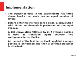
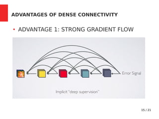
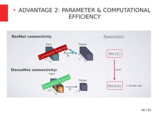
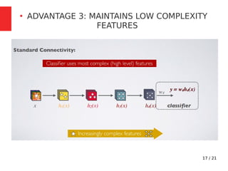
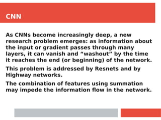
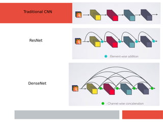
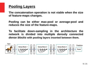
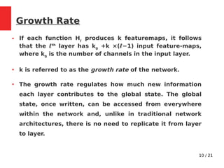
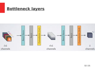
3. CNN
As CNNs become increasingly deep, a new
research problem emerges: as information about
the input or gradient passes through many
layers, it can vanish and “washout” by the time
it reaches the end (or beginning) of the network.
This problem is addressed by Resnets and by
Highway networks.
The combination of features using summation
may impede the information flow in the network.

4. ResNet
DenseNet
Traditional CNN

5. Resnet, Stochastic Depth, Densenet
Applications of Resnet: image recognition, localization,
and object detection
Stochastic depth: Better training of Resnet by dropping
layers randomly during training.
There is a great amount of redundancy in deep
(residual) networks.
There are direct connections from any layer to all
subsequent layers in Densenet.
A traditional CNN with L layers contains L connections. A
densenet with L layers contains L*(L+1)/2 connections.

6. Formula for Output at Each Layer
Consider a single image x0 that is passed through a CNN.
The network comprises L layers, each of which implements
a non-linear transformation Hℓ(·), where ℓ indexes the layer.
Hℓ(·) can contain operations such as BN, ReLU, Pool and
Conv.
In traditional CNN,
In Resnet,
In Densenet,

7. Hℓ(·) is a Composite Function

8. DenseNets
DenseNet layers are very narrow (eg: 12 filters
per layer), adding only a small set of feature-
maps to the “collective knowledge” of the
network and keep the remaining feature-maps
unchanged; the final classifier makes a decision
based on all feature-maps in the network.
DenseNets exploit the potential of the network
through feature reuse.
Inception networks also concatenate features
from different layers.

9. 9 / 21
Pooling Layers
The concatenation operation is not viable when the size
of feature-maps changes.
Pooling can be either max-pool or average-pool and
reduces the size of the feature-maps.
To facilitate down-sampling in the architecture the
network is divided into multiple densely connected
dense blocks with pooling layers inserted between them.

10. 10 / 21
Growth Rate
● If each function Hℓ
produces k featuremaps, it follows
that the ℓth
layer has k0
+k ×(ℓ−1) input feature-maps,
where k0
is the number of channels in the input layer.
●
k is referred to as the growth rate of the network.
●
The growth rate regulates how much new information
each layer contributes to the global state. The global
state, once written, can be accessed from everywhere
within the network and, unlike in traditional network
architectures, there is no need to replicate it from layer
to layer.

11. 11 / 21
Bottleneck layers
●
Although each layer only produces k output
feature-maps, it typically has many more inputs.
●
A 1×1 convolution can be introduced as bottleneck
layer before each 3×3 convolution to reduce the
number of input feature-maps, and thus to improve
computational efficiency.

12. 12 / 21
Bottleneck layers

13. 13 / 21
Compression
●
To further improve model compactness, the number
of feature-maps is reduced at transition layers.
●
If a dense block contains m feature-maps, we let
the following transition layer generate [θm] output
feature maps, where 0 < θ ≤1 is referred to as the
compression factor.

14. 14 / 21
Implementation
●
The DenseNet used in the experiments has three
dense blocks that each has an equal number of
layers.
●
Before entering the first dense block, a convolution
with 16 output channels is performed on the input
images.
●
A 1×1 convolution followed by 2×2 average pooling
is used as transition layers between two
contiguous dense blocks.
●
At the end of the last dense block, a global average
pooling is performed and then a softmax classifier
is attached.

15. 15 / 21
ADVANTAGES OF DENSE CONNECTIVITY
●
ADVANTAGE 1: STRONG GRADIENT FLOW

16. 16 / 21
●
ADVANTAGE 2: PARAMETER & COMPUTATIONAL
EFFICIENCY

17. 17 / 21
●
ADVANTAGE 3: MAINTAINS LOW COMPLEXITY
FEATURES

18. 18 / 21

19. 19 / 21
RESULTS
●
Results on CIFAR-10:

20. 20 / 21
●
Results on CIFAR-100:

21. 21 / 21
●
Results on IMAGENET