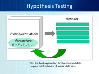
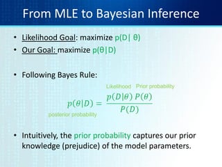
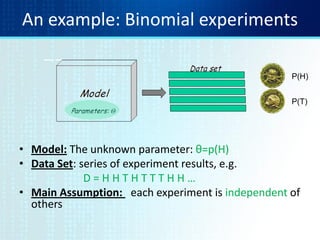
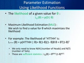
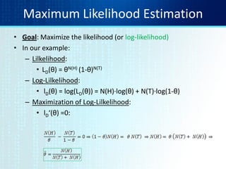
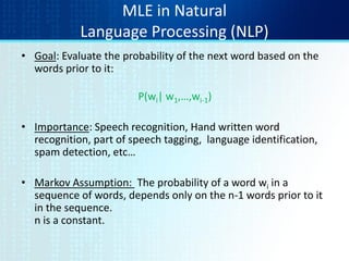
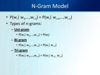
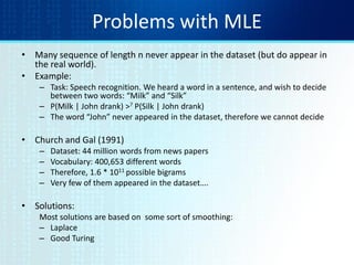
1. Hypothesis testing and maximum likelihood estimation (MLE) are introduced as methods for finding the best explanation for observed data and predicting similar data. 2. MLE aims to find the parameter value that maximizes the likelihood function, which represents the probability of the data given different parameter values. 3. For language models, MLE is used to estimate the probability of the next word given previous words by calculating n-gram probabilities from word co-occurrence counts in training data.

1. Hypothesis testing, MLE, language models
Kira Radinsky
Based on some slides of Ilan Gronau,
Ydo Wexler, Dan Geiger & Nir Fridman

2. Hypothesis Testing
•Find the best explanation for the observed data
•Helps predict behavior of similar data sets

3. An example: Binomial experiments
• Model: The unknown parameter: θ=p(H)
• Data Set: series of experiment results, e.g.
D = H H T H T T T H H …
• Main Assumption: each experiment is independent of
others
P(H)
P(T)

4. Parameter Estimation
Using Likelihood Functions
• The likelihood of a given value for θ :
LD (θ) = p(D| θ)
• Maximum Likelihood Estimation (MLE) :
We wish to find a value for θ which maximizes the
likelihood
• For example: The likelihood of ‘HTTHH’ is:
LHTTHH (θ) = p(HTTHH | θ)= θ(1-θ)(1- θ)θ θ = θ3(1-θ)2
• We only need to know N(H) (number of Heads) and N(T)
(number of Tails).
• These are sufficient statistics : LD(θ) = θN(H) (1-θ)N(T)

5. Sufficient Statistics
• A sufficient statistic is a function of the data
that summarizes the relevant information for
the likelihood.
• s(D) is a sufficient statistics if for any two
datasets D and D’:
s(D) = s(D’ ) => LD(θ) = LD’(θ)
• Likelihood may be calculated on the statistics.

6. Maximum Likelihood Estimation
• Goal: Maximize the likelihood (or log-likelihood)
• In our example:
– Lilkelihood:
• LD(θ) = θN(H) (1-θ)N(T)
– Log-Lilkelihood:
• lD(θ) = log(LD(θ)) = N(H)·log(θ) + N(T)·log(1-θ)
– Maximization of Log-Lilkelihood:
• lD‘(θ) =0:

7. MLE with multiple parameters
• What if we have several parameters θ1, θ2,…, θK that we
wish to learn?
• Examples:
– die toss (K=6)
– Grades (K=100)
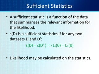
• Sufficient statistics [assumption: a series of independent experiments]:
– N1, N2, …, NK - the number of times each outcome was observed
• Likelihood:
• MLE:

8. From MLE to Bayesian Inference
• Likelihood Goal: maximize p(D| θ)
• Our Goal: maximize p(θ|D)
• Following Bayes Rule:
• Intuitively, the prior probability captures our prior
knowledge (prejudice) of the model parameters.
posterior probability
Likelihood Prior probability

9. MLE in Natural
Language Processing (NLP)
• Goal: Evaluate the probability of the next word based on the
words prior to it:
P(wi| w1,…,wi-1)
• Importance: Speech recognition, Hand written word
recognition, part of speech tagging, language identification,
spam detection, etc…
• Markov Assumption: The probability of a word wi in a
sequence of words, depends only on the n-1 words prior to it
in the sequence.
n is a constant.

10. N-Gram Model
• P(wi| w1,…,wi-1) = P(wi| wi-n,…,wi-1)
• Types of n-grams:
– Uni-gram
• P(wi| w1,…,wi-1) = P(wi)
– Bi-gram
• P(wi| w1,…,wi-1) = P(wi| wi-1)
– Tri-gram
• P(wi| w1,…,wi-1) = P(wi| wi-2 , wi-1)

11. MLE in NLP
• Problem:
How do we evaluate P(wi) , P(wi| wi-1) , P(wi| wi-2 , wi-1) ?
• Proposal: MLE

12. Problems with MLE
• Many sequence of length n never appear in the dataset (but do appear in
the real world).
• Example:
– Task: Speech recognition. We heard a word in a sentence, and wish to decide
between two words: “Milk” and “Silk”
– P(Milk | John drank) >? P(Silk | John drank)
– The word “John” never appeared in the dataset, therefore we cannot decide
• Church and Gal (1991)
– Dataset: 44 million words from news papers
– Vocabulary: 400,653 different words
– Therefore, 1.6 * 1011 possible bigrams
– Very few of them appeared in the dataset….
• Solutions:
Most solutions are based on some sort of smoothing:
– Laplace
– Good Turing

13. Evaluation
• The null hypothesis, denoted by H0
• The alternative hypothesis, denoted by H1.
• Should we reject the null hypothesis in favor of the alternative?
Input:
– a value from a certain distribution
– we don't know what the parameter of that distribution is.
Test:
– How likely it is that the value we were given could have come from the
distribution with this predicted parameter?
– If it's not very likely, we reject the null hypothesis in favor of the alternative.
• Critical Region
– But what exactly is "not very likely"?
– We choose a region known as the critical region. If the result of our
test lies in this region, then we reject the null hypothesis in favor of
the alternative.

14. Empirical Evolution methods
• Divide to train and test
– Leave one out
• Cross validation
– 10 fold cross validation
– 5x2 cross validation
• Never (never never!) perform evaluation on
the training data
Never!