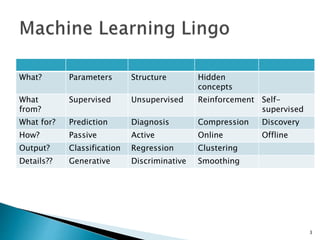
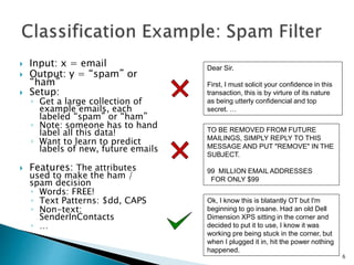
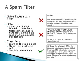
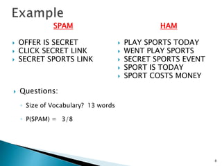
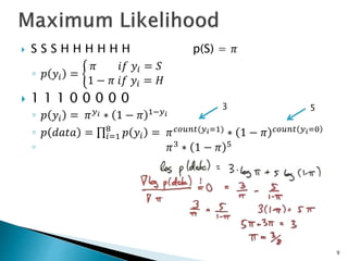
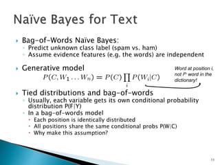
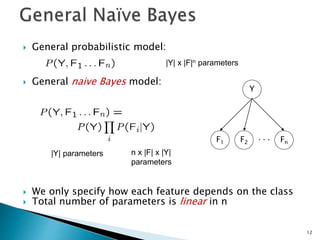
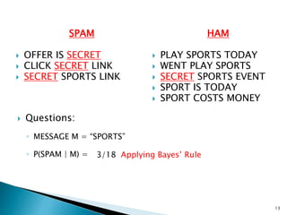
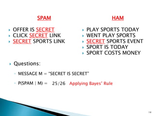
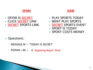
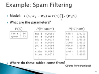
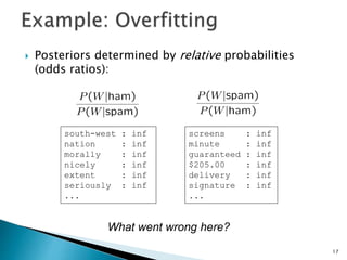
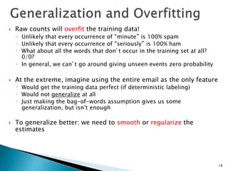
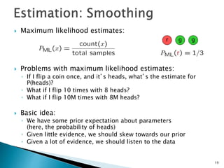
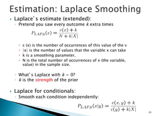
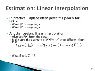
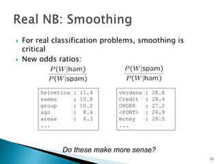
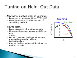
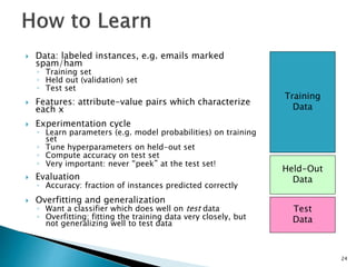
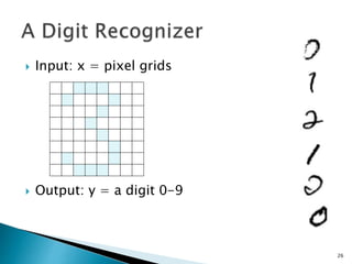
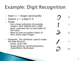
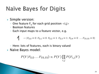
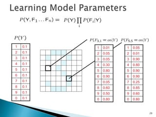
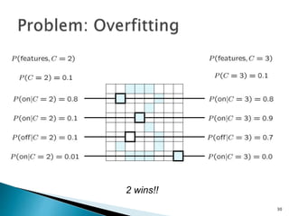
Supervised learning: Types of Machine Learning

Made by: Maor Levy, Temple University 2012 1

 Up until now: how to reason in a give model
 Machine learning: how to acquire a model on
the basis of data / experience
◦ Learning parameters (e.g. probabilities)
◦ Learning structure (e.g. BN graphs)
◦ Learning hidden concepts (e.g. clustering)
2

What? Parameters Structure Hidden
concepts
What
from?
Supervised Unsupervised Reinforcement Self-
supervised
What for? Prediction Diagnosis Compression Discovery
How? Passive Active Online Offline
Output? Classification Regression Clustering
Details?? Generative Discriminative Smoothing
3

4
 Commonly attributed to William of Ockham
(1290-1349). This was formulated about
fifteen hundred years after Epicurus.
◦ In sharp contrast to the principle of multiple
explanations, it states: Entities should not be
multiplied beyond necessity.
 Commonly explained as: when have choices,
choose the simplest theory.
 Bertrand Russell: “It is vain to do with more
what can be done with fewer.”

(c)
(a) (b) (d)
x x x x
f(x) f(x) f(x) f(x)
Given a training set:
(x1, y1), (x2, y2), (x3, y3), … (xn, yn)
Where each yi was generated by an unknown y = f (x),
Discover a function h that approximates the true function f.
5

 Input: x = email
 Output: y = “spam” or
“ham”
 Setup:
◦ Get a large collection of
example emails, each
labeled “spam” or “ham”
◦ Note: someone has to hand
label all this data!
◦ Want to learn to predict
labels of new, future emails
 Features: The attributes
used to make the ham /
spam decision
◦ Words: FREE!
◦ Text Patterns: $dd, CAPS
◦ Non-text:
SenderInContacts
◦ …
Dear Sir.
First, I must solicit your confidence in this
transaction, this is by virture of its nature
as being utterly confidencial and top
secret. …
TO BE REMOVED FROM FUTURE
MAILINGS, SIMPLY REPLY TO THIS
MESSAGE AND PUT "REMOVE" IN THE
SUBJECT.
99 MILLION EMAIL ADDRESSES
FOR ONLY $99
Ok, I know this is blatantly OT but I'm
beginning to go insane. Had an old Dell
Dimension XPS sitting in the corner and
decided to put it to use, I know it was
working pre being stuck in the corner, but
when I plugged it in, hit the power nothing
happened.
6

 Naïve Bayes spam
filter
 Data:
◦ Collection of emails,
labeled spam or ham
◦ Note: someone has to
hand label all this data!
◦ Split into training, held-
out, test sets
 Classifiers
◦ Learn on the training set
◦ (Tune it on a held-out
set)
◦ Test it on new emails
Dear Sir.
First, I must solicit your confidence in this
transaction, this is by virture of its nature
as being utterly confidencial and top
secret. …
TO BE REMOVED FROM FUTURE
MAILINGS, SIMPLY REPLY TO THIS
MESSAGE AND PUT "REMOVE" IN THE
SUBJECT.
99 MILLION EMAIL ADDRESSES
FOR ONLY $99
Ok, Iknow this is blatantly OT but I'm
beginning to go insane. Had an old Dell
Dimension XPS sitting in the corner and
decided to put it to use, I know it was
working pre being stuck in the corner, but
when I plugged it in, hit the power nothing
happened.
7

SPAM
 OFFER IS SECRET
 CLICK SECRET LINK
 SECRET SPORTS LINK
8
HAM
 PLAY SPORTS TODAY
 WENT PLAY SPORTS
 SECRET SPORTS EVENT
 SPORT IS TODAY
 SPORT COSTS MONEY
 Questions:
◦ Size of Vocabulary?
◦ P(SPAM) =
13 words
3/8

9
 S S S H H H H H H p(S) = 𝜋
◦ 𝑝 𝑦𝑖 =
𝜋 𝑖𝑓 𝑦𝑖 = 𝑆
1 − 𝜋 𝑖𝑓 𝑦𝑖 = 𝐻
 1 1 1 0 0 0 0 0
◦ 𝑝 𝑦𝑖 = 𝜋𝑦𝑖 ∗ 1 − 𝜋 1−𝑦𝑖
◦ 𝑝 𝑑𝑎𝑡𝑎 = 𝑖=1
8
𝑝 𝑦𝑖 = 𝜋𝑐𝑜𝑢𝑛𝑡(𝑦𝑖=1)
∗ 1 − 𝜋 𝑐𝑜𝑢𝑛𝑡 𝑦𝑖=0
◦ 𝜋3
∗ 1 − 𝜋 5
3 5

SPAM
 OFFER IS SECRET
10
HAM
 SPORT IS TODAY
 Questions:
◦ P(“SECRET” | SPAM) =
◦ P(“SECRET” | HAM) =
1/3
1/15

 Bag-of-Words Naïve Bayes:
◦ Predict unknown class label (spam vs. ham)
◦ Assume evidence features (e.g. the words) are independent
 Generative model
 Tied distributions and bag-of-words
◦ Usually, each variable gets its own conditional probability
distribution P(F|Y)
◦ In a bag-of-words model
 Each position is identically distributed
 All positions share the same conditional probs P(W|C)
 Why make this assumption?
Word at position i,
not ith word in the
dictionary!
11

 General probabilistic model:
 General naive Bayes model:
 We only specify how each feature depends on the class
 Total number of parameters is linear in n
Y
F1 Fn
F2
|Y| parameters n x |F| x |Y|
parameters
|Y| x |F|n parameters
12

SPAM
 OFFER IS SECRET
13
HAM
 SPORT IS TODAY
 Questions:
◦ MESSAGE M = “SPORTS”
◦ P(SPAM | M) = 3/18 Applying Bayes’ Rule

SPAM
 OFFER IS SECRET
14
HAM
 SPORT IS TODAY
 Questions:
◦ MESSAGE M = “SECRET IS SECRET”
◦ P(SPAM | M) = 25/26 Applying Bayes’ Rule

SPAM
 OFFER IS SECRET
15
HAM
 SPORT IS TODAY
 Questions:
◦ MESSAGE M = “TODAY IS SECRET”
◦ P(SPAM | M) = 0 Applying Bayes’ Rule

 Model:
 What are the parameters?
 Where do these tables come from?
the : 0.0156
to : 0.0153
and : 0.0115
of : 0.0095
you : 0.0093
a : 0.0086
with: 0.0080
from: 0.0075
...
the : 0.0210
to : 0.0133
of : 0.0119
2002: 0.0110
with: 0.0108
from: 0.0107
and : 0.0105
a : 0.0100
...
ham : 0.66
spam: 0.33
Counts from examples!
16

 Posteriors determined by relative probabilities
(odds ratios):
south-west : inf
nation : inf
morally : inf
nicely : inf
extent : inf
seriously : inf
...
What went wrong here?
screens : inf
minute : inf
guaranteed : inf
$205.00 : inf
delivery : inf
signature : inf
...
17

 Raw counts will overfit the training data!
◦ Unlikely that every occurrence of “minute” is 100% spam
◦ Unlikely that every occurrence of “seriously” is 100% ham
◦ What about all the words that don’t occur in the training set at all?
0/0?
◦ In general, we can’t go around giving unseen events zero probability
 At the extreme, imagine using the entire email as the only feature
◦ Would get the training data perfect (if deterministic labeling)
◦ Would not generalize at all
◦ Just making the bag-of-words assumption gives us some
generalization, but isn’t enough
 To generalize better: we need to smooth or regularize the
estimates
18

 Maximum likelihood estimates:
 Problems with maximum likelihood estimates:
◦ If I flip a coin once, and it’s heads, what’s the estimate for
P(heads)?
◦ What if I flip 10 times with 8 heads?
◦ What if I flip 10M times with 8M heads?
 Basic idea:
◦ We have some prior expectation about parameters
(here, the probability of heads)
◦ Given little evidence, we should skew towards our prior
◦ Given a lot of evidence, we should listen to the data
r g g
19

 Laplace’s estimate (extended):
◦ Pretend you saw every outcome k extra times
 c (x) is the number of occurrences of this value of the variable x.
 |x| is the number of values that the variable x can take on.
 k is a smoothing parameter.
 N is the total number of occurrences of x (the variable, not the
value) in the sample size.
◦ What’s Laplace with k = 0?
◦ k is the strength of the prior
 Laplace for conditionals:
◦ Smooth each condition independently:
20

 For real classification problems, smoothing is
critical
 New odds ratios:
helvetica : 11.4
seems : 10.8
group : 10.2
ago : 8.4
areas : 8.3
...
verdana : 28.8
Credit : 28.4
ORDER : 27.2
<FONT> : 26.9
money : 26.5
...
Do these make more sense?
22

 Now we’ve got two kinds of unknowns
◦ Parameters: the probabilities P(Y|X), P(Y)
◦ Hyperparameters, like the amount of
smoothing to do: k
 How to learn?
◦ Learn parameters from training data
◦ Must tune hyperparameters on different
data
 Why?
◦ For each value of the hyperparameters,
train and test on the held-out
(validation)data
◦ Choose the best value and do a final test
on the test data
23

 Data: labeled instances, e.g. emails marked
spam/ham
◦ Training set
◦ Held out (validation) set
◦ Test set
 Features: attribute-value pairs which characterize
each x
 Experimentation cycle
◦ Learn parameters (e.g. model probabilities) on training
set
◦ Tune hyperparameters on held-out set
◦ Compute accuracy on test set
◦ Very important: never “peek” at the test set!
 Evaluation
◦ Accuracy: fraction of instances predicted correctly
 Overfitting and generalization
◦ Want a classifier which does well on test data
◦ Overfitting: fitting the training data very closely, but
not generalizing well to test data
Training
Data
Held-Out
Data
Test
Data
24

 Need more features– words aren’t enough!
◦ Have you emailed the sender before?
◦ Have 1K other people just gotten the same email?
◦ Is the sending information consistent?
◦ Is the email in ALL CAPS?
◦ Do inline URLs point where they say they point?
◦ Does the email address you by (your) name?
 Can add these information sources as new
variables in the Naïve Bayes model
25

 Input: x = pixel grids
 Output: y = a digit 0-9
26

 Input: x = images (pixel grids)
 Output: y = a digit 0-9
 Setup:
◦ Get a large collection of example
images, each labeled with a digit
◦ Note: someone has to hand label all
this data!
◦ Want to learn to predict labels of
new, future digit images
 Features: The attributes used to make
the digit decision
◦ Pixels: (6,8)=ON
◦ Shape Patterns: NumComponents,
AspectRatio, NumLoops
◦ …
0
1
2
1
??
27

 Simple version:
◦ One feature Fij for each grid position <i,j>
◦ Boolean features
◦ Each input maps to a feature vector, e.g.
◦ Here: lots of features, each is binary valued
 Naïve Bayes model:
28

1 0.1
2 0.1
3 0.1
4 0.1
5 0.1
6 0.1
7 0.1
8 0.1
9 0.1
0 0.1
1 0.01
2 0.05
3 0.05
4 0.30
5 0.80
6 0.90
7 0.05
8 0.60
9 0.50
0 0.80
1 0.05
2 0.01
3 0.90
4 0.80
5 0.90
6 0.90
7 0.25
8 0.85
9 0.60
0 0.80
29

 Start with very simple example
◦ Linear regression
 What you learned in high school math
◦ From a new perspective
 Linear model
◦ y = m x + b
◦ hw(x) = y = w1 x + w0
 Find best values for parameters
◦ “maximize goodness of fit”
◦ “maximize probability” or “minimize loss”
31

◦ Assume true function f is given by
y = f (x) = m x + b + noise
where noise is normally distributed
◦ Then most probable values of parameters
found by minimizing squared-error loss:
Loss(hw ) = Σj (yj – hw(xj))2
32

300
400
500
600
700
800
900
1000
500 1000 1500 2000 2500 3000 3500
House
price
in
$1000
House size in square feet
33

300
400
500
600
700
800
900
1000
500 1000 1500 2000 2500 3000 3500
House
price
in
$1000
House size in square feet
w0
w1
Loss
y = w1 x + w0
Linear algebra gives
an exact solution to
the minimization
problem
34

w1 =
M xi yi - xi
å yi
å
å
M xi
2
- xi
å
( )
2
å
w0 =
1
M
yi -
w1
M
xi
å
å
35

w0
w1
Loss
w = any point
loop until convergence do:
for each wi in w do:
wi = wi – α ∂ Loss(w)
∂ wi
37

 You learned this in math class too
◦ hw(x) = w ∙ x = w xT = Σi wi xi
 The most probable set of weights, w*
(minimizing squared error):
◦ w* = (XT X)-1 XT y
38

 To avoid overfitting, don’t just minimize loss
 Maximize probability, including prior over w
 Can be stated as minimization:
◦ Cost(h) = EmpiricalLoss(h) + λ Complexity(h)
 For linear models, consider
◦ Complexity(hw) = Lq(w) = ∑i | wi |q
◦ L1 regularization minimizes sum of abs. values
◦ L2 regularization minimizes sum of squares
39

w1
w2
w*
w1
w2
w*
L1 regularization L2 regularization
Cost(h) = EmpiricalLoss(h) + λ Complexity(h)
40

f (x) =
1 if w1x + w0 ³ 0
0 if w1x + w0 < 0
ì
í
ï
î
ï
42

 Start with random w0, w1
 Pick training example <x,y>
 Update (α is learning rate)
◦ w1  w1+α(y-f(x))x
◦ w0  w0+α(y-f(x))
 Converges to linear separator (if exists)
 Picks “a” linear separator (a good one?)
43

Maximizes the “margin”
Support Vector Machines
45

 Not linearly separable for x1, x2
 What if we add a feature?
 x3= x1
2+x2
2
 See: “Kernel Trick”
46
X1
X2
X3

 If the process of learning good values for
parameters is prone to overfitting,
can we do without parameters?

 Nearest neighbor for digits:
◦ Take new image
◦ Compare to all training images
◦ Assign based on closest example
 Encoding: image is vector of intensities:
 What’s the similarity function?
◦ Dot product of two images vectors?
◦ Usually normalize vectors so ||x|| = 1
◦ min = 0 (when?), max = 1 (when?)
48

2.5
3
3.5
4
4.5
5
5.5
6
6.5
7
7.5
4.5 5 5.5 6 6.5 7
x
2
x1
Using logistic regression (similar to linear regression) to do linear classification
49

2.5
3
3.5
4
4.5
5
5.5
6
6.5
7
7.5
4.5 5 5.5 6 6.5 7
x1
x2
Using nearest neighbors to do classification
50

2.5
3
3.5
4
4.5
5
5.5
6
6.5
7
7.5
4.5 5 5.5 6 6.5 7
x1
x2
Even with no parameters, you still have hyperparameters!
51

0
0.1
0.2
0.3
0.4
0.5
0.6
0.7
0.8
0.9
1
25 50 75 100 125 150 175 200
Edge
length
of
neighborhood
Number of dimensions
Average neighborhood size for 10-nearest neighbors, n dimensions, 1M uniform points
52

0
0.1
0.2
0.3
0.4
0.5
0.6
0.7
0.8
0.9
1
25 50 75 100 125 150 175 200
Proportion
of
points
in
exterior
shell
Number of dimensions
Proportion of points that are within the outer shell, 1% of thickness of the hypercube
53

 References:
◦ Peter Norvig and Sebastian Thrun, Artificial Intelligence, Stanford
University
http://www.stanford.edu/class/cs221/notes/cs221-lecture5-
fall11.pdf
54

Supervised learning: Types of Machine Learning

Recommended

Recommended

More Related Content

Similar to Supervised learning: Types of Machine Learning

Similar to Supervised learning: Types of Machine Learning (20)

Recently uploaded

Recently uploaded (20)

Supervised learning: Types of Machine Learning