This document summarizes a study that uses a zonal near-wall approximation approach within a large-eddy simulation (LES) strategy to simulate high Reynolds number flow separating from a three-dimensional hill. The zonal approach solves simplified boundary layer equations on an embedded grid near the wall to determine the wall shear stress, which is fed back to the LES domain as an unsteady boundary condition. Simulations are presented using grids with 1.5-9.6 million nodes, and comparisons show the zonal approach provides a satisfactory representation of most flow properties even on the coarsest grid, unlike a pure LES approach.

1. Large-eddy simulation of three-dimensional
flow around a hill-shaped obstruction with a
zonal near-wall approximation
F. Tessicini, N. Li and M. A. Leschziner
Department of Aeronautics, Imperial College London, UK
Abstract
The focus of the paper is on the performance of an approximate ’zonal’ near-wall
treatment applied within a LES strategy to the simulation of flow separating from a
three-dimensional hill at high Reynolds numbers. In the zonal scheme, the state of
the near-wall layer of the flow is described by parabolized Navier-Stokes equations
solved on a sub-grid embedded within a global LES mesh. The solution of the
boundary-layer equations returns the wall shear stress to the LES domain as a wall
boundary condition. Simulations are presented for grids containing between 1.5 and
9.6 million nodes, the one on the finest grid being a pure LES. The comparisons
included demonstrate that the zonal scheme provides a satisfactory representation
of most flow properties, even on the coarsest grid, whereas the pure LES on the
coarsest grid completely fails to capture the separation process.
Key words: LES, Near-wall modelling, Zonal two-layer modelling.
1 INTRODUCTION
Three-dimensional separation from curved surfaces frequently occurs in exter-
nal aerodynamics, ship hydrodynamics, turbo-machinery and all manner of
curved ducts, curved aero-engine intakes being one example. Unlike separa-
tion from a sharp edge, that from a curved surface is always characterised by a
highly convoluted and patchy separation area, which moves rapidly in time and
space as a consequence of upstream turbulence and Kelvin-Helmholtz insta-
bility provoked by the separation process. Separation may also be intermittent
and even periodic, being associated with von-Karman vortex shedding and/or
Taylor-Goertler vortices. Because the separation location is not fixed by a spe-
cific geometric feature – say, a sharp corner or edge – its characteristics depend
sensitively on the outer flow and also the reattachment process, if occurring
Preprint submitted to Elsevier Science 22 November 2006

2. at all. In circumstances in which geometric three-dimensionality is relatively
weak, a closed recirculation region may arise following separation. This is the
case, for example, in a spanwise uniform, unswept cylinder or surface bump
which is confined in the spanwise direction by walls that are perpendicular
to the cylinder or the bump. In more complex conditions, the surface of the
body interacting with the flow will be highly three-dimensional, as is the case
with highly-loaded swept wings and fan blades, strongly curved circular ducts
and three-dimensional smooth (hill-shaped) constrictions in conduits. In such
cases, the separation pattern tends to be much more convoluted, featuring,
in the mean, a wide range of topological entities such as curved detachment
and attachment lines and nodes, focal points and saddles (Perry and Chong,
1987; Hellman and Hesselink, 1990). Large vortical structures are shed from
the surface over a substantial surface area around the mean separation line.
Hence, the turbulence is distinctly non-local, and its dynamics are important.
The boundary layer approaching the separation region is subjected to strong
skewing and normal straining, with consequent major changes to the turbu-
lence structure. Finally, strong streamwise vorticity and associated flow curva-
ture within and downstream of the separated region provoke further complex
interactions between the mean strain and the turbulence field.
x/H
-4
-2
0
2
4
6
8
Y
0
1
z/H
0
2
4
6
X
Y
Z
Fig. 1. Flow over a three-dimensional hill.
A generic laboratory flow that combines all above features is that around a hill
placed in a duct, as shown in Fig. 1. This flow has been examined extensively
over several years by Simpson et al. (2002) and Byun & Simpson (2005), using
elaborate LDV techniques, as well as HWA, and it is increasingly viewed as a
key 3D test case for prediction procedures. The hill is subjected to a boundary
layer of thickness roughly one half of the hill height, one consequence of this
thickness being that the structure of the boundary layer can be expected to be
highly influential to the downstream evolution of the flow. The Reynolds num-
ber, based on hill height and free-stream velocity, is 130, 000. As the boundary
layer interacts with the hill, it is subjected to strong skewing prior to sepa-
ration on the leeward side of the hill. The flow detaches, in the mean, along
a separation line, roughly half-way between the hill crest and the hill foot.
This merges into focal points on the leeward hill surface. Streamwise-oriented
vortices are shed from the focal points, and these evolve alongside the legs of
a strong horseshoe vortex formed at the upstream foot of the hill. Hugging
2

3. the hill’s leeward side is a closed thin recirculation region, which reattaches
close to the leeward foot of the hill.
Attempts to compute this flow with RANS methods, whether undertaken in
a steady or an unsteady mode, have not been successful. For example, Wang
et al. (2004) report an extensive study with various non-linear eddy-viscosity
and second-moment-closure models, all giving seriously excessive separation,
insufficient rate of post-reattachment recovery and wrong flow structure down-
stream of the hill. Attempts to induce shedding-like behaviour, within the
RANS framework, through the introduction of periodic excitation in the in-
let flow, invariably led to a steady flow after the excitation ceased. Similarly
unsuccessful RANS results were also reported by Persson et al. (2006) in a re-
cent study. The defects noted above are not entirely surprising, as none of the
models accounts for the dynamics of the large-scale, highly energetic motions
unavoidably accompanying unsteady separation.
Large-eddy simulation naturally captures, at least in principle, the dynamics of
the separation process. However, the simulation of wall-bounded flows at prac-
tical Reynolds numbers faces almost untenable resource challenges, because
the near-wall grid density required for the near-wall structure to be resolved
rises roughly in proportion to Re2
. When gross features of the resolved flow are
substantially affected by near-wall shear and turbulence, as may be the case
herein, the quality demands of the numerical mesh, in terms of density, skew-
ness, cell aspect ratio and inter-nodal expansion ratio, are especially stringent
and further increase the computational costs.
Approaches that aim to bypass the above exorbitant requirements are based
either on wall functions or hybrid or zonal RANS-LES schemes. The use
of equilibrium-flow wall functions goes back to early proposals of Deardorff
(1970) and Schumann (1975), and a number of versions have subsequently
been investigated, which are either designed to satisfy the logarithmic veloc-
ity law (referred to as ’log-law’, henceforth) in the time-averaged field or, more
frequently, involve an explicit log-law or closely related power-law prescription
of the instantaneous near-wall velocity (e.g. Werner & Wengle, 1991; Hoffman
& Benocci, 1995; Temmerman et al., 2002). These can provide useful approx-
imations in conditions not far from equilibrium, but cannot be expected to
give a faithful representation of the near-wall layer in separated flow. The al-
ternative of adopting a RANS-type turbulence-model solution for the inner
near-wall layer is assumed to offer a more realistic representation of the near-
wall flow in complex flow conditions at cell-aspect ratios much higher than
those demanded by wall-resolved simulations.
The best-known realization of the combined RANS-LES concept is Spalart et
al.’s (1997) DES method. This is one of a class of ’seamless’ methods, the most
elaborate forms of which being based on a spectral RANS-LES partitioning
3

4. (Schiestel & Dejoan, 2005; Chaouat & Schiestel, 2005). The DES scheme is
designed to return a RANS solution in attached flow regions and revert to
LES once separation is predicted. This is done by arranging the wall-parallel
cell dimensions ∆x and/or ∆z to be much larger than the wall-normal dis-
tance ∆y, the consequence being an outward shift of the RANS-LES switching
position yint = min(ywall, CDES × max(∆x∆y∆z)) away from the wall and
a dominance of the RANS scheme. This concept of extensive steady patches
co-existing, seamlessly, with unsteady resolved portions raises important ques-
tion marks against physical realism in areas in which separated regions border
boundary layers and in post-reattachment recovery. Also, in general flows, the
streamwise grid density often needs to be high to achieve adequate resolution
of complex geometric and flow features, both close to the wall (e.g. separation
and reattachment) and away from the wall. Thus, another problem with DES
is that the interface can be forced to move close to the wall, often as near
as y+
∼ O(50 − 100), in which case RANS and LES regions co-exist even in
fully attached flow. In such circumstances, it has been repeatedly observed,
especially at high Reynolds numbers, that the high turbulent viscosity gen-
erated by the turbulence model in the inner region extends, as subgrid-scale
viscosity, deeply into the outer LES region, causing severe damping in the
resolved motion and a misrepresentation of the resolved structure as well as
the time-mean properties. The DES method has recently been applied to the
3d-hill flow considered in the present paper by Persson et al. (2006) with some
measure of success, in so far as the DES solutions were found to be materially
closer to the measured data than those obtained with RANS.
A hybrid method allowing the RANS near-wall layer to be pre-defined and to
be interfaced with the LES field across a prescribed boundary has recently been
proposed by Temmerman et al. (2005). With such a method, one important
issue is compatibility of turbulence conditions across the interface; another
(related one) is the avoidance of ’double-counting’ of turbulence effects – that
is, the over-estimation of turbulence activity due to the combined effects of
modelled and resolved turbulence. A general problem often observed with this
type of hybrid scheme is an insufficient level of turbulence activity just beyond
the interface, as a consequence of the near-wall RANS model misrepresenting
the near-wall (streaky) structure and the fact that the turbulence in the LES
region close to the interface is not sufficiently vigorous, because this region
is subjected to wrong or distorted structural information at the interface.
Several attempts have thus been made to inject synthetic turbulence into the
interface in an effort to at least partially recover the influence of the small-scale
structures lost by the application of the RANS model. Alternative approaches
have been proposed by Piomelli et al. (2003), Davidson & Dahlstrom (2004)
and Davidson & Billson (2006). While these measures have some beneficial
effects, in terms of reducing mean-velocity anomalies, they do not and cannot
- cure the most of the defects arising from the inevitable misrepresentation of
the turbulence structure near the wall. They are also not practically usable in
4

5. a general computational environment.
It is arguable that any near-wall approximation that circumvents a detailed
resolution of the near-wall structure cannot be expected to return a physically
correct spectral state and, therefore, cannot provide the correct ’boundary
conditions’ for the LES portion above the approximated near-wall layer. It
can further be claimed, with some justification, that the most that a near-wall
model can be expected to provide is a realistic representation of the wall shear
stress, and that this should be the only quantity that is fed into the LES
procedure. This is the basis of a second group of approaches termed ’zonal
schemes’. Like hybrid strategies, zonal schemes involve the application of a
RANS model in the near-wall layer. However, they involve a more distinct
division, both in terms of modelling and numerical treatment, between the
near-wall layer and the outer LES region. Such schemes have been proposed
and/or investigated in the context of LES by Balaras and Benocci (1994),
Balaras et al. (1996), Cabot & Moin (1999) and Wang & Moin (2002). The
same concepts underpin methodologies formulated by Ng et al. (2002) and
Craft et al. (2004) for RANS computations. In all the above zonal schemes
applied within LES, unsteady forms of the boundary-layer (or thin-shear-flow)
equations are solved across an inner-layer of a prescribed thickness, which is
covered with a fine wall-normal mesh, with a turbulence model providing the
eddy viscosity. Computationally, this layer is partially decoupled from the LES
region, in so far as the pressure field just outside the inner layer is imposed
across the layer, i.e. the pressure is not computed in the layer. The principal
information extracted from the RANS computation is the wall shear stress,
which is fed into the LES solution as an unsteady boundary condition.
2 THE TWO-LAYER ZONAL SCHEME
The objective of the zonal strategy is to provide the LES region with the wall-
shear stress, extracted from a separate modelling process applied to the near-
wall layer. Computationally, this layer is partially decoupled from the LES
region, in so far as the pressure field just outside the inner layer is imposed
across the layer, i.e. the pressure is not computed in the layer, which results in a
major saving of computational resources. The principal information extracted
from the RANS computation is the wall shear stress, which is fed into the
LES solution as an unsteady boundary condition. A schematic of the method
is shown in Fig. 2.
At solid boundaries, the LES equations are solved down to the wall, but over a
relatively coarse near-wall mesh, with the wall-nearest node located, typically,
at y+
= 30 − 50. From this node to the wall, a refined mesh is embedded
into the near-wall layer of LES cells, and the following simplified turbulent
5

6. 000000000000000000000000000000000000
000000000000000000000000000000000000
000000000000000000000000000000000000
000000000000000000000000000000000000000000000000000000000000000000000000
111111111111111111111111111111111111
111111111111111111111111111111111111
111111111111111111111111111111111111
111111111111111111111111111111111111111111111111111111111111111111111111
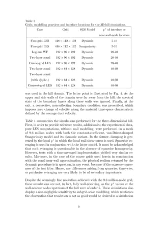
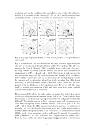
LES
Turbulent
boundary
layer eq.
wall shear stress
to LES
sublayer fed back
y+ interface
prescribed
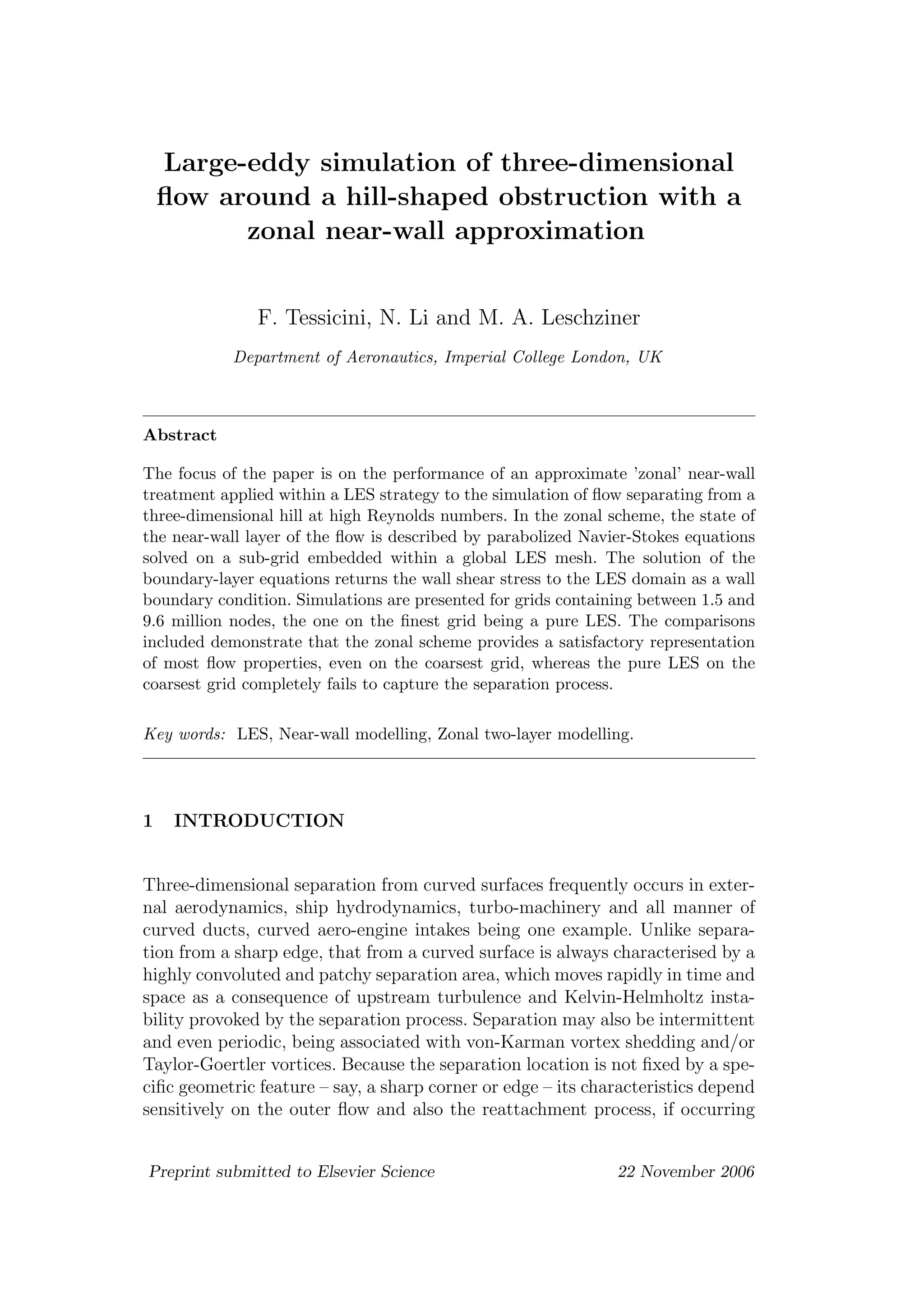
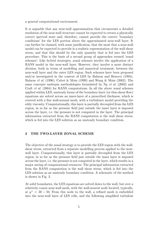
Fig. 2. Schematic of the two-layer zonal scheme.
boundary-layer equations are solved:
∂ρ ˜Ui
∂t
+
∂ρ ˜Ui
˜Uj
∂xj
+
∂ ˜P
∂xi
Fi
=
∂
∂y
[(µ + µt)
∂ ˜Ui
∂y
] i = 1, 3 (1)
where y denotes the direction normal to the wall and i identify the wall-parallel
directions (1 and 3). The left-hand-side terms are collectively referred to as
Fi.
In the present study, either none of the terms or only the pressure-gradient
term in Fi has been included in the near-wall approximation. The effects of
including the remaining terms are being investigated and will be reported
in future accounts. Depending on the terms included, equation (1) can be
solved algebraically or from differential equations, resulting in different degree
of simplifications. The wall shear stress is then evaluated from the solution.
The eddy viscosity µt is here obtained from a mixing-length model with near-
wall damping, as done by Wang & Moin (2002):
µt
µ
= κy+
w (1 − e−y+
w /A
)2
(2)
The boundary conditions for equation (1) are given by the unsteady outer-layer
solution at the first grid node outside the wall layer and the no-slip condition
at y = 0. Since the friction velocity is required in equation (2) to determine
y+
(which depends, in turn, on the wall-shear stress given by equation (1)),
an iterative procedure had to be implemented wherein µt is calculated from
equation (2), followed by an integration of equation (1).
6

7. 3 THE COMPUTATIONAL LES FRAMEWORK
The computational method rests on a general multiblock, collocated-storage
finite-volume scheme with non-orthogonal-mesh capabilities allowing the mesh
to be body-fitted. The scheme is second-order accurate in space, using cen-
tral differencing for advection and diffusion. Time-marching is based on a
fractional-step method, with the time derivative being discretized by a second-
order backward-biased approximation. The flux terms are advanced explicitly
using the Adams-Bashforth method. The provisional velocity field is then cor-
rected via the pressure gradient by a projection onto a divergence-free velocity
field. To this end, the pressure is computed as a solution to the pressure-
Poisson problem by means of a three-dimensional V-cycle multigrid algorithm
operating in conjunction with a successive line over-relaxation scheme. The
code is fully parallelised using MPI and was run on several multi-processor
computers with up to 256 processors. The procedure is more fully described
in Temmerman et al. (2002), and it has previously been used to investigate
the turbulence physics in a variety of generic flows, among them attached wall
jets (Dejoan et al., 2004) and the separated flow in a channel constricted by
streamwise periodic, two-dimensional hills (Froehlich et al., 2005).
4 THE SIMULATED CONFIGURATIONS
The three-dimensional circular hill, of height-to-base ratio of 4, is located
on the bottom wall of a duct, as shown earlier in Fig. 1. The size of the
computational domain is 16H×3.205H×11.67H, with H being the hill height.
The hill crest is 4H downstream of the inlet plane. One typical numerical mesh
is shown in Fig. 3.
L_x=16H
H
(c)
H
L_z = 11.67H
L_y=3.205H
(b)(a)
Fig. 3. Numerical grid: (a) perspective view of the computational domain (half);
(b) grid in y − z plane at x = 0; (c) grid in x − y plane at z = 0.
7

8. y/H
U/Uref
10-3
10-2
10-1
100
0
0.2
0.4
0.6
0.8
1
1.2
Simulation
Exp.
y/H
k/U2
ref
10-3
10-2
10-1
100
0
0.003
0.006
0.009
RANS
Exp.
Rescaled
Precursor
Fig. 4. The mean-velocity and turbulence-energy profiles at the inlet plane of the
three-dimensional hill domain.
The inlet conditions required particularly careful attention in this flow, be-
cause the inlet boundary layer is thick, roughly 50% of the hill height. As in-
dicated in Fig. 4, the mean flow was taken from a RANS simulation that accu-
rately matched the experimental conditions (Wang et al., 2004). The spectral
content was then generated separately by superposing onto the mean profile
fluctuations taken from a separate precursor boundary-layer simulation, per-
formed with a quasi-periodic recycling method, and rescaling the fluctuations
by reference to the ratio of the friction velocity values of the simulated bound-
ary layer, at Reθ = 1700, and the actual boundary layer ahead of the hill, at
Reθ = 7000. Although the fluctuations only roughly match the experimental
conditions at the inlet – as can be seen from the turbulence-kinetic-energy
profiles in Fig. 4 – specifying this reasonably realistic spectral representation
proved to be decisively superior to simply using uncorrelated fluctuations (Li
et al., 2005), even if the latter could be matched better to the experimental
profile of the turbulence energy. In particular, the simulation returned the cor-
rect mean-flow evolution of the boundary layer downstream of the inlet, and
the turbulence level was maintained at an approximately correct level, with a
slight downstream increase in level taking place, in contrast to the precipitous
decline observed when uncorrelated turbulence was prescribed. Also includes
the result of a second precursor simulation, performed at the correct Reynolds
number (Reθ = 7000), but over a grid that did not resolve the near-wall layer
and relied on a log-law wall model to approximate this layer. As seen, the
resulting turbulence-energy profile is not unambiguously superior to that aris-
ing from the rescaled lower-Reynolds-number simulation. It is arguable that a
better approach would have been to add a duct portion upstream of the inlet
and generate the inlet conditions, on the fly, by recycling the solution over
this duct portion, subject to the assumption of streamwise quasi-periodicity,
synchronously with the main LES solution over the hill domain. This approach
requires neither rescaling nor interpolation in space and time to account for
differences in mesh and time step between the precursor and the main simula-
tion. However, it would have been substantially more resource intensive, and
the outcome may well have been inferior in coarse-grid simulations in which
the near-wall layer would have had to be approximated by whatever scheme
8

9. Table 1
Grids, modelling practices and interface locations for the 3D-hill simulations.
Case Grid SGS Model y+ of interface or
near-wall-node location
Fine-grid LES 448 × 112 × 192 Dynamic 5-10
Fine-grid LES 448 × 112 × 192 Smagorinsky 5-10
Log-law WF 192 × 96 × 192 Dynamic 20-40
Two-layer zonal 192 × 96 × 192 Dynamic 20-40
Coarse-grid LES 192 × 96 × 192 Dynamic 20-40
Two-layer zonal 192 × 64 × 128 Dynamic 40-60
Two-layer zonal
(with dp/dxi) 192 × 64 × 128 Dynamic 40-60
Coarsest-grid LES 192 × 64 × 128 Dynamic 40-60
was used in the hill domain. The latter point is illustrated by Fig. 4. As the
upper and side walls of the domain were far away from the hill, the spectral
state of the boundary layers along these walls was ignored. Finally, at the
exit, a convective, non-reflecting boundary condition was prescribed, which
imposes zero change of velocity along the material time-space characteristic
defined by the average duct velocity.
Table 1 summarizes the simulations performed for the three-dimensional hill.
First, in order to provide reference results, additional to the experimental data,
pure LES computations, without wall modelling, were performed on a mesh
of 9.6 million nodes with both the constant-coefficient, van-Driest-damped
Smagorinsky model and its dynamic variant. In the former, damping is gov-
erned by the local y+
in which the local wall shear stress is used. Spanwise av-
eraging is used in conjunction with the latter model. It must be acknowledged
that such averaging is questionable in the absence of spanwise homogeneity.
However, tests with a time-averaged implementation yielded very similar re-
sults. Moreover, in the case of the coarse grids used herein in combination
with the zonal near-wall approximation, the physical realism returned by the
dynamic procedure is in question, in any event, because of the extreme coarse-
ness of the test filter. Hence, any differences arising from spanwise, time-wise,
or patchwise averaging are very likely to be of secondary importance.
Despite the seemingly fine resolution achieved with the 9.6 million-node grid,
these simulations are not, in fact, fully wall-resolving, as the y+
values at the
wall-nearest nodes upstream of the hill were of order 5. These simulations also
display a non-negligible sensitivity to subgrid-scale modelling, which reinforces
the observation that resolution is not as good would be desired in a simulation
9

10. that is beyond reproach. With wall models, the aspect ratio of the near-wall
grid is (supposedly) no longer a crucial constraint for LES, and major savings
in computational costs can be achieved by reducing the grid resolution in
the streamwise and spanwise directions. This was realised with meshes of
3.5 and 1.5 million nodes that were used with the zonal near-wall model.
Zonal-scheme simulations on the finer mesh were performed with and without
the pressure gradients included in the near-wall approximation. One further
pure LES computation was undertaken with the coarsest mesh of 1.5 million
nodes with no-slip conditions imposed at the walls. Finally, a simulation was
performed on the 3.5-million-node mesh with a conventional log-law-based
wall function at the hill wall. In the discussion to follow, the 9.6-million, 3.5-
million and 1.5-million node meshes are referred to as fine, coarse and coarsest,
respectively.
5 RESULTS AND DISCUSSION
Prior to a consideration of results obtained with the near-wall approximations,
attention is directed briefly to the pure LES solution on the 9.6-million-node
mesh, some of which have already been reported by Tessicini et al. (2005). As
noted earlier, by reference to Table 1, the near-wall resolution in this simula-
tion is insufficient, rendering it sensitive to sub-grid-scale modelling, especially
very close to the wall, where the asymptotic variation of the subgrid-scale
viscosity and stresses can be very important. This sensitivity is illustrated in
Fig. 5, which shows the mean velocity-vector fields across the hill centre-plane.
With the Smagorinsky model, separation occurs too early and gives rise to a
more extensive recirculation zone, which results in a slower pressure recovery
in the wake following the separation and consequent differences in the flow
fields downstream of reattachment. The dynamic model gives a shorter and
thinner recirculation zone, in better agreement with the experimental obser-
vations.
x/H
y/H
0 0.2 0.4 0.6 0.8 1 1.2 1.4 1.6 1.8 20
0.2
0.4
0.6
0.8
1
1.2
1
Fine-grid LES
(Smagorinsky)
x/H
y/H
0 0.2 0.4 0.6 0.8 1 1.2 1.4 1.6 1.8 20
0.2
0.4
0.6
0.8
1
1.2
1
Fine-grid LES
(Dynamic)
Fig. 5. Velocity fields across the centre-plane in the leeward of the hill - comparison
between fine-grid LES solutions using different SGS models and the experiment.
Despite the broadly satisfactory results derived with the dynamic model, some
caution is called for when assessing the physical fidelity of the results. As noted
earlier, the use of the dynamic model poses uncertainties when it is applied on
an under-resolving grid, because the near-wall variation of the Smagorinsky
10

11. constant, following spatial averaging, is quite sensitive to the near-wall grid,
and that grid is too coarse in the present LES computation. The fact that
the dynamic model nevertheless performs better than the constant-coefficient
variant is due to the former returning a better representation of the required
wall-asymptotic variation of the Smagorinsky viscosity (O(y3
)). An estimate
of the grid density required to yield a sufficiently well wall-resolved near-
hill representation suggests the need for a grid of 30 − 50 million nodes, an
extremely expensive proposition in view of the modest Reynolds number.
Statistical results obtained with the wall-functions and zonal two-layer near-
wall approximation are given in Figs. 6 to 15. In all these figures, the version
of the zonal scheme used is that without the pressure gradient; separate com-
parisons between the versions that include and exclude the pressure gradient
will be given at the end. These figures show, respectively, profiles of the pres-
sure coefficient along the hill surface at the centre-plane, pressure contours
on the hill surface, velocity-vector fields across the centre-plane, flow-topology
maps on the leeward side of the hill, velocity profiles in the cross-flow plane
at the downstream location x/H = 3.63 and contours and profiles of turbu-
lent kinetic energy at that same location at which experimental data are also
available. Furthermore, some images of instantaneous flow features are given
in Figs. 16 to 17, and these will support a discussion of some specific features
of the unsteady motions.
x/H
Cp
1 2 3
-0.6
-0.4
-0.2
0
0.2
0.4
Experiment
Fine-grid (Smagorinsky)
Fine-grid (Dynamic)
Coarse-grid, Log Law
Coarse-grid, Two-layer
(b)
x/H
Cp
1 2 3
-0.6
-0.4
-0.2
0
0.2
0.4
Experiment
Coarse-grid, pure LES
Coarsest-grid, Two-layer
Coarsest-grid, pure LES
(c)
x/H
Cp
-2 0 2 4 6 8 10
-1
-0.5
0
0.5 (a)
Fig. 6. Pressure coefficient along the hill surface at the centre-plane: (a) full view;
(b) and (c) zoomed-in view around the region where separation occurs.
Fig. 6(a) shows that, except for the coarsest-grid (1.5 million nodes) pure
LES, all simulations predict the pressure-coefficient distribution reasonably
well. The magnified views provided in Fig. 6(b) and (c) reveal, in particular,
that the inflexion in the Cp curves, associated with the weak separation on
the leeward side of the hill, is well captured. The benefit of using wall models
becomes especially evident in the case of extremely poor spatial resolution,
on the 1.5 million-node mesh, where the use of no-slip conditions results in
a grossly erroneous prediction of the separation process. In fact, as will be
shown below, a fully attached flow is predicted, and an excessively fast pressure
recovery after the hill crest is returned. In contrast, applying a wall model on
11

12. the coarsest grid results in the resolution of the separation process and thus
a reasonable representation of the pressure-recovery process.
X
Z
-4 -3 -2 -1 0 1 2 3
-2
-1
0
1
2
1
1
2
22
33
3
4
4
4
4
55
5
5
66
6
6
77
77
7
8
88
8
8
99
99
9
10
10
1010
10
11
11
11
111111
12
12
12
1212
12
12
13
13
13
13
13
13
13
13
14
14
14
15
15
x/H
z/H
-4 -3 -2 -1 0 1 2 3
-2
-1
0
1
2
Level P
15 3.08E-01
14 2.13E-01
13 1.19E-01
12 2.40E-02
11 -7.05E-02
10 -1.65E-01
9 -2.60E-01
8 -3.54E-01
7 -4.49E-01
6 -5.43E-01
5 -6.36E-01
4 -7.32E-01
3 -8.27E-01
2 -9.21E-01
1 -1.02E+00
Coarse-grid
Two-layer
1
1
2
2
2
3
3
3
4
4
4
5
5
55
66
66
77
77
7
88
8
88
9
9
9
9
9
10
10
10
1010
10
11
11
11
111111
12
12
12
121213
13
13
13
13
13
13
13
13
14
14
14
14
14
15
15
15
x/H
z/H
-4 -3 -2 -1 0 1 2 3
-2
-1
0
1
2
Level P
15 3.08E-01
14 2.13E-01
13 1.19E-01
12 2.40E-02
11 -7.05E-02
10 -1.65E-01
9 -2.60E-01
8 -3.54E-01
7 -4.49E-01
6 -5.43E-01
5 -6.36E-01
4 -7.32E-01
3 -8.27E-01
2 -9.21E-01
1 -1.02E+00
Fine-grid LES
(Dynamic)
X
Z
-4 -3 -2 -1 0 1 2 3
-2
-1
0
1
2
1
1
2
2
2
3
3
3
44
4
5
5
5
6
6
6
6
77
7
77
8
88
88
99
9
9
9
10
10
10
10
10
10
11
11
11
11
1111
12
12
12
12
1212
12
12
13
13
13
13
13
13
13
13
14
14
14
14
15
15
x/H
z/H
-4 -3 -2 -1 0 1 2 3
-2
-1
0
1
2
Level P
15 3.08E-01
14 2.13E-01
13 1.19E-01
12 2.40E-02
11 -7.05E-02
10 -1.65E-01
9 -2.60E-01
8 -3.54E-01
7 -4.49E-01
6 -5.43E-01
5 -6.36E-01
4 -7.32E-01
3 -8.27E-01
2 -9.21E-01
1 -1.02E+00
Coarse-grid
Log Law
Fig. 7. Contours of the pressure coefficient on the hill. Comparison between the
experiment, two coarse-grid simulations and one fine-grid simulation.
Broader views of the pressure field are given in Fig. 7, which show contour
plots of cp above the hill. The circles in these plots indicate the foot of the hill.
The predicted fields, two derived from coarse-grid simulations and one from
a fine-grid simulation, agree well with the experimental results of Simpson et
al. (2002).
According to the experiment, the flow in the symmetric plane separates about
1 hill height (x/H = 0.96) after passing over the hill crest. The separation zone
is very shallow, and the flow reattaches at the foot of the hill at x/H = 2.0.
In the fine-grid simulations as well as all simulations using wall models, the
size and extent of the recirculation zone on the leeward side of the hill agree
fairly well with the experimental results, as shown in Fig. 8. With poor spatial
x/H
y/H
0 0.2 0.4 0.6 0.8 1 1.2 1.4 1.6 1.8 20
0.2
0.4
0.6
0.8
1
1.2
1
Fine-grid LES
(Dynamic)
x/H
y/H
0 0.2 0.4 0.6 0.8 1 1.2 1.4 1.6 1.8 20
0.2
0.4
0.6
0.8
1
1.2
1
Coarse-grid
Log Law
x/H
y/H
0 0.2 0.4 0.6 0.8 1 1.2 1.4 1.6 1.8 20
0.2
0.4
0.6
0.8
1
1.2
1
Coarse-grid
Two-layer
x/H
y/H
0 0.2 0.4 0.6 0.8 1 1.2 1.4 1.6 1.8 20
0.2
0.4
0.6
0.8
1
1.2
1
Coarse-grid
pure LES
x/H
y/H
0 0.2 0.4 0.6 0.8 1 1.2 1.4 1.6 1.8 20
0.2
0.4
0.6
0.8
1
1.2
1
Coarsest-grid
pure LES
Fig. 8. Velocity field across the centre-plane in the leeward of the hill - compar-
ison between pure LES solutions, wall-model solutions and the experiment. The
zero-U-velocity lines are good indications of the recirculation zone size.
12

13. resolution and no-slip conditions, the recirculation zone predicted is either too
small - as is the case for the coarse-grid LES on the 3.5 million-node mesh -
or entirely absent - as is the case for the 1.5-million-node coarsest mesh.
x/H
z/H
0 0.5 1 1.5 2
-2
-1.5
-1
-0.5
0
Fine-grid LES
(Dynamic)
X
Z
0 0.5 1 1.5 2
-2
-1.5
-1
-0.5
0
x/H
z/H
0 0.5 1 1.5 2
-2
-1.5
-1
-0.5
0
Coarse-grid
Log Law
X
Z
0 0.5 1 1.5 2
-2
-1.5
-1
-0.5
0
x/H
z/H
0 0.5 1 1.5 2
-2
-1.5
-1
-0.5
0
Coarse-grid
Two-layer
X
Z
0 0.5 1 1.5 2
-2
-1.5
-1
-0.5
0
x/H
z/H
0 0.5 1 1.5 2
-2
-1.5
-1
-0.5
0
Coarsest-grid
Two-layer
Fig. 9. Topology maps predicted by the wall models, relative to the pure LES and
experiment.
Fig. 9 demonstrates that the simulations with the near-wall approximations
also give a broadly faithful representation of the flow topology. The LDV ex-
periment by Byun & Simpson (2005) reveal the presence of a pair of counter-
rotating vortices detaching from the leeward side of the hill and centred at
approximately x/H = 1.2 and z/H = ±0.7. This feature is well captured by
the simulations, especially by those involving wall models. With the combi-
nation of the coarsest-grid and the no-slip conditions, the topology is seen to
be characterized by streaklines identifying a fully attached flow. This is not
surprising, as the wall-normal height of the cells closest to the wall are com-
parable with the thickness of the separation zone. However, with the zonal
model, a realistic representation of the wall shear stress is returned, and the
correct vortical structure is recovered.
Downstream of the hill, in the wake region, one major flow feature is a pair of
counter-rotating streamwise vortices, shown in Fig. 10. These originate from
the vorticity in the boundary layer upstream of the hill and generated from the
hill itself. The simulations are in fairly close agreement with the experimental
data. One discrepancy arises, however, around the location y/H = 0.7 and
z/H = ±0.4, where the LDV measurement clearly indicates the existence of
secondary vortices. Neither the simulations performed by the present authors,
nor the CFD studies performed by other researchers, i.e. Benhamadouche et al.
(2005), predict these secondary vortices. A Proper Orthogonal Decomposition
(POD) (Berkooz et al, 1993), discussed later, suggests that the vorticity shed
from the focus on the hill surface is propagated approximately to the location
13

14. z/H
y/H
-2.5 -2 -1.5 -1 -0.5 00
0.5
1
Coarse-grid
Log Law
z/H
y/H
-2.5 -2 -1.5 -1 -0.5 00
0.5
1
Coarse-grid
Two-layer
z/H
y/H
-2.5 -2 -1.5 -1 -0.5 00
0.2
0.4
0.6
0.8
1
Fine-gird LES
(Dynamic)
Fig. 10. Velocity vectors at x/H = 3.63 in the wake.
at which the measurements return the secondary vortex. However, in the sim-
ulation, this vortex is not visible in the time-averaged transverse-velocity field.
Hence, if the measurements are correct (and there are some significant doubts
about this region, for reasons explained below), it must be concluded that lack
of resolution prevents the secondary vortex from being visibly captured; the
vorticity may be present, but may be smeared to an extend preventing the
vortical feature from becoming evident.
0 0.4 0.8
U/Uref
0
0.2
0.4
0.6
0.8
1
y/H
0 0.4 0.8
U/Uref
|z/H|=0.33z/H=0.00 |z/H|=0.65
Exp. (LDV)
Exp. (LDV)
Log Law
Two-layer Zonal
LES (Dynamic)
LES (Smag.)
Exp. (HWA)
Coarse-grid LES
0 0.4 0.8
U/Uref
-0.1 0 0.1
W/Uref
0
0.2
0.4
0.6
0.8
1
y/H
|z/H|=0.33 |z/H|=0.65
-0.1 0 0.1
W/Uref
Exp. (LDV)
Log Law
Two-layer Zonal
LES (Dynamic)
LES (Smag.)
Fig. 11. Mean streamwise- and spanwise-velocity profiles at various spanwise loca-
tions on the downstream plane x/H = 3.63.
To examine the wake statistics in detail, streamwise- and spanwise-velocity
profiles at various spanwise locations on the plane x/H = 3.63 are shown in
Fig. 11. Three sets of experimental data are included: two obtained with LDV,
on either side of the centre-plane, and the third obtained by means of HWA in
the same facility by Ma & Simpson (2005). A magnified view of the streamwise
velocity on the centre plane, providing a greater degree of differentiation, is
given in Fig. 12. Consistent with the earlier results, the excessively large sepa-
ration zone, returned by the fine-grid LES with the Smagorinsky model, goes
hand-in-hand with a too slow recovery of the flow in the wake, so that the
14

15. 0 0.2 0.4 0.6 0.8 1
U/Uref
0
0.2
0.4
0.6
0.8
1
y/H
Exp. (LDV)
Coarse-grid, Log Law
Coarse-grid, Two-layer Zonal
Fine-grid LES (Dynamic)
Fine-grid LES (Smag.)
Exp. (HWA)
Coarse-grid, pure LES
Coarsest-grid, Two-layer Zonal
Fig. 12. Magnified view of the mean streamwise velocity distribution at z/H = 0
on the downstream plane x/H = 3.63.
near-wall streamwise velocity is under-predicted in that simulation. On the
other hand, when a simulation fails to capture the separation (as is the case
with the coarse-grid and no-slip conditions), or when the reattachment occurs
too early at the foot of the hill, the flow recovers at an excessive rate and the
streamwise velocity is over-predicted. All the computations performed either
with the two-layer zonal model or with the log-law WF generally give much
better results than those performed with the no-slip condition. In the region
far away from the wall, beyond y/H = 0.4, the predicted velocity profiles are
noticeably different from the experimental LDV data, while they agree closely
with the HWA measurements. The differences between the two sets of exper-
imental data are obviously disconcerting. The present authors are only able
to report that the experimental investigators have expressed their view, in a
private communication, that the LDV data are erroneous in regions remote
from the wall, due to seeding problems, and that the HWA data are to be
preferred.
Fig. 13 shows the z-wise distribution of the friction velocity uτ (= τwall/ρ0.5
),
normalized by the velocity at x/H = 2 and the duct centre, Uref , on the lower
0 0.5 1 1.5 2 2.5 3
z/H
0.01
0.02
0.03
0.04
0.05
Uτ/Uref
Fine−grid LES (dynamic)
Coarse−grid , Two−layer Zonal
Coarsest−grid, Two−layer Zonal
Exp., z<0
Exp., z>0
Fig. 13. Variation of uτ /Uref across the flow at x/H = 3.63.
15

16. wall at x/H = 3.63 in the wake, obtained by time-averaging the instantaneous
wall shear stress that is returned by the wall model through the inner-layer
velocity profiles. Comparisons are made among the fine-grid result, two zonal-
model results and the experiment. The wall shear stress is the principal output
sought from the wall model, and it is therefore of particular interest in the
context of this study. It is also an especially sensitive indicator of the near-wall
conditions and a variable that displays more prominently than other mean-flow
quantities a slow statistical convergence. This is the rather ’noise’ appearance
of the distributions in Fig. 13, also linked to the undulations in the near-wall
streamwise velocity seen in Fig. 12. While even longer integration times than
those given at the end of Section 4 would have led to smoother variations,
especially for the 3.5- and 9.5-million-node simulations, the attendant costs
for the finer were deemed to be excessive relative to anticipated benefits.
As seen, there is a fair agreement among the skin-frictions distributions aris-
ing from the simulations and also with the experimental data. Curiously, the
largest differences arise beyond the base of the hill, z/H > 2, i.e. outside
the most complex flow region recovering from separation. With a spanwise
grid-expansion ratio being only 1.027, the cell aspect ratio at z/H = 2 is not
much higher than in the central region, reaching only 12.6 at z/H=4. Hence,
the resolution in the outer area is not seriously inferior to that in the central
duct portion. On the assumption that the experimental data are correct, it
is possible that the discrepancies reflect a failure of the simulation to resolve
the effects of (relatively weak) legs of the horseshoe vortex on either side of
the hill, associated with the vorticity in the upstream boundary layer. The
experiments (see Fig. 14, discussed later) show a bulge-like region of elevated
turbulence energy close to the wall around z/H = 2, while the simulation only
hints at this feature. As near-wall turbulence tends to go hand-in-hand with
the wall shear stress in boundary layers, the experimental trends in this region
seem credible. Another possible source for the differences is that the near-wall
turbulence state is perhaps more sensitive than in others to the ability of
the simulation to resolve the slowly evolving boundary-layer structure and its
readjustment from the approximate state prescribed at the inlet. Close to the
centre-plane, the fine-grid simulation goes some way towards capturing the
distinct peak of the wall shear-stress, presumably reflecting the high turbu-
lence activity originating from the reattachment area upstream and convected
downstream. This feature is not resolved by the zonal-model simulations, be-
cause turbulence transport is not accounted for in the near-wall, and there is
no mechanism for sensitising the shear stress to the turbulence level above the
near-wall layer.
Fig. 14 shows contours of turbulent kinetic energy, normalised by the square
of the free-stream velocity, on the same cross-wake plane considered above.
Included in the figures are numerical results obtained from the 3.5-million-node
simulations performed with the log-law WF and the two-layer zonal scheme,
16

17. z/H
y/H
-2.5 -2 -1.5 -1 -0.5 0 0.5 1 1.5 2 2.50
0.4
0.8
1.2
z/H
y/H
-2.5 -2 -1.5 -1 -0.5 0 0.5 1 1.5 2 2.50
0.4
0.8
1.2
0.038
0.034
0.03
0.026
0.022
0.018
0.014
0.01
0.006
0.002
Coarse-grid
Log Law
Coarse-grid
Two-layer
Fig. 14. Turbulent kinetic energy distribution at x/H = 3.63. Top: LDV measure-
ment; middle: HWA measurement; bottom: simulations.
and these are compared to two sets of experimental results, one obtained
by LDV (top plot) and the other with HWA (middle plot) 1
. Here again,
disconcertingly large differences between the two sets of experimental data
are evident, and it is recalled that the experimental investigators attribute
this to seeding-related errors in the LDV measurements. The LDV data show
the maximum of turbulence energy to occur around y/H = 0.7 − 0.8 (see
also Fig. 15), while the maximum returned by the HWA measurements is at
around y/H = 0.3. More generally, the LDV data imply that the region of
high turbulence activity is substantially further from the lower wall, relative
to that suggest by the HWA results.
The computations return a broadly satisfactory agreement with the HWA
data, but not the LDV field. With the zonal model, the lateral extent the
1 The arrows superimposed on the contours do not identify transverse motion,
but represent diffusive transport fluxes of turbulence energy, associated with triple
correlations
17

18. 0 0.02 0.04 0.06
k/Uref
2
0
0.2
0.4
0.6
0.8
1
1.2
y/H
0 0.02 0.04 0.06
k/Uref
2
Exp. (LDV)
Exp. (LDV)
LES (Dynamic)
Two−layer Zonal
0 0.02 0.04 0.06
k/Uref
2
z/H=0.00 |z/H|=0.33 |z/H|=0.65
Fig. 15. Turbulent kinetic energy profiles at various spanwise locations on the down-
stream plane x/H = 3.63.
turbulent wake is better predicted, but the central portion of the wake is
more highly turbulent than the measured level - roughly 0.035 as compared
to 0.025). Fig. 15 provides a comparison of computed and measured profiles
of turbulence energy at three spanwise locations, all within the streamwise
plane x/H = 3.63 - that is, the same plane to which Fig. 10 relates. The
measured profiles suggest two principal regions of high turbulence activity:
one close to the wall, around y/H = 0.2, and the other much higher, at
around y/H = 0.8, the latter being consistent with the top contour plot
in Fig. 10 which arises from the LDV measurements. The maximum at the
higher elevation is rather surprising on several grounds. First, the velocity
profiles, Fig. 11, show that the shear strain at this elevation is rather weak -
certainly too weak to explain why local shear-induced generation would cause
the turbulence level to be above that in the wake of the separated region
in which turbulence is strongly elevated by convection of turbulence from
upstream. Second, the field of transverse motion, Fig. 10, suggests the presence
of rather weak convective transport of turbulence from the lower-wall layer
towards the upper part - and in any event, the simulation reproduces (if not
over-estimates) this motion that would be the cause for this transport. Third,
Fig. 8 suggests that the motion in the centre-plane, in the leeward side, is
predominantly downwards, and this process is also indicated by the diverging
streaklines around the centreline behind the hill, not included herein. This
downward motion would thus tend to transport turbulence from upper regions
towards the wall, rather than supply the upper region with highly turbulent
fluid. A feature that might be linked to the elevated turbulence energy at
around y/H = 0.7 is the secondary vortex found at the location z/H = 0.4,
y/H = 0.7 by the LDV measurement in the transverse velocity field shown in
Fig. 10. It has been conjectured in an earlier part of this discussion - partly
on the basis of a POD of the velocity field, discussed later - that this vortex
18

19. reflects the ejection of vortical fluid from the recirculation region away from the
leeward side of the hill. This ejection, which must be assumed to be present, is
evidently not resolved by the simulations, or is too diffuse to be brought out.
Whether and how the two features are linked is not possible to be determined
from the data so far available. Indeed, it is unclear why the HWA experiments
fail to resolve both these features.
While the statistical results of the flow are evidently in fairly good agreement
with the experiments, a closer examination of the turbulent structures is de-
sirable to shed light on some of the detailed physics and dynamics of the flow.
One particularly influential unsteady process is the shedding (or ejection) of
large-scale vortical structures from the leeward side of the hill and their in-
teractions with the downstream boundary layer. This has been the subject of
discussion in previous experimental studies. For example, Byun and Simpson
(2005) have observed very-low-frequency, large-amplitude spanwise ’meander-
ing’ motion of the shed vortex structures. Efforts to visualize, identify and
analyze these coherent structures from the simulations are far from straight-
forward, due to the complexity of the flow. Conventional methods for detecting
coherent vortices, such as the Q− and λ2 criteria, do not work effectively for
this flow. Also, the subtle nature and the low frequency of any periodic process
make its detection a difficult task. In the present paper, we confine ourselves
to giving a few observations on some unsteady motions in the flow. A detailed
study of this subject will be reported elsewhere.
Fig. 16. Temporal evolution of pressure field above the hill on the center plane.
Fig. 16 shows time-space plots of the hill-surface pressure along the line
z/H = 0. The figure suggests the existence of a weak form of shedding. Thus,
an almost periodic variation of the pressure field is observed, with a non-
dimensional frequency fH/Uref ≈ 0.83. Fig. 17 shows the temporal evolution
of the near-wall streamwise velocity at z/H = ±0.4 at either side of the hill.
This reveals a temporal pattern consistent with that shown in Fig. 16, and it
19

20. Fig. 17. Temporal evolution of vortical structures on top of the hill indicating that
the flow is symmetric at instantaneous level.
also indicates that the shedding is nearly symmetrical, rather than alternating.
Clearly, this type of periodicity is unrelated to conventional vortex shedding
behind bluff bodies, and their origin is a subject of ongoing studies. Although
the vortical structures shed from the hill are obscured by a broad range of
smaller-scale motions and do not reveal themselves in conventional visualisa-
tion or in the statistical results, they can be detected and visualized through
the reconstruction of most the energetic modes of motion obtained by POD.
At the time of writing, these studies are still incomplete, but Fig. 18 gives a
flavour of the outcome of a POD analysis based on 700 samples covering a
period of 160 time units (Uref /H). The analysis includes the lowest four POD
modes (in addition to mode 0, representing the mean flow) extracted from
the data of the simulation on the 3.5-million-node mesh. The figure shows the
cores of vortical structures, forming a family of Ω-shaped vorticity lines, that
originate from the focal points on the hill (included in the upper-left inset),
are ejected into the wake and evolve in space in a manner similar to hair-
pin vortices. The upper-right inset shows a pair of counter-rotating structures
through streaklines constructed with the low-order POD representation of the
transverse velocity in the downstream plane x/H = 2.2. These results support
the earlier statement that the nearly periodic shedding process is symmetric.
All the results presented so far for the zonal two-layer model were obtained
with the pressure gradient omitted from the solution of the wall-layer equations
(1). Clearly, a more general formulation would include the pressure gradient
and also the convective terms. The latter extension is the subject of ongoing
work. Here, the consequences of including the pressure gradient are briefly
20

21. Fig. 18. Flow field reconstructed using the five most energetic POD modes based on
the coarse-grid LES. Upper left: streaklines at ∆y = 0.01. Upper right: streaklines
at x/H = 2.2
considered. Thus, Fig. 19 compares the topology on the leeward portion of the
hill surface predicted without and with the pressure gradient in the near-wall
model. The two simulations are seen to produce similar global features with
slightly different structures in the vicinity of the foci and the reattachment
point. Significantly, the inclusion of the pressure gradient leads to a slight shift
of the separation line towards the hill crest. This is the expected qualitative
response, for the adverse pressure gradient in the separation region results
x/H
z/H
-1 -0.5 0 0.5 1 1.5 2 2.5 3 3.5
-2
-1.5
-1
-0.5
0
0.5
1
1.5
2
x/H
z/H
-1 -0.5 0 0.5 1 1.5 2 2.5 3 3.5
-2
-1.5
-1
-0.5
0
0.5
1
1.5
2
Fig. 19. The flow topology predicted by two-layer zonal model without (left) and
with (right) the pressure gradient term.
21

22. in a reduction in the predicted wall shear stress returned by the extended
formulation. Other than these differences, respective flow statistics derived
from the two simulations, especially those downstream of the hill in the wake
area, have been found to be close, and these comparisons are not included
herein. It is appropriate to finally point out that the effects of modifying the
wall model, detrimental or beneficial, cannot easily be identified or isolated
without the ambiguity that arises from other numerical issues. In particular,
all simulations are under-resolved, and the role of the subgrid-scale model
in the under-resolved environment has already been pointed out. This is not
only a problem with the present extension, but also with that involving the
inclusion of the convection terms in equation (1). The latter makes the model
non-linear, non-local and thus much more expensive to solve.
6 CONCLUSIONS
The emphasis of this study has been on the ability of LES to reproduce the
challenging process of three-dimensional separation from a gently curved sur-
face. This is, arguably, a very important generic configuration in the context
of off-design external aerodynamics. Received wisdom is that such any flow
of the type examined is highly sensitive to the details in the description up-
stream of the separated region - i.e. the structure of the boundary layer - and
the accuracy with which the near-wall layer is resolved.
In the present study, simulations have been performed with grids which, with-
out doubt, do not fully resolve the flow, in so far as a not insignificant pro-
portion of the turbulence activity is not resolved, but is filtered and/or repre-
sented by the subgrid-scale model, even with the finest grid of close to 10 mil-
lion nodes. Moreover, the near-wall region was modelled with a rather crude
approximation, which may be regarded as a variation of log-law-based wall
functions. Yet, the results obtained are pleasingly close to the experimental
observations – certainly much closer than achieved with RANS models.
As the predictive quality depends significantly on the resolution of the LES
grid, the performance of the subgrid-scale model, especially in the ill-resolved
near-wall region, and the spectral description of the inflow, it is difficult to
unambiguously isolate and quantify the role of the near-wall model in the
favourable outcome of the simulations. However, it is reasonably clear that
prescribing, simplistically, a no-slip condition at the wall in coarse-grid sim-
ulations and extracting the shear stress from the predicted near-wall velocity
gradient is decidedly inferior to using even simple near-wall models that return
reasonable values for the wall shear stress. This is reflected by the outcome
of simulation with the coarsest grid of 1.5 million nodes, in which case the
use of a no-slip condition resulted in separation being entirely missed. With
22

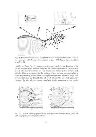
23. the near-wall models examined herein, most flow properties are fairly well -
indeed, surprisingly well - predicted. In particular, the extent of the separated
zone on the leeward side of the hill, the surface-pressure field and the flow
topology are well reproduced, and the wake structure is also broadly correct.
Inclusion of the pressure gradient in the near-wall model has not been found
to have a decisive effect on predictive accuracy.
A specific experimentally-observed feature that has not been resolved is a pair
of small secondary vortices lying next to the much larger and dominant pri-
mary vortices associated with the interaction of the upstream boundary layer
with the hill. These vortices could be the ’foot prints’ of the vertical separation
originating from the focal points on the leeward side of the hill. A POD study
lends support to this supposition, but the strength of the secondary vortices
is evidently too low or the vorticity too diffused to be visible in the time-mean
transverse-velocity field. On the other hand, there are justifiable doubts about
the validity of the LDV data in the region containing the measured secondary
vortices.
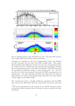
A limited examination of unsteady fields revealed an intriguing periodicity in
the pressure and velocity fields downstream of the hill crest. This does not seem
to be related in any obvious way to conventional shedding: the frequency of
the periodic features does not agree with that of shedding behind bluff bodies,
and there is no alternate motion suggestive of conventional vortex shedding.
The results of the POD also indicate that the shedding is symmetric.
7 ACKNOWLEDGEMENTS
This work was undertaken, in part, within the DESider project (Detached
Eddy Simulation for Industrial Aerodynamics). The project is funded by
the European Union and administrated by the CEC, Research Directorate-
General, Growth Programme, under Contract No. AST3-CT-2003-502842.
N. Li and M.A. Leschziner gratefully acknowledge the financial support pro-
vided by BAE Systems and EPSRC through the DARP project ”Highly Swept
Leading Edge Separation”.
References
[1] Balaras, E., Benocci, C., 1994. Subgrid-scale models in finite difference
simulations of complex wall bounded flows. Applications of Direct and Large
Eddy Simulation, AGARD, 2-1-2-6.
23

24. [2] Balaras, E., Benocci, C., Piomelli, U., 1996. Two-layer approximate boundary
conditions for large-eddy simulations. AIAA Journal, 34 (6), 1111-1119.
[3] Benhamadouche S., Uribe J., Jarrin N., Laurence D., 2005. 4th
International Symposium on Turbulence and Shear Flow Phenomena (TSFP4),
Williamsburg, 325-330.
[4] Berkooz, G., Holmes, P., Lumley, J.L., 1993. The Proper Orthogonal
Decomposition in the Analysis of Turbulent Flows. Annual Review of Fluid
Mechanics, 25 (1), 539-575.
[5] Byun, G., Simpson, R.L., 2005. Structure of three-dimensional separated flow
on an axisymmetric bump. AIAA Paper, 2005-0113.
[6] Cabot, W., Moin, P., 1999. Approximate wall boundary conditions in the
large eddy simulation of high Reynolds number flow. Flow, Turbulence and
Combustion, 63, 269-291.
[7] Chaouat B., Schiestel R., 2005. A new subgrid-scale stress transport model and
its application to LES of evolving complex turbulent flows. 4th Int. Symp. on
Turbulence and Shear Flow Phenomena (TSFP4), Williamsburg, 1061-1066.
[8] Craft, T.J., Gant, S.E., Iacovides, H., Launder, B.E., 2004. A new wall
function strategy for complex turbulent flows. Numerical Heat Transfer, Part
B: Fundamentals, 45 (4), 301-318.
[9] Davidson, L., Billson, M., 2006. Hybrid LES-RANS using synthesized turbulent
fluctuations for forcing in the interface region. To appear in International
Journal of Heat and Fluid Flow.
[10] Davidson, L., Dahlstrom, S., 2004. Hybrid LES-RANS: an approach to make
LES applicable at high Reynolds number. In Procs CHT-04 Advances in
Computational Heat Transfer III, G. de Vahl Davis and E. Leonardi (eds.),
Norway.
[11] Deardorff, J.W., 1970. A numerical study of three-dimensional turbulent
channel flow at large Reynolds numbers. Journal of Fluid Mechanics, 41, 453-
480.
[12] Dejoan, A., Leschziner, M.A., 2005. Large eddy simulation of a plane turbulent
wall jet. Physics of Fluids, 17 (2), paper 025102.
[13] Froehlich, J., Mellen, C., Rodi, W., Temmerman, L., Leschziner, M.A., 2005.
Highly resolved large eddy simulation of separated flow in a channel with
streamwise periodic constrictions. Journal of Fluid Mechanics, 526, 19-66.
[14] Helman, J.L., Hesselink, L., 1990. Surface representations of two- and
three-dimensional fluid flow topology, Proceedings of the 1st conference on
Visualization ’90, IEEE Computer Society Press, 6-13.
[15] Hoffmann, G., Benocci, C., 1995. Approximate wall boundary conditions for
large-eddy simulations. Advance in Turbulence V, Benzi, R. (Ed.), 222-228.
24

25. [16] Li, N., Wang, C., Avdis, A., Leschziner, M.A., Temmerman, L., 2005. Large
eddy simulation of separation from a three-dimensional hill versus second-
moment-closure RANS modelling. 4th Int. Symp. on Turbulence and Shear
Flow Phenomena (TSFP4), Williamsburg, 331-336.
[17] Ma, R., Simpson, R.L., 2005. Characterization of turbulent flow downstream
of a three-dimensional axisymmetric bump. 4th Int. Symp. on Turbulence and
Shear Flow Phenomena (TSFP4), Williamsburg, 1171-1176.
[18] Ng, E.Y.K., Tan, H.Y., Lim, H.N., Choi, D., 2002. Near-wall function for
turbulence closure models. Computational Mechanics, 29, 178-181.
[19] Patel, N., Stone, C., Menon, S., 2003. Large-eddy simulation of turbulent flow
over an axisymmetric hill, AIAA Paper, 2003-0967.
[20] Perry, A.E., Chong, M.S., 1987. A description of eddying motions and flow
patterns using critical-point concepts, Ann. Rev. Fluid Mech., 19, 125-155.
[21] Persson, T., Liefvendahl M., Bensow, R.E., Fureby C., 2006. Numerical
investigation of the flow over an axisymmetric hill using LES, DES and RANS.
Journal of Turbulence, 7 (4), 1-17.
[22] Piomelli, U., Balaras, E., Pasinato, H., Squires, K.D., Spalart, P.R., 2003. The
inner-outer layer interface in large-eddy simulations with wall-layer models.
International Journal of Heat and Fluid Flow, 24 (4), 538-550.
[23] Schiestel, R., Dejoan, A., 2005. Towards a new partially integrated transport
model for coarse grid and unsteady turbulent flow simulations. Theoretical and
Computational Fluid Dynamics, 18 (6), 443-468.
[24] Schumann, U., 1975. Subgrid scale model for finite difference simulations of
turbulent flows in plane channels and annuli. Journal of Comp. Phys., 18, 376-
404.
[25] Simpson, R.L., Long, C.H., Byun, G., 2002, Study of vortical separation from
an axisymmetric hill. International Journal of Heat and Fluid Flow, 140 (2),
233-258.
[26] Spalart, P.R., Jou, W.-H., Strelets, M., Allmaras, S.R., 1997. Comments on the
feasibility of LES for wings and on the hybrid RANS/LES approach. Advances
in DNS/LES, 1st AFOSR International Conference on DNS/LES, Greyden
Press, 137-148.
[27] Temmerman, L., Hadziabli´c, M., Leschziner, M.A., Hanjali´c, K., 2005. A
hybrid two-layer URANS-LES approach for large eddy simulation at high Re.
International Journal of Heat and Fluid Flow. 26 (2), 173-190.
[28] Temmerman, L., Leschziner, M.A., Hanjali´c, K., 2002. A-priori studies of
a near-wall RANS model within a hybrid LES/RANS scheme. Engineering
Turbulence Modelling and Experiments. Rodi, W. and Fueyo, N. (Eds.),
Elsevier, 317-326.
25

26. [29] Temmerman, L., Leschziner, M.A., Mellen, C.P., Frohlich, J., 2003.
Investigation of wall-function approximations and subgrid-scale models in
large eddy simulation of separated flow in a channel with streamwise periodic
constrictions. International Journal of Heat and Fluid Flow. 24 (2), 157-180.
[30] Temmerman, L., Wang, C., Leschziner, M.A., 2004. A comparative study of
separation from a three-dimensional hill using LES and second-moment-closure
RANS modeling. European Congress on Computational Methods in Applied
Sciences and Engineering, ECCOMAS.
[31] Tessicini, F., Li, N., Leschziner, M.A., 2005. Zonal LES/RANS modelling of
separated flow around a three-dimensional hill. ERCOFTAC Workshop Direct
and Large-Eddy Simulation-6, Poitiers.
[32] Tessicini, F., Temmerman, L., Leschziner, M.A., 2006. Approximate near-wall
treatments based on zonal and hybrid RANS-LES methods for LES at high
Reynolds numbers. International Journal of Heat and Fluid Flow, 27 (5), 789-
799.
[33] Wang, C., Jang, Y.J., Leschziner, M.A., 2004. Modelling 2 and 3-dimensional
separation from curved surfaces with anisotropic-resolving turbulence closures.
International Journal of Heat and Fluid Flow. 25, 499-512.
[34] Wang, M., Moin, P., 2002. Dynamic wall modelling for large-eddy simulation
of complex turbulent flows. Physics of Fluids. 14 (7), 2043-2051.
[35] Werner, H., Wengle, H., 1991. Large-eddy simulation of turbulent flow over and
around a cube in a plate channel. 8th Symposium on Turbulent Shear Flows,
155-168.
26