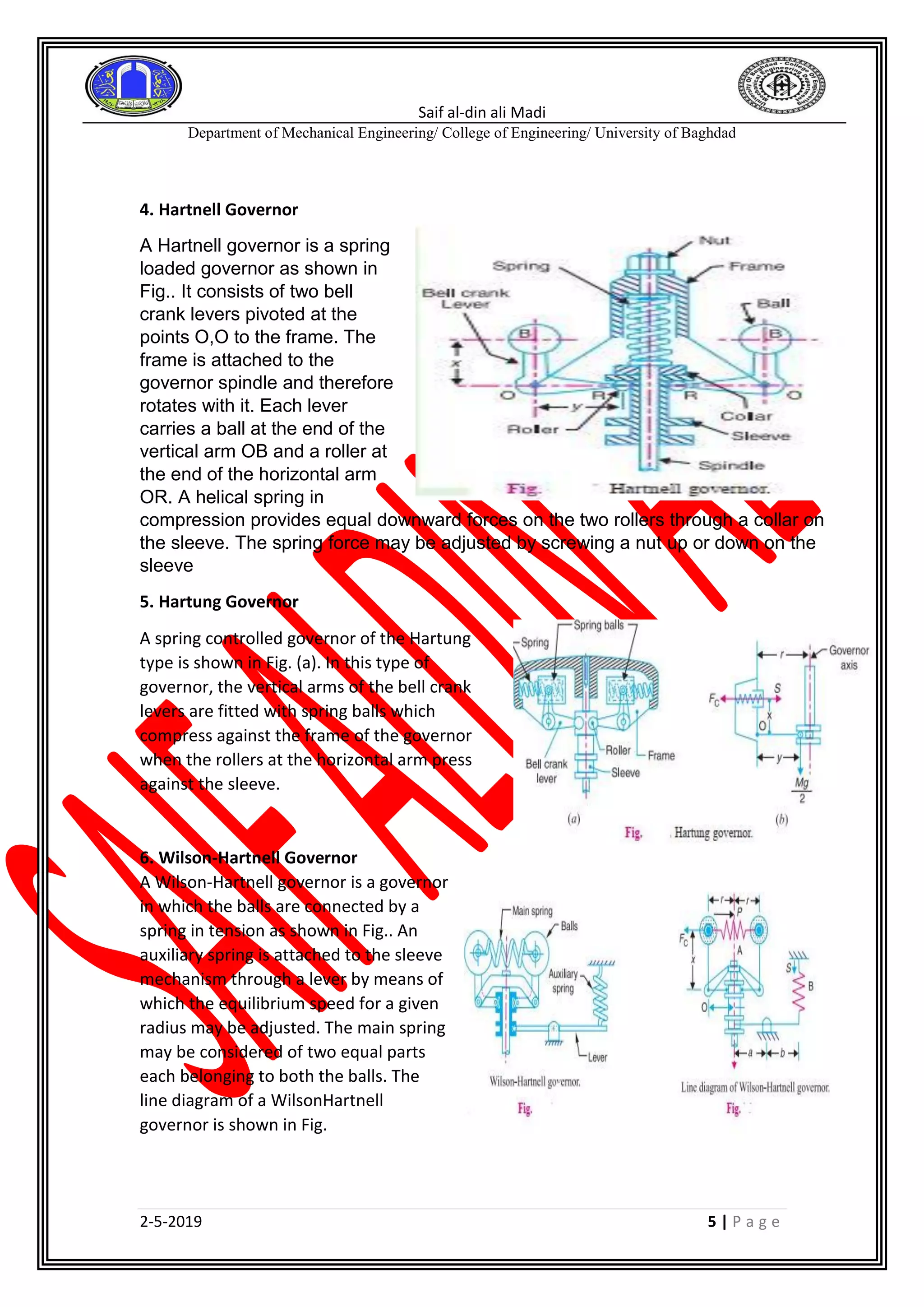
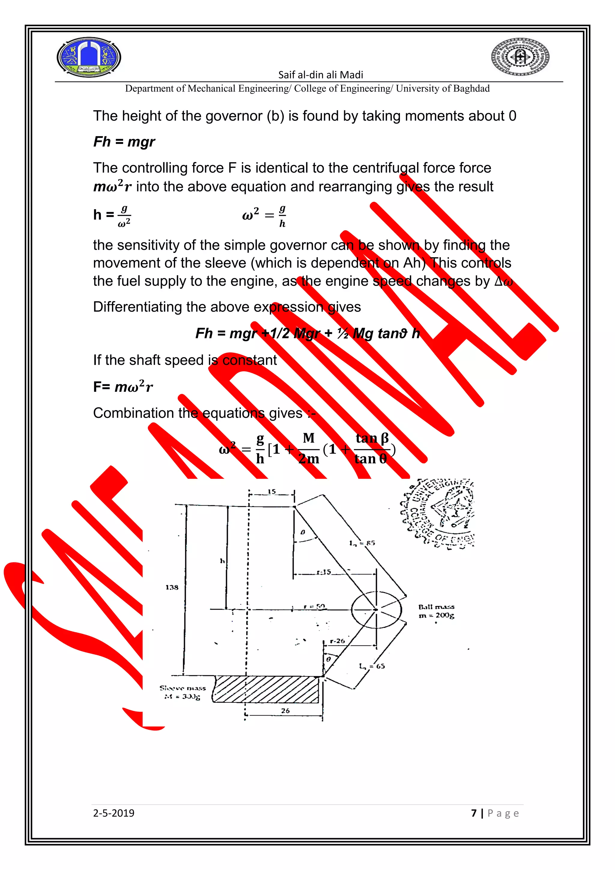
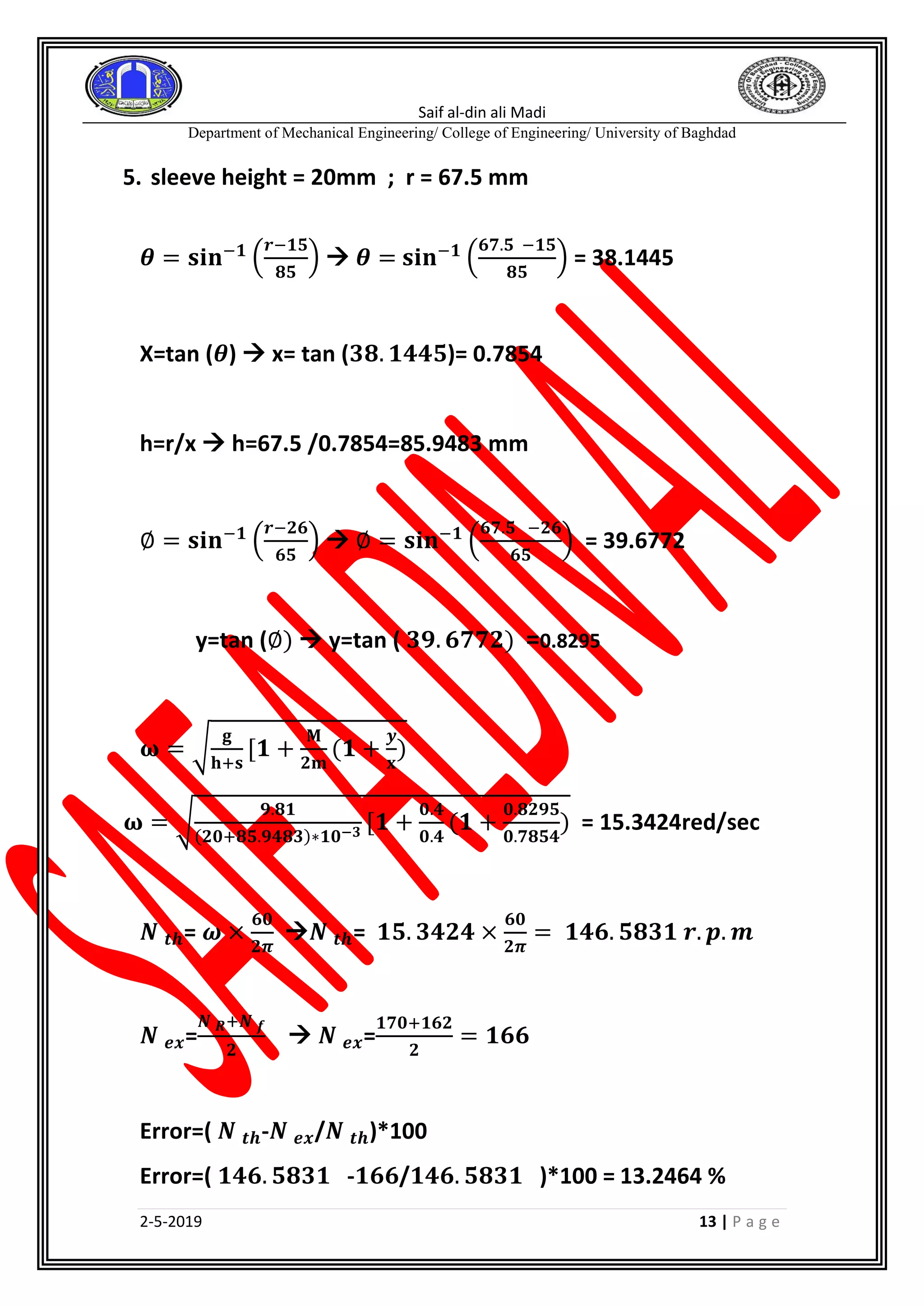
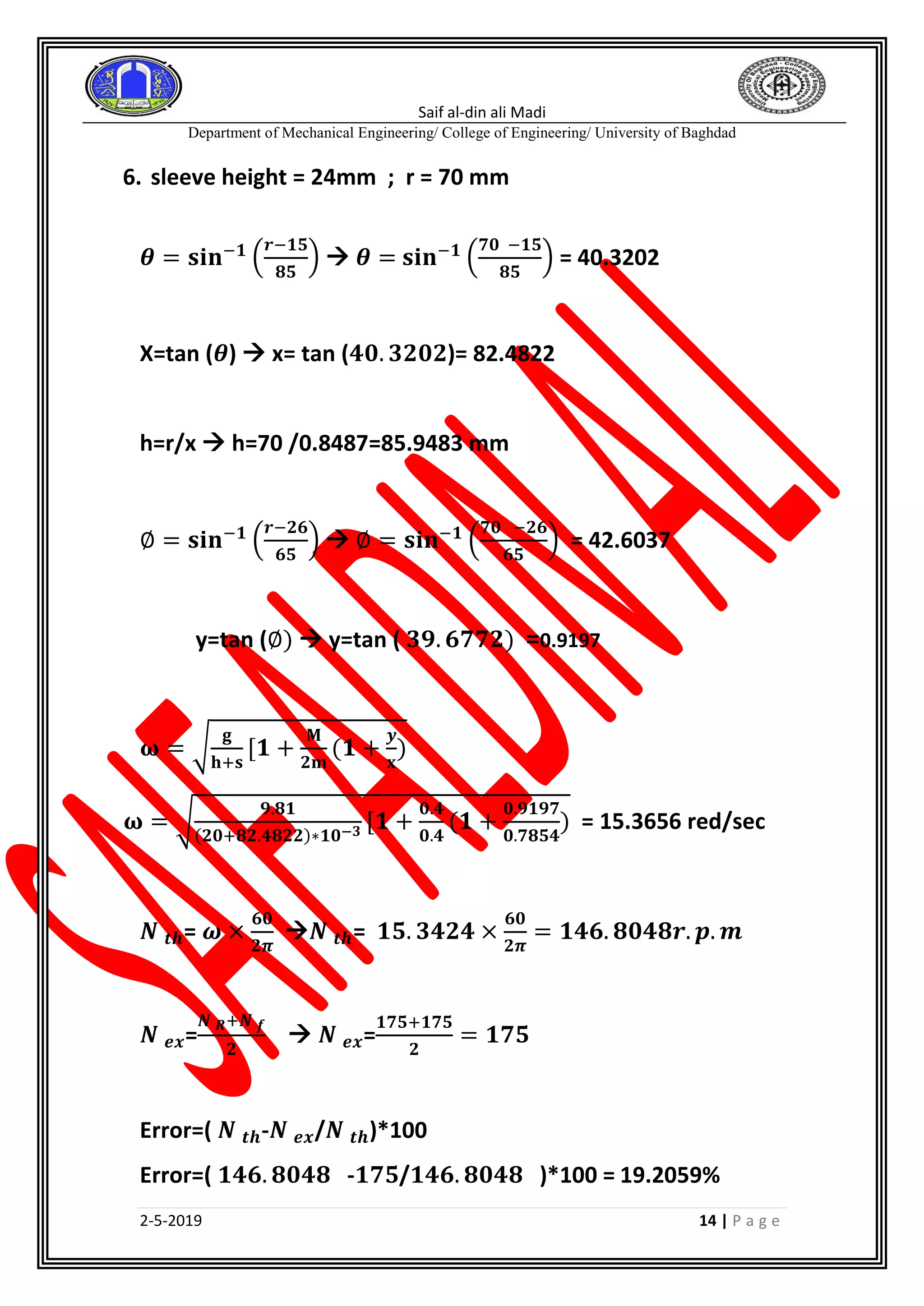
The document outlines a laboratory experiment on the function and characteristics of various governors, specifically focusing on the porter governor. It explains the theory and principles of governors used for speed regulation in engines, along with experimental procedures, calculations, and results obtained from testing different governor configurations. The report includes detailed measurements and analysis of governor performance at various speeds.

1. Saif al-din ali Madi
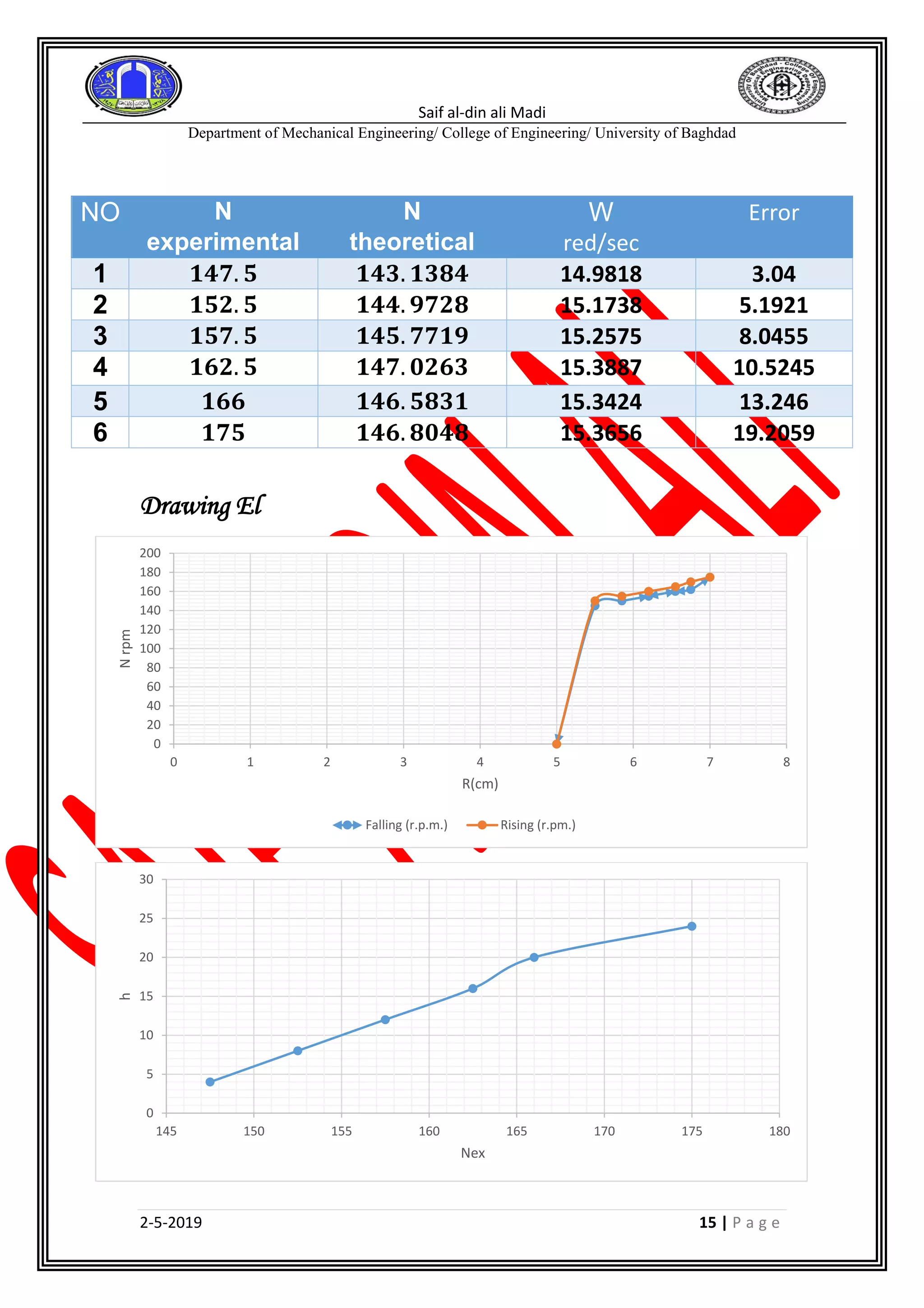
Department of Mechanical Engineering/ College of Engineering/ University of Baghdad
2-5-2019 1 | P a g e
[theory of machine Laboratory II]
University of Baghdad
Name: - Saif Al-din Ali -B-

2. Saif al-din ali Madi
Department of Mechanical Engineering/ College of Engineering/ University of Baghdad
2-5-2019 2 | P a g e
TABLE OF CONTENTS
ABSTRACT.........................................................................I
Objective...........................................................................II
INTRODUCTION...........................................................III
THEORY........................................................................ IV
APPARATUS................................................................. VI
Calculations and results...............................................VII
DISCUSSION ...............................................................VIII

3. Saif al-din ali Madi
Department of Mechanical Engineering/ College of Engineering/ University of Baghdad
2-5-2019 3 | P a g e
Experiment Name:- Governor Apparatus
1. Abstract
The function of a governor is to regulate the mean speed of an engine,
when there are variations in loads e.g. when load on an engine increase
or decrease, obviously its speed will, respectively decrease or increase
to the extent of variation of load. This variation of speed has to be
controlled by the governor, within small limits of mean speed. This
necessitates that when the load increase and consequently the speed
decreases, the supply of fuel to the engine has to be increase
accordingly to compensate for the loss of the speed, so as to bring back
the speed to the mean speed. Conversely, when the load decreases
and speed increases, the supply of fuel has to be reduced
2. OBJECTIVE
To Determine the effect of varying speed on the centre of sleeve in
Porter Governor
3. Introduction
The centrifugal type governors are based on the balancing of centrifugal
force on the rotating balls by an equal and opposite radial force, known
as the controlling force The centrifugal governors are based on the
balancing of centrifugal force on the rotating balls by an equal and
opposite radial force, known as controlling force. In Inertia governors
the position of the balls are affected by the forces set by an angular
acceleration or deceleration of the given spindle in addition to
centrifugal forces on the balls. The apparatus is designed to exhibit the
characteristics of the spring-loaded governor and centrifugal governor.
The experiments shall be performed on following centrifugal type
governors:
1. Watt governor
2. Porter governor
3. Proell governor
4. Hartnell governor

4. Saif al-din ali Madi
Department of Mechanical Engineering/ College of Engineering/ University of Baghdad
2-5-2019 4 | P a g e
1. Watt Governor
The simplest form of a centrifugal governor is a Watt governor, as shown in
Fig. It is basically a conical pendulum with links attached to a sleeve of
negligible mass. The arms of the governor may be connected to the spindle in
the following three ways :
1. The pivot P, may be on the spindle
axis as shown in Fig. (a).
2. The pivot P, may be offset from the
spindle axis and the arms when
produced intersect at O, as shown in
Fig. (b).
3.The pivot P, may be offset, but the
arms cross the axis at O, as shown in
Fig. (c).
2. Porter Governor
The Porter governor is a modification
of a Watt’s governor, with central
load attached to the sleeve as shown
in Fig. (a). The load moves up and
down the central spindle. This
additional downward force increases
the speed of revolution required to
enable the balls to rise to any
predetermined level. Consider the
forces acting on one-half of the
governor as shown in Fig. (b)
3. Proell Governor
The Proell governor has the balls
fixed at B and C to the extension
of the links DF and EG, as shown
in Fig. (a). The arms FP and GQ
are pivoted at P and Q
respectively. Consider the
equilibrium of the forces on one-
half of the governor as shown in
Fig. (b). the instantaneous centre
(I) lies on the intersection of the
line PF produced and the line from D drawn perpendicular to the spindle axis.
The perpendicular BM is drawn on ID.

5. Saif al-din ali Madi
Department of Mechanical Engineering/ College of Engineering/ University of Baghdad
2-5-2019 5 | P a g e
4. Hartnell Governor
A Hartnell governor is a spring
loaded governor as shown in
Fig.. It consists of two bell
crank levers pivoted at the
points O,O to the frame. The
frame is attached to the
governor spindle and therefore
rotates with it. Each lever
carries a ball at the end of the
vertical arm OB and a roller at
the end of the horizontal arm
OR. A helical spring in
compression provides equal downward forces on the two rollers through a collar on
the sleeve. The spring force may be adjusted by screwing a nut up or down on the
sleeve
5. Hartung Governor
A spring controlled governor of the Hartung
type is shown in Fig. (a). In this type of
governor, the vertical arms of the bell crank
levers are fitted with spring balls which
compress against the frame of the governor
when the rollers at the horizontal arm press
against the sleeve.
6. Wilson-Hartnell Governor
A Wilson-Hartnell governor is a governor
in which the balls are connected by a
spring in tension as shown in Fig.. An
auxiliary spring is attached to the sleeve
mechanism through a lever by means of
which the equilibrium speed for a given
radius may be adjusted. The main spring
may be considered of two equal parts
each belonging to both the balls. The
line diagram of a WilsonHartnell
governor is shown in Fig.

6. Saif al-din ali Madi
Department of Mechanical Engineering/ College of Engineering/ University of Baghdad
2-5-2019 6 | P a g e
4. Theory
Governors are used for maintaining the speeds of engines with in
prescribed limits from no load to full load. In petrol engines, the
governor controls the throttle of carburetor and in diesel engines they
control the fuel pump. Most of the governors are of centrifugal type.
These governors use flyweights. Depending upon the speed, the
position of weights change. Which is transmitted to a sleeve through
links. Ultimately the sleeve operates throttle or fuel pump. The
dynamic apparatus consists of a spindle mounted in a vertical position.
Four types of governors can be mounted over the spindle, namely
watt, porter, proell and hartnell. A sleeve attached to governor links is
lifted by outward movement of balls due to centrifugal force. Lift of
sleeve is measured over a scale.
5. APPARATUS
Procedure :-
1. Assemble the governor to be
tested.
2. Complete the electrical
connections.
3. Switch ON the main power.
4. Note down the initial reading of pointer on the scale.
5. Switch On the rotary switch.
6. Slowly increase the speed of governor until the sleeve is lifted
from its initial position by rotating Variac.
7. Let the governor be stabilized.
8. Increase the speed of governor in steps to get the different
positions of sleeve lift at different RPM.
9. Increase the speed of governor in steps to get the different
positions of sleeve lift at different RPM.
Closing Procedure:
Repeat thee processes again with decreasing the speed slowly
Porter Governor

7. Saif al-din ali Madi
Department of Mechanical Engineering/ College of Engineering/ University of Baghdad
2-5-2019 7 | P a g e
The height of the governor (b) is found by taking moments about 0
Fh = mgr
The controlling force F is identical to the centrifugal force force
m𝝎 𝟐
𝒓 into the above equation and rearranging gives the result
h =
𝒈
𝝎 𝟐
𝝎 𝟐
=
𝒈
𝒉
the sensitivity of the simple governor can be shown by finding the
movement of the sleeve (which is dependent on Ah) This controls
the fuel supply to the engine, as the engine speed changes by ∆𝜔
Differentiating the above expression gives
Fh = mgr +1/2 Mgr + ½ Mg tanθ h
If the shaft speed is constant
F= m𝝎 𝟐
𝒓
Combination the equations gives :-
𝛚 𝟐
=
𝐠
𝐡
[𝟏 +
𝐌
𝟐𝐦
(𝟏 +
𝐭𝐚𝐧 𝛃
𝐭𝐚𝐧 𝛉
)

8. Saif al-din ali Madi
Department of Mechanical Engineering/ College of Engineering/ University of Baghdad
2-5-2019 8 | P a g e
Derivation of Porter speed equation
∑ 𝑴𝑰 = 𝟎
Fc* AD -mg ID –
𝑴𝒈
𝟐
∗ 𝑰𝑪 = 𝟎 ÷ 𝑨𝑫
Fc = mg
𝑰𝑫
𝑨𝑫
+
𝑴𝑮
𝟐
∗
𝑰𝑪
𝑨𝑫
= 𝒎𝒈𝐭𝐚 𝐧 𝜽 +
𝑴𝒈
𝟐
(𝐭𝐚 𝐧 𝜽 + 𝐭𝐚 𝐧 𝝋)
Since Fc = m𝝎 𝟐
𝒓
m𝝎 𝟐
𝒓 = mg
𝒓
𝒉
+
𝑴𝒈
𝟐
𝒓
𝒉
( 𝟏 +
𝐭𝐚 𝐧 𝝋
𝐭𝐚 𝐧 𝜽
)
Thus:-
𝛚 𝟐
=
𝐠
𝐡
[𝟏 +
𝐌
𝟐𝐦
(𝟏 +
𝐭𝐚𝐧 𝛃
𝐭𝐚𝐧 𝛉
)
Proell Governor
ThePROELL governor is similar to the Porter governor
except that the governor ball balls fixed to extensions of the links,
as shown in Figure 3. The arm reacts shaft pivot with a force T1.
As with the Porter governor, the reaction of the link on t sleeve
(T2) can be resolved into a vertical component ½ Mg and a
horizontal component H.
Ti and H need not be calculated if moments are taken about the
Point O
𝑭 𝒀 = 𝒎𝒈(𝒙 − 𝒓) +
𝟏
𝟐
𝑴𝒈(𝒙 − 𝒃)
Also, if the shaft speed is steady. F is given by Equation 2.5
F=m𝝎 𝟐
𝒓
An expression for co as a function of y can be found by combining
Equations 2.5 and 2.9. Hences
𝝎 𝟐
= [(𝒙 − 𝒓) +
𝑴
𝟐𝒎
(𝒙 − 𝒃)] ×
𝒈
𝒚. 𝒓

9. Saif al-din ali Madi
Department of Mechanical Engineering/ College of Engineering/ University of Baghdad
2-5-2019 9 | P a g e
6. Calculations and results
1. sleeve height = 4 mm ; r = 55 mm
𝜽 = 𝐬𝐢𝐧−𝟏
(
𝒓−𝟏𝟓
𝟖𝟓
)  𝜽 = 𝐬𝐢𝐧−𝟏
(
𝟓𝟓−𝟏𝟓
𝟖𝟓
) = 28.0725
X=tan (𝜽)  x= tan (𝟐𝟖. 𝟎𝟕𝟐𝟓) = 0.5333
h=r/x  h=55/0.5333 = 103.1250 mm
∅ = 𝐬𝐢𝐧−𝟏
(
𝒓−𝟐𝟔
𝟔𝟓
)  ∅ = 𝐬𝐢𝐧−𝟏
(
𝟓𝟓−𝟐𝟔
𝟔𝟓
) =26.4972
y=tan (∅)  y=tan (𝟐𝟔. 𝟒𝟗𝟕𝟐) = 0.4985
𝛚 = √
𝐠
𝐡+𝐬
[𝟏 +
𝐌
𝟐𝐦
(𝟏 +
𝒚
𝐱
)
𝛚 = √
𝟗.𝟖𝟏
(𝟒+𝟏𝟎𝟑.𝟏)∗𝟏𝟎−𝟑 [𝟏 +
𝟎.𝟒
𝟎.𝟒
(𝟏 +
𝟎.𝟒𝟗𝟖𝟓
𝟎.𝟓𝟑𝟑𝟑
) =14.9818 red/sec
𝑵 𝒕𝒉= 𝝎 ×
𝟔𝟎
𝟐𝝅
𝑵 𝒕𝒉= 𝟏𝟒. 𝟗𝟖𝟏𝟖 ×
𝟔𝟎
𝟐𝝅
= 𝟏𝟒𝟑. 𝟏𝟑𝟖𝟒 𝒓. 𝒑. 𝒎
𝑵 𝒆𝒙=
𝑵 𝑹+𝑵 𝒇
𝟐
 𝑵 𝒆𝒙=
𝟏𝟓𝟎+𝟏𝟒𝟓
𝟐
= 𝟏𝟒𝟕. 𝟓
Error=( 𝑵 𝒕𝒉-𝑵 𝒆𝒙/𝑵 𝒕𝒉)*100
Error=( 𝟏𝟒𝟑. 𝟏𝟑𝟖𝟒 -𝟏𝟒𝟕. 𝟓 /𝟏𝟒𝟑. 𝟏𝟑𝟖𝟒 )*100 =3.04%
NO h(mm) Rising (r.pm.) Falling (r.p.m.) R(cm)
0 0 0 0 5
1 4 150 145 5.5
2 8 155 150 5.85
3 12 160 155 6.2
4 16 165 160 6.55
5 20 170 162 6.75
6 24 175 175 7

10. Saif al-din ali Madi
Department of Mechanical Engineering/ College of Engineering/ University of Baghdad
2-5-2019 10 | P a g e
2. sleeve height = 8 mm ; r = 58.9 mm
𝜽 = 𝐬𝐢𝐧−𝟏
(
𝒓−𝟏𝟓
𝟖𝟓
)  𝜽 = 𝐬𝐢𝐧−𝟏
(
𝟓𝟖.𝟗 −𝟏𝟓
𝟖𝟓
) = 31.0958
X=tan (𝜽)  x= tan (𝟑𝟏. 𝟎𝟗𝟓𝟖) = 0.6031
h=r/x  h=58.9 /0.6031=97.6558 mm
∅ = 𝐬𝐢𝐧−𝟏
(
𝒓−𝟐𝟔
𝟔𝟓
)  ∅ = 𝐬𝐢𝐧−𝟏
(
𝟓𝟖.𝟗 −𝟐𝟔
𝟔𝟓
) = 30.4080
y=tan (∅)  y=tan ( 𝟑𝟎. 𝟒𝟎𝟖𝟎) =0.58969
𝛚 = √
𝐠
𝐡+𝐬
[𝟏 +
𝐌
𝟐𝐦
(𝟏 +
𝒚
𝐱
)
𝛚 = √
𝟗.𝟖𝟏
(𝟖+𝟗𝟕.𝟔𝟓𝟓𝟖)∗𝟏𝟎−𝟑 [𝟏 +
𝟎.𝟒
𝟎.𝟒
(𝟏 +
𝟎.𝟓𝟖𝟗𝟔𝟗
𝟎.𝟔𝟎𝟑𝟏
) =15.1738red/sec
𝑵 𝒕𝒉= 𝝎 ×
𝟔𝟎
𝟐𝝅
𝑵 𝒕𝒉= 𝟏𝟓. 𝟏𝟕𝟑𝟖 ×
𝟔𝟎
𝟐𝝅
= 𝟏𝟒𝟒. 𝟗𝟕𝟐𝟖 𝒓. 𝒑. 𝒎
𝑵 𝒆𝒙=
𝑵 𝑹+𝑵 𝒇
𝟐
 𝑵 𝒆𝒙=
𝟏𝟓𝟎+𝟏𝟓𝟓
𝟐
= 𝟏𝟓𝟐. 𝟓𝟎𝟎𝟎
Error=( 𝑵 𝒕𝒉-𝑵 𝒆𝒙/𝑵 𝒕𝒉)*100
Error=( 𝟏𝟒𝟒. 𝟗𝟕𝟐𝟖 -𝟏𝟓𝟐. 𝟓𝟎𝟎𝟎 /𝟏𝟒𝟒. 𝟗𝟕𝟐𝟖 )*100 = 5.1921 %

11. Saif al-din ali Madi
Department of Mechanical Engineering/ College of Engineering/ University of Baghdad
2-5-2019 11 | P a g e
3. sleeve height = 12 mm ; r = 62 mm
𝜽 = 𝐬𝐢𝐧−𝟏
(
𝒓−𝟏𝟓
𝟖𝟓
)  𝜽 = 𝐬𝐢𝐧−𝟏
(
𝟔𝟐 −𝟏𝟓
𝟖𝟓
) = 33.5690
X=tan (𝜽)  x= tan (𝟑𝟑. 𝟓𝟔𝟗𝟎) = 0.6636
h=r/x  h=62 /0.6636=93.4270mm
∅ = 𝐬𝐢𝐧−𝟏
(
𝒓−𝟐𝟔
𝟔𝟓
)  ∅ = 𝐬𝐢𝐧−𝟏
(
𝟔𝟐 −𝟐𝟔
𝟔𝟓
) = 33.6313
y=tan (∅)  y=tan ( 𝟑𝟑. 𝟔𝟑𝟏𝟑) =0.6652
𝛚 = √
𝐠
𝐡+𝐬
[𝟏 +
𝐌
𝟐𝐦
(𝟏 +
𝒚
𝐱
)
𝛚 = √
𝟗.𝟖𝟏
(𝟏𝟐+𝟗𝟑.𝟒𝟐𝟕𝟎)∗𝟏𝟎−𝟑 [𝟏 +
𝟎.𝟒
𝟎.𝟒
(𝟏 +
𝟎.𝟔𝟔𝟓𝟐
𝟎.𝟔𝟔𝟑𝟔
) =15.2575 red/sec
𝑵 𝒕𝒉= 𝝎 ×
𝟔𝟎
𝟐𝝅
𝑵 𝒕𝒉= 𝟏𝟓. 𝟐𝟓𝟕𝟓 ×
𝟔𝟎
𝟐𝝅
= 𝟏𝟒𝟓. 𝟕𝟕𝟏𝟗𝒓. 𝒑. 𝒎
𝑵 𝒆𝒙=
𝑵 𝑹+𝑵 𝒇
𝟐
 𝑵 𝒆𝒙=
𝟏𝟔𝟎+𝟏𝟓𝟓
𝟐
= 𝟏𝟓𝟕. 𝟓
Error=( 𝑵 𝒕𝒉-𝑵 𝒆𝒙/𝑵 𝒕𝒉)*100
Error=( 𝟏𝟒𝟓. 𝟕𝟕 -𝟏𝟓𝟕. 𝟓 /𝟏𝟒𝟓. 𝟕𝟕 )*100 =8.0455%

12. Saif al-din ali Madi
Department of Mechanical Engineering/ College of Engineering/ University of Baghdad
2-5-2019 12 | P a g e
4. sleeve height = 16mm ; r = 65.5 mm
𝜽 = 𝐬𝐢𝐧−𝟏
(
𝒓−𝟏𝟓
𝟖𝟓
)  𝜽 = 𝐬𝐢𝐧−𝟏
(
𝟔𝟓.𝟓 −𝟏𝟓
𝟖𝟓
) = 36.4498
X=tan (𝜽)  x= tan (𝟑𝟔. 𝟒𝟒𝟗𝟖)= 0.7386
h=r/x  h=65.5 /0.7386=88.6807 mm
∅ = 𝐬𝐢𝐧−𝟏
(
𝒓−𝟐𝟔
𝟔𝟓
)  ∅ = 𝐬𝐢𝐧−𝟏
(
𝟔𝟓.𝟓 −𝟐𝟔
𝟔𝟓
) = 37.4228
y=tan (∅)  y=tan ( 𝟑𝟕. 𝟒𝟐𝟐𝟖) =0.7652
𝛚 = √
𝐠
𝐡+𝐬
[𝟏 +
𝐌
𝟐𝐦
(𝟏 +
𝒚
𝐱
)
𝛚 = √
𝟗.𝟖𝟏
(𝟏𝟔+𝟖𝟖.𝟔𝟖𝟎𝟕)∗𝟏𝟎−𝟑 [𝟏 +
𝟎.𝟒
𝟎.𝟒
(𝟏 +
𝟎.𝟕𝟔𝟓𝟐
𝟎.𝟕𝟑𝟖𝟔
) =15.3887 red/sec
𝑵 𝒕𝒉= 𝝎 ×
𝟔𝟎
𝟐𝝅
𝑵 𝒕𝒉= 𝟏𝟓. 𝟑𝟖𝟖𝟕 ×
𝟔𝟎
𝟐𝝅
= 𝟏𝟒𝟕. 𝟎𝟐𝟔𝟑 𝒓. 𝒑. 𝒎
𝑵 𝒆𝒙=
𝑵 𝑹+𝑵 𝒇
𝟐
 𝑵 𝒆𝒙=
𝟏𝟔𝟎+𝟏𝟔𝟓
𝟐
= 𝟏𝟔𝟐. 𝟓
Error=( 𝑵 𝒕𝒉-𝑵 𝒆𝒙/𝑵 𝒕𝒉)*100
Error=( 𝟏𝟒𝟕. 𝟎𝟐𝟔𝟑 -𝟏𝟔𝟐. 𝟓/𝟏𝟒𝟕. 𝟎𝟐𝟔𝟑 )*100 = 10.5245 %

13. Saif al-din ali Madi
Department of Mechanical Engineering/ College of Engineering/ University of Baghdad
2-5-2019 13 | P a g e
5. sleeve height = 20mm ; r = 67.5 mm
𝜽 = 𝐬𝐢𝐧−𝟏
(
𝒓−𝟏𝟓
𝟖𝟓
)  𝜽 = 𝐬𝐢𝐧−𝟏
(
𝟔𝟕.𝟓 −𝟏𝟓
𝟖𝟓
) = 38.1445
X=tan (𝜽)  x= tan (𝟑𝟖. 𝟏𝟒𝟒𝟓)= 0.7854
h=r/x  h=67.5 /0.7854=85.9483 mm
∅ = 𝐬𝐢𝐧−𝟏
(
𝒓−𝟐𝟔
𝟔𝟓
)  ∅ = 𝐬𝐢𝐧−𝟏
(
𝟔𝟕.𝟓 −𝟐𝟔
𝟔𝟓
) = 39.6772
y=tan (∅)  y=tan ( 𝟑𝟗. 𝟔𝟕𝟕𝟐) =0.8295
𝛚 = √
𝐠
𝐡+𝐬
[𝟏 +
𝐌
𝟐𝐦
(𝟏 +
𝒚
𝐱
)
𝛚 = √
𝟗.𝟖𝟏
(𝟐𝟎+𝟖𝟓.𝟗𝟒𝟖𝟑)∗𝟏𝟎−𝟑 [𝟏 +
𝟎.𝟒
𝟎.𝟒
(𝟏 +
𝟎.𝟖𝟐𝟗𝟓
𝟎.𝟕𝟖𝟓𝟒
) = 15.3424red/sec
𝑵 𝒕𝒉= 𝝎 ×
𝟔𝟎
𝟐𝝅
𝑵 𝒕𝒉= 𝟏𝟓. 𝟑𝟒𝟐𝟒 ×
𝟔𝟎
𝟐𝝅
= 𝟏𝟒𝟔. 𝟓𝟖𝟑𝟏 𝒓. 𝒑. 𝒎
𝑵 𝒆𝒙=
𝑵 𝑹+𝑵 𝒇
𝟐
 𝑵 𝒆𝒙=
𝟏𝟕𝟎+𝟏𝟔𝟐
𝟐
= 𝟏𝟔𝟔
Error=( 𝑵 𝒕𝒉-𝑵 𝒆𝒙/𝑵 𝒕𝒉)*100
Error=( 𝟏𝟒𝟔. 𝟓𝟖𝟑𝟏 -𝟏𝟔𝟔/𝟏𝟒𝟔. 𝟓𝟖𝟑𝟏 )*100 = 13.2464 %

14. Saif al-din ali Madi
Department of Mechanical Engineering/ College of Engineering/ University of Baghdad
2-5-2019 14 | P a g e
6. sleeve height = 24mm ; r = 70 mm
𝜽 = 𝐬𝐢𝐧−𝟏
(
𝒓−𝟏𝟓
𝟖𝟓
)  𝜽 = 𝐬𝐢𝐧−𝟏
(
𝟕𝟎 −𝟏𝟓
𝟖𝟓
) = 40.3202
X=tan (𝜽)  x= tan (𝟒𝟎. 𝟑𝟐𝟎𝟐)= 82.4822
h=r/x  h=70 /0.8487=85.9483 mm
∅ = 𝐬𝐢𝐧−𝟏
(
𝒓−𝟐𝟔
𝟔𝟓
)  ∅ = 𝐬𝐢𝐧−𝟏
(
𝟕𝟎 −𝟐𝟔
𝟔𝟓
) = 42.6037
y=tan (∅)  y=tan ( 𝟑𝟗. 𝟔𝟕𝟕𝟐) =0.9197
𝛚 = √
𝐠
𝐡+𝐬
[𝟏 +
𝐌
𝟐𝐦
(𝟏 +
𝒚
𝐱
)
𝛚 = √
𝟗.𝟖𝟏
(𝟐𝟎+𝟖𝟐.𝟒𝟖𝟐𝟐)∗𝟏𝟎−𝟑 [𝟏 +
𝟎.𝟒
𝟎.𝟒
(𝟏 +
𝟎.𝟗𝟏𝟗𝟕
𝟎.𝟕𝟖𝟓𝟒
) = 15.3656 red/sec
𝑵 𝒕𝒉= 𝝎 ×
𝟔𝟎
𝟐𝝅
𝑵 𝒕𝒉= 𝟏𝟓. 𝟑𝟒𝟐𝟒 ×
𝟔𝟎
𝟐𝝅
= 𝟏𝟒𝟔. 𝟖𝟎𝟒𝟖𝒓. 𝒑. 𝒎
𝑵 𝒆𝒙=
𝑵 𝑹+𝑵 𝒇
𝟐
 𝑵 𝒆𝒙=
𝟏𝟕𝟓+𝟏𝟕𝟓
𝟐
= 𝟏𝟕𝟓
Error=( 𝑵 𝒕𝒉-𝑵 𝒆𝒙/𝑵 𝒕𝒉)*100
Error=( 𝟏𝟒𝟔. 𝟖𝟎𝟒𝟖 -𝟏𝟕𝟓/𝟏𝟒𝟔. 𝟖𝟎𝟒𝟖 )*100 = 19.2059%

15. Saif al-din ali Madi
Department of Mechanical Engineering/ College of Engineering/ University of Baghdad
2-5-2019 15 | P a g e
Drawing El
0
20
40
60
80
100
120
140
160
180
200
0 1 2 3 4 5 6 7 8
Nrpm
R(cm)
Falling (r.p.m.) Rising (r.pm.)
0
5
10
15
20
25
30
145 150 155 160 165 170 175 180
h
Nex
NO N
experimental
N
theoretical
W
red/sec
Error
1 𝟏𝟒𝟕. 𝟓 𝟏𝟒𝟑. 𝟏𝟑𝟖𝟒 14.9818 3.04
2 𝟏𝟓𝟐. 𝟓 𝟏𝟒𝟒. 𝟗𝟕𝟐𝟖 15.1738 5.1921
3 𝟏𝟓𝟕. 𝟓 𝟏𝟒𝟓. 𝟕𝟕𝟏𝟗 15.2575 8.0455
4 𝟏𝟔𝟐. 𝟓 𝟏𝟒𝟕. 𝟎𝟐𝟔𝟑 15.3887 10.5245
5 𝟏𝟔𝟔 𝟏𝟒𝟔. 𝟓𝟖𝟑𝟏 15.3424 13.246
6 𝟏𝟕𝟓 𝟏𝟒𝟔. 𝟖𝟎𝟒𝟖 15.3656 19.2059