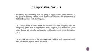
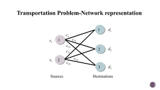
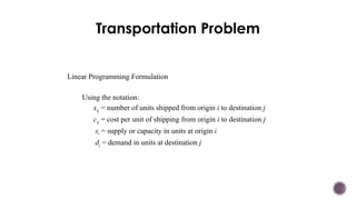
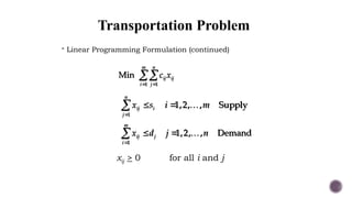
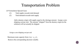
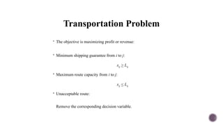
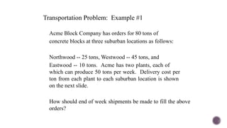
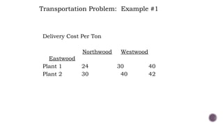
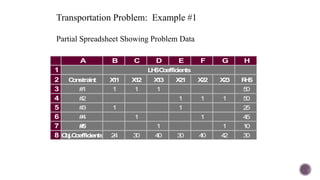
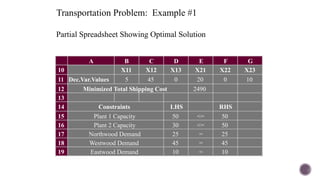
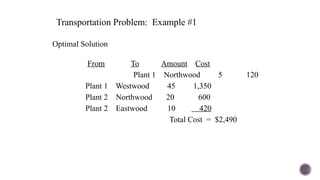
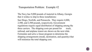
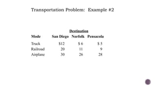
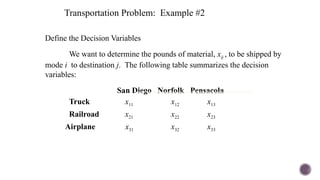
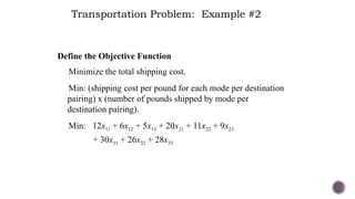
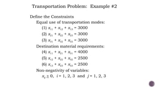
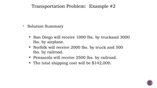
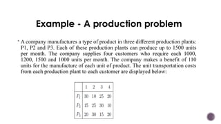
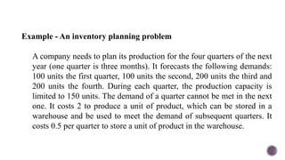
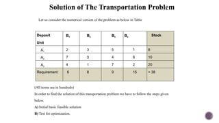
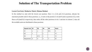
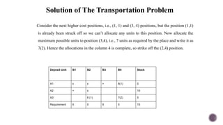
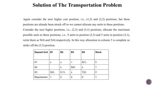
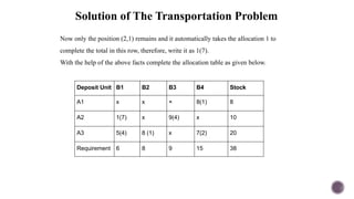
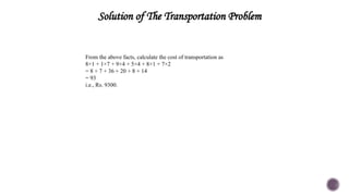
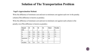
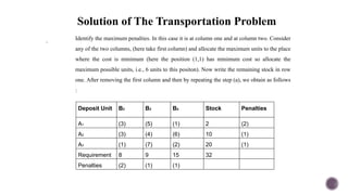
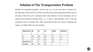
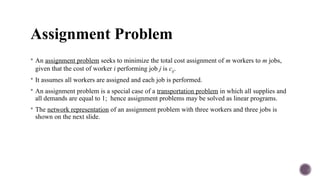
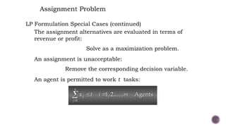
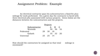
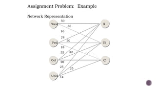
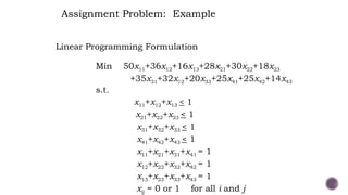
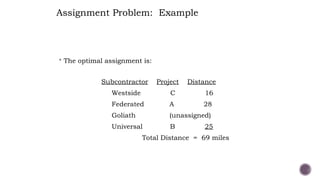
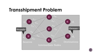
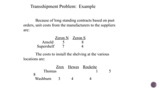
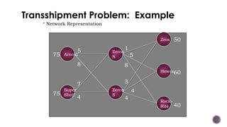
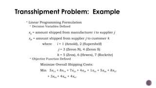
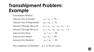
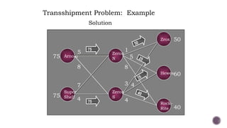
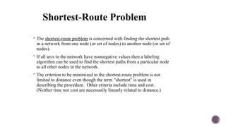
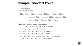
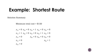
Transportation, Transshipment and Assignment Problem.pptx

Transportation, and
Assignment Problem
Kiran Garg

Network Models
 A network model is one which can be represented by a set of nodes, a
set of arcs, and functions (e.g. costs, supplies, demands, etc.)
associated with the arcs and/or nodes.
 Transportation, assignment, transshipment, shortest-route, and
maximal flow problems of this chapter as well as the minimal
spanning tree and PERT/CPM problems (in others chapter) are all
examples of network problems.

Network Models
 Each of the five problems of this chapter can be formulated as linear
programs and solved by general purpose linear programming codes.
 For each of the five problems, if the right-hand side of the linear
programming formulations are all integers, the optimal solution will be
in terms of integer values for the decision variables.
 However, there are many computer packages that contain separate
computer codes for these problems which take advantage of their
network structure.

Transportation Problem
 Distributing any commodity from any group of supply centers, called sources, to
any group of receiving centers, called destinations, in such a way as to minimize
the total distribution cost (shipping cost).
 The transportation problem seeks to minimize the total shipping costs of
transporting goods from m origins (each with a supply si) to n destinations (each
with a demand dj), when the unit shipping cost from an origin, i, to a destination,
j, is cij.
 The network representation for a transportation problem with two sources and
three destinations is given on the next slide.

Transportation Problem-Network representation
2
c1
c12
c13
c21
c22
c23
d1
d2
d3
s1
s2
Sources Destinations
3
2
1
1

Linear Programming Formulation
Using the notation:
xij = number of units shipped from origin i to destination j
cij = cost per unit of shipping from origin i to destination j
si = supply or capacity in units at origin i
dj = demand in units at destination j

 Linear Programming Formulation (continued)
 

1 1
Min
m n
ij ij
i j
c x

 
 
1
1,2, , Supply
n
ij i
j
x s i m

 
 
1
1,2, , Demand
m
ij j
i
x d j n
xij > 0 for all i and j

LP Formulation Special Cases
(1) Total supply exceeds total demand
(2) Total demand exceeds total supply
Add a dummy origin with supply equal to the shortage amount. Assign a zero
shipping cost per unit. The amount “shipped” from the dummy origin (in the
solution) will not actually be shipped.
Assign a zero shipping cost per unit
Maximum route capacity from i to j: xij < Li
Remove the corresponding decision variable.

 The objective is maximizing profit or revenue:
 Minimum shipping guarantee from i to j:
xij > Lij
 Maximum route capacity from i to j:
xij < Lij
 Unacceptable route:

Transportation Problem: Example #1
Acme Block Company has orders for 80 tons of
concrete blocks at three suburban locations as follows:
Northwood -- 25 tons, Westwood -- 45 tons, and
Eastwood -- 10 tons. Acme has two plants, each of
which can produce 50 tons per week. Delivery cost per
ton from each plant to each suburban location is shown
on the next slide.
How should end of week shipments be made to fill the above
orders?

Delivery Cost Per Ton
Northwood Westwood
Eastwood
Plant 1 24 30 40
Plant 2 30 40 42

Partial Spreadsheet Showing Problem Data
A B C D E F G H
1
2 C
o
n
stra
in
t X
1
1 X
1
2 X
1
3 X
2
1 X
2
2 X
2
3 R
H
S
3 #
1 1 1 1 5
0
4 #
2 1 1 1 5
0
5 #
3 1 1 2
5
6 #
4 1 1 4
5
7 #
5 1 1 1
0
8 O
b
j.C
o
effic
ien
ts 2
4 3
0 4
0 3
0 4
0 4
2 3
0
L
H
SC
o
effic
ien
ts

A B C D E F G
10 X11 X12 X13 X21 X22 X23
11 Dec.Var.Values 5 45 0 20 0 10
12 Minimized Total Shipping Cost 2490
13
14 LHS RHS
15 50 <= 50
16 30 <= 50
17 25 = 25
18 45 = 45
19 10 = 10
Eastwood Demand
Westwood Demand
Northwood Demand
Constraints
Plant 1 Capacity
Plant 2 Capacity
Partial Spreadsheet Showing Optimal Solution

Optimal Solution
From To Amount Cost
Plant 1 Northwood 5 120
Plant 1 Westwood 45 1,350
Plant 2 Northwood 20 600
Plant 2 Eastwood 10 420
Total Cost = $2,490

The Navy has 9,000 pounds of material in Albany, Georgia
that it wishes to ship to three installations:
San Diego, Norfolk, and Pensacola. They require 4,000,
2,500, and 2,500 pounds, respectively. Government
regulations require equal distribution of shipping among the
three carriers. The shipping costs per pound for truck,
railroad, and airplane transit are shown on the next slide.
Formulate and solve a linear program to determine the
shipping arrangements (mode, destination, and quantity) that
will minimize the total shipping cost.

Destination
Mode San Diego Norfolk Pensacola
Truck $12 $ 6 $ 5
Railroad 20 11 9
Airplane 30 26 28

Define the Decision Variables
We want to determine the pounds of material, xij , to be shipped by
mode i to destination j. The following table summarizes the decision
variables:
San Diego Norfolk Pensacola
Truck x11 x12 x13
Railroad x21 x22 x23
Airplane x31 x32 x33

Define the Objective Function
Minimize the total shipping cost.
Min: (shipping cost per pound for each mode per destination
pairing) x (number of pounds shipped by mode per
destination pairing).
Min: 12x11 + 6x12 + 5x13 + 20x21 + 11x22 + 9x23
+ 30x31 + 26x32 + 28x33

Define the Constraints
Equal use of transportation modes:
(1) x11 + x12 + x13 = 3000
(2) x21 + x22 + x23 = 3000
(3) x31 + x32 + x33 = 3000
Destination material requirements:
(4) x11 + x21 + x31 = 4000
(5) x12 + x22 + x32 = 2500
(6) x13 + x23 + x33 = 2500
Non-negativity of variables:
xij > 0, i = 1, 2, 3 and j = 1, 2, 3

• Solution Summary
• San Diego will receive 1000 lbs. by truckand 3000
lbs. by airplane.
• Norfolk will receive 2000 lbs. by truck and 500
lbs. by railroad.
• Pensacola will receive 2500 lbs. by railroad.
• The total shipping cost will be $142,000.

Example - A production problem
 A company manufactures a type of product in three different production plants:
P1, P2 and P3. Each of these production plants can produce up to 1500 units
per month. The company supplies four customers who require each 1000,
1200, 1500 and 1000 units per month. The company makes a benefit of 110
units for the manufacture of each unit of product. The unit transportation costs
from each production plant to each customer are displayed below:

Example - An inventory planning problem
A company needs to plan its production for the four quarters of the next
year (one quarter is three months). It forecasts the following demands:
100 units the first quarter, 100 units the second, 200 units the third and
200 units the fourth. During each quarter, the production capacity is
limited to 150 units. The demand of a quarter cannot be met in the next
one. It costs 2 to produce a unit of product, which can be stored in a
warehouse and be used to meet the demand of subsequent quarters. It
costs 0.5 per quarter to store a unit of product in the warehouse.

Finding an initial basic feasible solution
The procedure of calculating an initial basic feasible
solution is performed in a tableau of the same
dimensions as the transportation costs tableau; the
transportation solution tableau, where each position
(i, j) is associated with the decision variable xij , that
is, the number of units of product to be transported
from origin Oi to destination Dj. Such positions (i, j)
are called cells, and represent a solution. An empty
cell denotes a value of zero.

Solution of The Transportation Problem
Let us consider the numerical version of the problem as below in Table
Deposit
Unit
B1 B2 B3 B4
Stock
A1
2 3 5 1 8
A2
7 3 4 6 10
A3
4 1 7 2 20
Requirement 6 8 9 15 = 38
(All terms are in hundreds)
In order to find the solution of this transportation problem we have to follow the steps given
below.
A) Initial basic feasible solution
B) Test for optimization.

Lowest Cost Entry Method or Matrix Minima Method:
In this method we start with the lowest cost position. Here it is (1,4) and (3,2) positions, allocate the
maximum possible units to these positions, i.e., 8 units to the position (1,4) and 8 units to position (3,2), write
them as 8(1)and 8(1) respectively, then strike off the other positions in row 1 and also in column 2, since all
the available units are distributed to these positions.
Deposit Unit B1 B2 B3 B4 Stock
A1 x x × 8(1) 8
A2 × x 10
A3 8 (1) x 12
Requirement 6 0 9 7 22

Consider the next higher cost positions, i.e., (1, 1) and (3, 4) positions, but the position (1,1)
is already been struck off so we can’t allocate any units to this position. Now allocate the
maximum possible units to position (3,4), i.e., 7 units as required by the place and write it as
7(2). Hence the allocations in the column 4 is complete, so strike off the (2,4) position.
A1 x x × 8(1) 0
A2 × x 10
A3 8 (1) 7(2) 5

Again consider the next higher cost position, i.e., (1,2) and (2,2) positions, but these
positions are already been struck off so we cannot allocate any units to these positions.
Consider the next higher positions, i.e., (2,3) and (3,1) positions, allocate the maximum
possible units to these positions, i.e., 9 units to position (2,3) and 5 units to position (3,1),
write them as 9(4) and 5(4) respectively. In this way allocation in column 3 is complete so
strike off the (3,3) position.
A1 x x × 8(1) 0
A2 x 9(4) x 1
A3 5(4) 8 (1) x 7(2) 0

Now only the position (2,1) remains and it automatically takes the allocation 1 to
complete the total in this row, therefore, write it as 1(7).
With the help of the above facts complete the allocation table as given below.
A1 x x × 8(1) 8
A2 1(7) x 9(4) x 10
A3 5(4) 8 (1) x 7(2) 20

From the above facts, calculate the cost of transportation as
8×1 + 1×7 + 9×4 + 5×4 + 8×1 + 7×2
= 8 + 7 + 36 + 20 + 8 + 14
= 93
i.e., Rs. 9300.

Vogel’s Approximation Method:
Write the difference of minimum cost and next to minimum cost against each row in the penalty
column.(This difference is known as penalty).
Write the difference of minimum cost and next to minimum cost against each column in the
penalty row.(This difference is known as penalty).
Deposit
Unit
B1 B2 B3 B4 Stock Penaltie
s
A1 (2) (3) (5) (1) 8 (1)
A2 (7) (3) (4) (6) 10 (1)
A3 (4) (1) (7) (2) 20 (1)
Requireme
nt
6 8 9 15 38
Penalties (2) (2) (1) (1)

.
Identify the maximum penalties. In this case it is at column one and at column two. Consider
any of the two columns, (here take first column) and allocate the maximum units to the place
where the cost is minimum (here the position (1,1) has minimum cost so allocate the
maximum possible units, i.e., 6 units to this positon). Now write the remaining stock in row
one. After removing the first column and then by repeating the step (a), we obtain as follows
:
Deposit Unit B2 B3 B4 Stock Penalties
A1 (3) (5) (1) 2 (2)
A2 (3) (4) (6) 10 (1)
A3 (1) (7) (2) 20 (1)
Requirement 8 9 15 32
Penalties (2) (1) (1)

Identify the maximum penalties. In this case it is at row one and at column two.
Consider any of the two (let it be first row) and allocate the maximum possible units to
the place where the cost is minimum (here the position (1,4) has minimum cost so
allocate the maximum possible units, i.e., 2 units to this position). Now write the
remaining stock in column four. After removing the first row and by repeating the
step(a), we obtain table 14 as given below :
Deposit Unit B2 B3 B4 Stock Penalties
A2 (3) (4) (6) 10 (1)
A3 (1) (7) (2) 20 (1)
Requirement 8 9 13 32
Penalties (2) (3) (4)

Solution of The Transportation
Problem
Identify the maximum penalties. In this case it is at column four. Now allocate the maximum
possible units to the minimum cost position (here it is at (3,4) position and allocate maximum
possible units, i.e., 13 to this positon). Now write the remaining stock in row three. After
removing the fourth column and then by repeating the step (a) we obtain table 15 as given below.
Deposit Unit B2 B3 Stock Penalties
A2 (3) (4) 10 (1)
A3 (1) (7) 7 (6)
Requirement 8 9
Penalties (2) (3)

Identify the maximum penalties. In this case it is at row three. Now allocate the maximum
possible units to the
minimum cost position (here it is at (3,2) position and allocate maximum possible units, i.e., 7 to
this position). Now in order to complete the sum, (2,2) position will take 1 unit and (2,3) position
will be allocated 9 units.
This completes the allocation and with the help of the above information draw table 16 as under.
Unit B1 B2 B3 B4
Stock
A1
6 (2) 2 (1) 8
A2
1 (3) 9 (4) 10
A3
7 (1) 13 (2) 20

From the above facts calculate the cost of transportation as
6×2 + 2×1 + 1×3 + 9×4 + 7×1 + 13×2
= 12 + 2 + 3 + 36 + 7 + 26
= 86
i.e., Rs. 8600.
Note:
After calculating the cost of transportation by the above methods, one thing is clear
that Vogel’s approximation method gives an initial basic feasible solution which is much
closer to the optimal solution than the other two methods. It is always worth while to spend
some time finding a “good” initial solution, because it can considerably reduce the total
number of iterations required to reach an optimal solution.

Solved Problems
Ex. No. 1
Solve the following transportation problem by Matrix Minima and VAM Method.
Solution:
This is a balanced transportation problem, since supply is equal to demand
Factories W1 W2 W3 W4 Supply
F1 6 4 1 5 14
F2 8 9 2 7 16
F3 4 3 6 2 05
Demand 6 15 15 4 35

Solved Problems
F1 6 4 1(14
)
5 14
F2 8(1) 9(9) 2(1) 7
F3 4 3(1) 6 2(4) 05
Demand 06 10 15 04 35
F1 6(4) 4 1 5 14
F2 8(1) 9 2(15) 7 16
F3 4(1) 3 6 2(4) 05
Demand 06 10 15 04 35
Matrix-Minima Method or Least Cost Method:
VAM- Vogel’s Approximation Method:
The Total feasible transportation cost
= 1(14) +8(6) +9(9) +2(1) +3(1) +2(4)
= Rs. 156/-
The Total feasible transportation cost
= 6(4) + 4(10) + 8(1) + 2(15) + 4 (1) + 2(4)
= Rs. 114/-

Solved Problems
Example
A company has three plants supplying the same product to the five distribution centers. Due to
peculiarities inherent in the set of cost of manufacturing, the cost/ unit will vary from plant to
plant. Which is given below. There are restrictions in the monthly capacity of each plant, each
distribution center has a specific sales requirement, capacity requirement and the cost of
transportation is given below. Factories W1 W2 W3 W4 W5 Supply
F1 5 3 3 6 4 200
F2 4 5 6 3 7 125
F3 2 3 5 2 3 175
Demand 60 80 85 105 70 500
The cost of manufacturing a product at the different plants is Fixed cost is Rs 7x105, 4x 105
and 5x 105. Whereas the variable cost per unit is Rs 13/-, 15/- and 14/- respectively. Determine
the quantity to be dispatched from each plant to different distribution centers, satisfying the
requirements at minimum cost.

Solved Problems
Solution:-
Factories W1 W2 W3 W4 W5 D Supply
F1 18 16 16 19 17 0 200
F2 19 20 21 18 22 0 125
F3 16 17 19 16 17 0 175
Demand 60 80 85 105 70 100 500
Factories W1 W2 W3 W4 W5 D Supply
F1 18 16(55) 16(85) 19 17(60) 0 200
F2 19 20(25) 21 18 22 0(100) 125
F3 16(60) 17 19 16(105) 17(10) 0 175
Demand 60 80 85 105 70 100 500
Therefore the total feasible transportation cost =
= 16(55) + 16(85) + 17(60) + 20(25) + 0(100) +16(60) + 16(105) +17(10)
= Rs. 6570/-

Assignment Problem
 An assignment problem seeks to minimize the total cost assignment of m workers to m jobs,
given that the cost of worker i performing job j is cij.
 It assumes all workers are assigned and each job is performed.
 An assignment problem is a special case of a transportation problem in which all supplies and
all demands are equal to 1; hence assignment problems may be solved as linear programs.
 The network representation of an assignment problem with three workers and three jobs is
shown on the next slide.

Assignment Problem
2
3
1
2
3
1
c11
c12
c13
c21
c22
c23
c31
c32
c33
Agents Tasks

Using the notation:
xij = 1 if agent i is assigned to task j
0 otherwise
cij = cost of assigning agent i to task j
Assignment Problem
Using the notation:
xij = 1 if agent i is assigned to task j
0 otherwise
cij = cost of assigning agent i to task j

Assignment Problem
 Linear Programming Formulation (continued)
1 1
Min
m n
ij ij
i j
c x
 

1
1 1,2, , Agents
n
ij
j
x i m

 
 
1
1 1,2, , Tasks
m
ij
i
x j n

 
 

Number of agents exceeds the number of tasks:
Number of tasks exceeds the number of agents:
Add enough dummy agents to equalize the
number of agents and the number of tasks.
The objective function coefficients for these
new variable would be zero.
Assignment Problem
Extra agents simply remain unassigned.

Assignment Problem
LP Formulation Special Cases (continued)
The assignment alternatives are evaluated in terms of
revenue or profit:
Solve as a maximization problem.
An assignment is unacceptable:
An agent is permitted to work t tasks:
1
1,2, , Agents
n
ij
j
x t i m

 
 

An electrical contractor pays his subcontractors a fixed fee plus
mileage for work performed. On a given day the contractor is faced with
three electrical jobs associated with various projects. Given below are the
distances between the subcontractors and the projects.
Projects
Subcontractor A B C
Westside 50 36 16
Federated 28 30 18
Goliath 35 32 20
Universal 25 25 14
How should the contractors be assigned so that total mileage is
minimized?
Assignment Problem: Example

Network Representation
50
36
16
28
30
18
35 32
20
25
25
14
West.
C
B
A
Univ.
Gol.
Fed.
Projects
Subcontractors

Min 50x11+36x12+16x13+28x21+30x22+18x23
+35x31+32x32+20x33+25x41+25x42+14x43
s.t.
x11+x12+x13 < 1
x21+x22+x23 < 1
x31+x32+x33 < 1
x41+x42+x43 < 1
x11+x21+x31+x41 = 1
x12+x22+x32+x42 = 1
x13+x23+x33+x43 = 1
xij = 0 or 1 for all i and j
Agents
Tasks

 The optimal assignment is:
Subcontractor Project Distance
Westside C 16
Federated A 28
Goliath (unassigned)
Universal B 25
Total Distance = 69 miles

The Hungarian Algorithm
Initialization
1. For each row, subtract the minimum number from all
numbers in that row.
2. In the resulting matrix, subtract the minimum number
in each column from all numbers in the column.

Iterative Steps
1. Make as many 0 cost assignments as possible. If all workers are assigned,
STOP; this is the minimum cost assignment. Otherwise draw the minimum
number of horizontal and vertical lines necessary to cover all 0’s in the
matrix. (A method for making the maximum number of 0 cost assignments
and drawing the minimum number of lines to cover all 0’s follows.)
2. Find the smallest value not covered by the lines; this number is the
reduction value.
3. Subtract the reduction value from all numbers not covered by any lines.
Add the reduction value to any number covered by both a horizontal and
vertical line.
GO TO STEP 1.

For small problems, one can usually determine the maximum
number of zero cost assignments by observation. For larger
problems, the following procedure can be used:
Determining the Maximum Number of Zero-Cost Assignments
1. For each row, if only one 0 remains in the row, make that
assignment and eliminate the row and column from consideration in
the steps below.
2. For each column, if only one 0 remains, make that assignment
and eliminate that row and column from consideration.
3. Repeat steps 1 and 2 until no more assignments can be made. (If
0’s remain, this means that there are at least two 0’s in each
remaining row and column. Make an arbitrary assignment to one of
these 0’s and repeat steps 1 and 2.)

Again, for small problems, the minimum number of lines required
to cover all the 0’s can usually be determined by observation. The
following procedure, based on network flow arguments, can be
used for larger problems:
Drawing the Minimum Number of Lines to Cover All 0’s
1. Mark all rows with no assignments (with a “ ”).
‧
2. For each row just marked, mark each column that has a 0 in
that row (with a “‧”).
3. For each column just marked, mark each row that has an
assignment in that column (with a “‧”).
4. Repeat steps 2 and 3 until no more marks can be made.
5. Draw lines through unmarked rows and marked columns.

CONVERSION OF A MAXIMIZATION
PROBLEM TO A MINIMIZATION
PROBLEM
The Hungarian algorithm works only if the matrix is a
cost matrix. A maximization assignment problem can be
converted to a minimization problem by creating a lost
opportunity matrix. The problem then is to minimize the
total lost opportunity.

Profit Matrix:
J1 J2 J3 J4
W1 67 58 90 55
W2 58 88 89 56
W3 74 99 80 22

The lost opportunity matrix given below is derived by
subtracting each number in the J1 column from 74, each
number in the J2 column from 99, each number in the J3
column from 90, and each number in the J4 from 56.
J1 J2 J3 J4
W1 7 41 0 1
W2 16 11 1 0
W3 0 0 10 34
(D) 74 99 90 56
The Hungarian algorithm can now be applied to this lost
opportunity matrix to determine the maximum profit set of
assignments.

Transshipment Problem
2
3
4
5
6
7
1
c13
c14
c23
c24
c25
c15
s1
c36
c37
c46
c47
c56
c57
d1
d2
Intermediate Nodes
Sources Destinations
s2
Deman
d
Supply

Using the notation:
xij = number of units shipped from node i to node j
cij = cost per unit of shipping from node i to node j
si = supply at origin node i
dj = demand at destination node j

all arcs
Min ij ij
c x

arcs out arcs in
s.t. Origin nodes
ij ij i
x x s i
 
 
arcs out arcs in
0 Transhipment nodes
ij ij
x x
 
 
arcs in arcs out
Destination nodes
ij ij j
x x d j
 
 
Linear Programming Formulation (continued)
continued

Total supply not equal to total demand
Maximization objective function
Route capacities or route minimums
Unacceptable routes
The LP model modifications required here are
identical to those required for the special cases in
the transportation problem.

The Northside and Southside facilities of Zeron Industries
supply three firms (Zrox, Hewes, Rockrite) with customized shelving
for its offices. They both order shelving from the same two
manufacturers, Arnold Manufacturers and Supershelf, Inc.
Currently weekly demands by the users are 50 for Zrox, 60 for
Hewes, and 40 for Rockrite. Both Arnold and Supershelf can supply at
most 75 units to its customers.
Additional data is shown on the next slide.
Transshipment Problem: Example

Because of long standing contracts based on past
orders, unit costs from the manufacturers to the suppliers
are:
Zeron N Zeron S
Arnold 5 8
Supershelf 7 4
The costs to install the shelving at the various
locations are:
Zrox Hewes Rockrite
Thomas 1 5
8
Washburn 3 4 4

 Network Representation
ARNOLD
WASH
BURN
ZROX
HEWES
75
75
50
60
40
5
8
7
4
1
5
8
3
4
4
Arnold
Super
Shelf
Hewes
Zrox
Zeron
N
Zeron
S
Rock-
Rite

 Linear Programming Formulation
 Decision Variables Defined
xij = amount shipped from manufacturer i to supplier j
xjk = amount shipped from supplier j to customer k
where i = 1 (Arnold), 2 (Supershelf)
j = 3 (Zeron N), 4 (Zeron S)
k = 5 (Zrox), 6 (Hewes), 7 (Rockrite)
 Objective Function Defined
Minimize Overall Shipping Costs:
Min 5x13 + 8x14 + 7x23 + 4x24 + 1x35 + 5x36 + 8x37
+ 3x45 + 4x46 + 4x47

 Constraints Defined
Amount Out of Arnold: x13 + x14 < 75
Amount Out of Supershelf: x23 + x24 < 75
Amount Through Zeron N: x13 + x23 - x35 - x36 - x37 = 0
Amount Through Zeron S: x14 + x24 - x45 - x46 - x47 = 0
Amount Into Zrox: x35 + x45 = 50
Amount Into Hewes: x36 + x46 = 60
Amount Into Rockrite: x37 + x47 = 40
Non-negativity of Variables: xij > 0, for all i and j.
Transshipment Problem:
Example

Solution
ARNOLD
WASH
BURN
ZROX
HEWES
75
75
50
60
40
5
8
7
4
1
5
8
3 4
4
Arnold
Super
Shelf
Hewes
Zrox
Zeron
N
Zeron
S
Rock-
Rite
75
75
50
25
35
40

Shortest-Route Problem
 The shortest-route problem is concerned with finding the shortest path
in a network from one node (or set of nodes) to another node (or set of
nodes).
 If all arcs in the network have nonnegative values then a labeling
algorithm can be used to find the shortest paths from a particular node
to all other nodes in the network.
 The criterion to be minimized in the shortest-route problem is not
limited to distance even though the term "shortest" is used in
describing the procedure. Other criteria include time and cost.
(Neither time nor cost are necessarily linearly related to distance.)

Using the notation:
xij = 1 if the arc from node i to node j
is on the shortest route
0 otherwise
cij = distance, time, or cost associated
with the arc from node i to node j

all arcs
Min ij ij
c x

arcs out
s.t. 1 Origin node
ij
x i


arcs out arcs in
0 Transhipment nodes
ij ij
x x
 
 
arcs in
1 Destination node
ij
x j


Linear Programming Formulation (continued)

Susan Winslow has an important business meeting
in Paducah this evening. She has a number of
alternate routes by which she can travel from the
company headquarters in Lewisburg to Paducah. The
network of alternate routes and their respective travel
time, ticket cost, and transport mode appear on the
next two slides.
If Susan earns a wage of $15 per hour, what route
should she take to minimize the total travel cost?
Example: Shortest Route

6
A
B
C
D
E
F
G
H I
J
K L
M
Paducah
Lewisburg
1
2 5
3
4
Network Representation

Transport Time Ticket
Route Mode (hours) Cost
A Train 4 $ 20
B Plane 1 $115
C Bus 2 $ 10
D Taxi 6 $ 90
E Train 3 1/3 $ 30
F Bus 3 $ 15
G Bus 4 2/3 $ 20
H Taxi 1 $ 15
I Train 2 1/3 $ 15
J Bus 6 1/3 $ 25
K Taxi 3 1/3 $ 50
L Train 1 1/3 $ 10
M Bus 4 2/3 $ 20

Transport Time Time
Ticket Total
Route Mode (hours) Cost Cost cost
A Train 4 $60 $ 20 $ 80
B Plane 1 $15 $115
$130
C Bus 2 $30 $ 10
$ 40
D Taxi 6 $90 $ 90
$180
E Train 3 1/3 $50 $ 30 $ 80
F Bus 3 $45 $ 15
$ 60
G Bus 4 2/3 $70 $ 20
$ 90
H Taxi 1 $15 $ 15 $ 30
I Train 2 1/3 $35 $ 15 $ 50
J Bus 6 1/3 $95 $ 25 $120
K Taxi 3 1/3 $50 $ 50 $100
L Train 1 1/3 $20 $ 10 $ 30

 LP Formulation
 Objective Function
Min 80x12 + 40x13 + 80x14 + 130x15 + 180x16 + 60x25
+ 100x26 + 30x34 + 90x35 + 120x36 + 30x43 + 50x45
+ 90x46 + 60x52 + 90x53 + 50x54 + 30x56
 Node Flow-Conservation Constraints
x12 + x13 + x14 + x15 + x16 = 1 (origin)
– x12 + x25 + x26 – x52 = 0 (node 2)
– x13 + x34 + x35 + x36 – x43 – x53 = 0 (node 3)
– x14 – x34 + x43 + x45 + x46 – x54 = 0 (node 4)
– x15 – x25 – x35 – x45 + x52 + x53 + x54 + x56 = 0 (node 5)
x16 + x26 + x36 + x46 + x56 = 1 (destination)

Solution Summary
Minimum total cost = $150
x12 = 0 x25 = 0 x34 = 1 x43 = 0 x52 = 0
x13 = 1 x26 = 0 x35 = 0 x45 = 1 x53 = 0
x14 = 0 x36 = 0 x46 = 0 x54 = 0
x15 = 0 x56 = 1
x16 = 0

Transportation, Transshipment and Assignment Problem.pptx

More Related Content

What's hot

Similar to Transportation, Transshipment and Assignment Problem.pptx

More from KiranMittal7

Recently uploaded

Transportation, Transshipment and Assignment Problem.pptx