This document discusses transportation problems in operations research. It defines a transportation problem as minimizing the cost of distributing a product from sources to destinations while satisfying supply and demand constraints. The document provides:
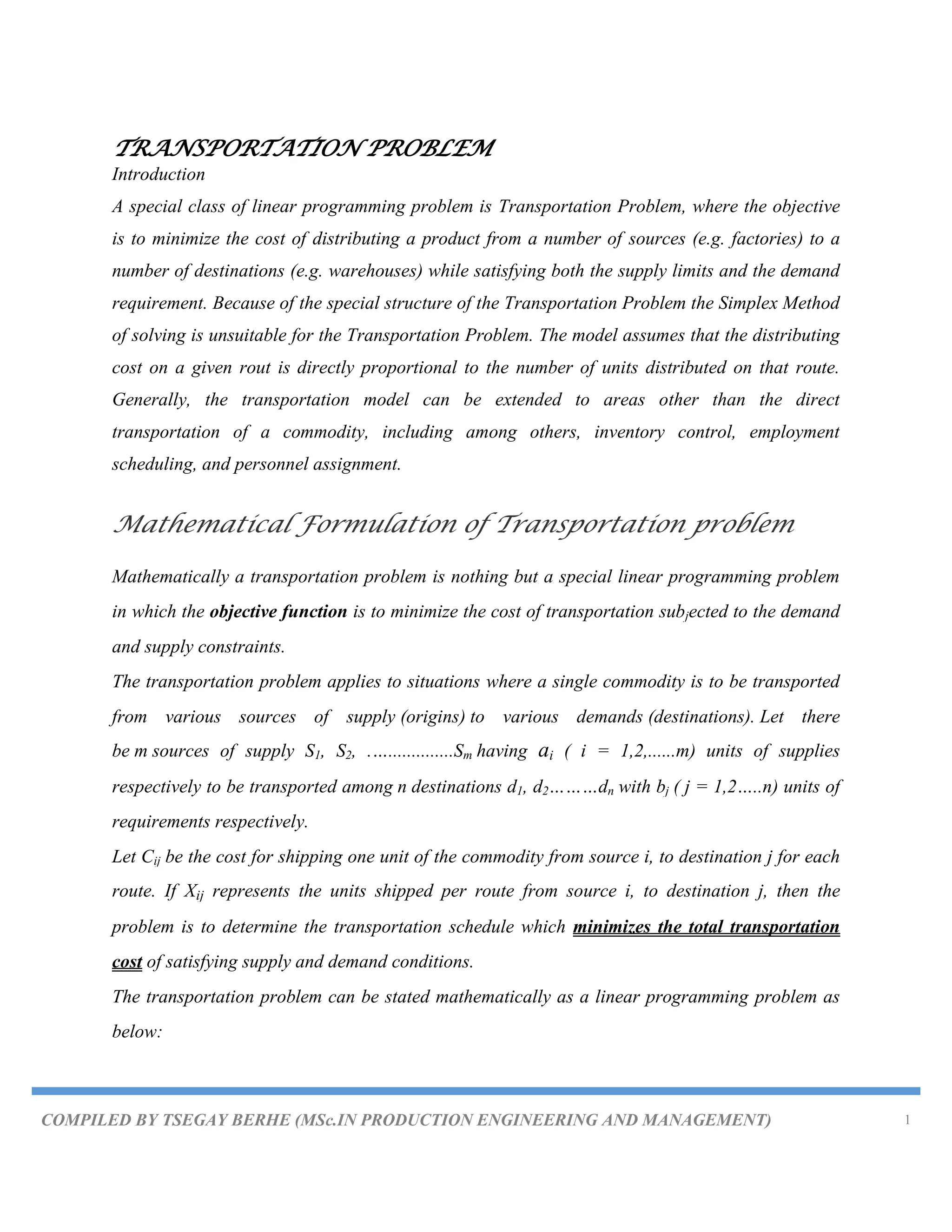
1) A mathematical formulation of transportation problems as a linear programming problem with objectives, variables, and constraints.
2) Examples of representing transportation problems using a network diagram and table.
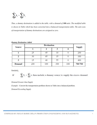
3) Methods for handling imbalanced transportation problems where supply does not equal demand, such as adding dummy rows or columns.


![COMPILED BY TSEGAY BERHE (MSc.IN PRODUCTION ENGINEERING AND MANAGEMENT) 16
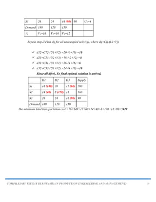
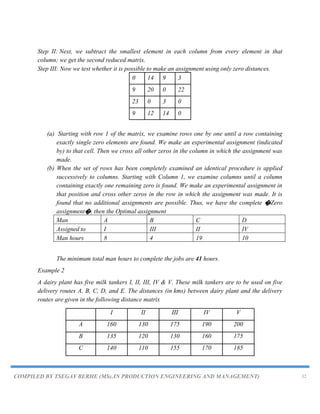
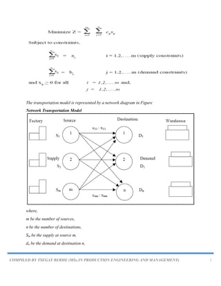
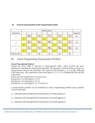
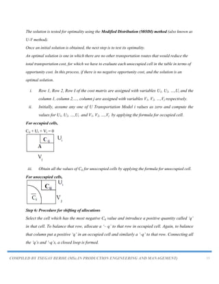
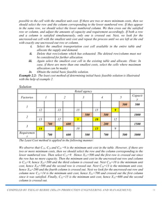
Example 2: The cost of transportation per unit from three sources[Factories] and five
destinations [Retail agency] are given in the following table Obtain the initial basic feasible
solutions using the following methods.
(i) North-west corner method
(ii) Least cost method
(iii) Vogel‟s approximation method
Retail agency
Factories 1 2 3 4 5 Capacity
1 12 13 15 15 9 500
2 13 12 9 10 12 1000
3 14 15 10 13 9 1500
Requirement 700 600 500 700 500 3000
Algorithms for all the three methods to find the initial basic feasible solution are given.
Algorithm for North-West Corner Method (NWC)
North West Corner Method:
In the northwest corner method, the largest possible allocation is made to the cell in the upper
left-hand corner of the tableau, followed by allocations to adjacent feasible cells.
The method starts at the North West (upper left) corner cell of the tableau (variable X11). With
the northwest corner method, an initial allocation is made to the cell in the upper left-hand
corner of the tableau (i.e., the “northwest corner”). The amount allocated is the most possible,
subject to the supply and demand constraints for that cell.
i. Select the North-west (i.e., upper left) corner cell of the table and allocate the
maximum possible units between the supply and demand requirements. During
allocation, the transportation cost is completely discarded (not taken into
consideration).
ii. Delete that row or column which has no values (fully exhausted) for supply or
demand.
iii. Now, with the new reduced table, again select the North-west corner cell and
allocate the available values.
iv. Repeat steps (ii) and (iii) until all the supply and demand values are zero.
v. Obtain the initial basic feasible solution.
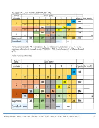
Example 2.1: Consider the problem discussed in the above Example to illustrate the North West
Corner Method of determining basic feasible solution.](https://image.slidesharecdn.com/chapter5-230820064634-de48df17/85/Chapter-5-TRANSPORTATION-PROBLEM-pdf-16-320.jpg)
![COMPILED BY TSEGAY BERHE (MSc.IN PRODUCTION ENGINEERING AND MANAGEMENT) 19
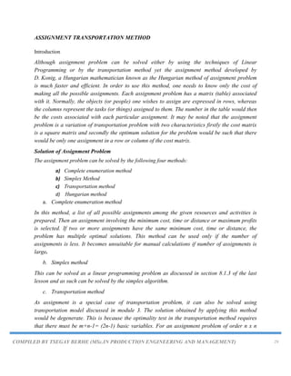
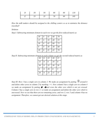
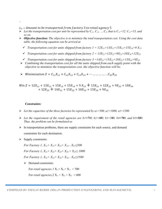
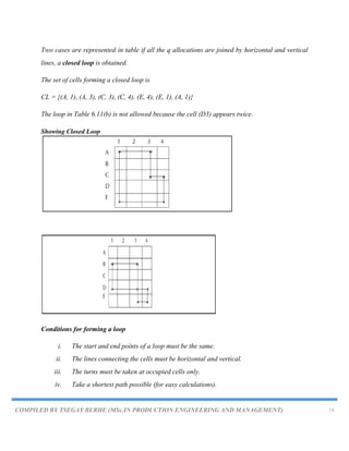
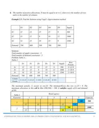
So that the basic feasible solution developed by the Least Cost Method has transportation cost is
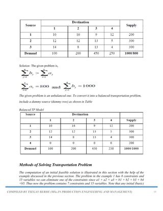
Algorithm for Vogel’s Approximation Method (VAM)
Vogel Approximation Method (VAM):
The third method for determining an initial solution, Vogel‟s approximation model (also called
VAM), is based on the concept of penalty cost or regret. If a decision maker incorrectly chooses
from several alternative courses of action, a penalty may be suffered (and the decision maker may
regret the decision that was made). In a transportation problem, the courses of action are the
alternative routes, and a wrong decision is allocating to a cell that does not contain the lowest
cost.
VAM is an improved version of the least cost method that generally produces better solutions.
The steps involved in this method are:
Step 1. For each row (column) with strictly positive capacity (requirement), determine a
penalty by subtracting the smallest unit cost element in the row (column) from the
next smallest unit cost element in the same row (column). If there are two smallest
costs, then the penalty is zero.
Step 2. Identify the row or column with the largest penalty among all the rows and
columns make allocation in the cell having the least cost in the selected row/column.
If the penalties corresponding to two or more rows or columns are equal, we select
the top most row and the extreme left column. If two or more equal penalties exist,
select one where a row/column contains minimum unit cost. If there is again a tie,
select one where maximum allocation can be made.
Step 3. We select Xij as a basic variable if Cij is the minimum cost in the row or column
with largest penalty. We choose the numerical value of Xij as high as possible subject
to the row and the column constraints. Depending upon whether ai or bj is the smaller
of the two ith row or jth column is crossed out [Delete the row/column, which has
satisfied the supply and demand.]
Step 4. The Step 2 is now performed on the uncrossed-out rows and columns until all the
basic variables have been satisfied [ Repeat steps (i) and (ii) until the entire supply
and demands are satisfied.]
Step 5. Obtain the initial basic feasible solution.
Remarks: The initial solution obtained by any of the three methods must satisfy the following
conditions:
a. The solution must be feasible, i.e., the supply and demand constraints must be satisfied (also
known as rim conditions).](https://image.slidesharecdn.com/chapter5-230820064634-de48df17/85/Chapter-5-TRANSPORTATION-PROBLEM-pdf-19-320.jpg)
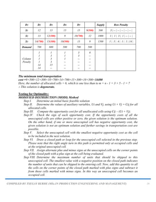
![COMPILED BY TSEGAY BERHE (MSc.IN PRODUCTION ENGINEERING AND MANAGEMENT) 25
Step IX. Repeat the whole procedure until an optimum solution is obtained.
Example
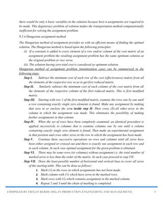
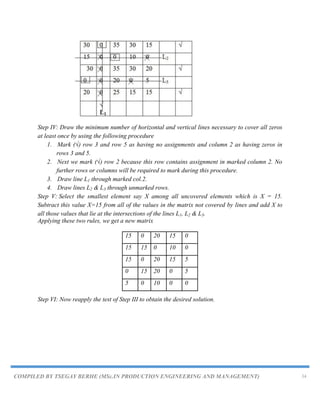
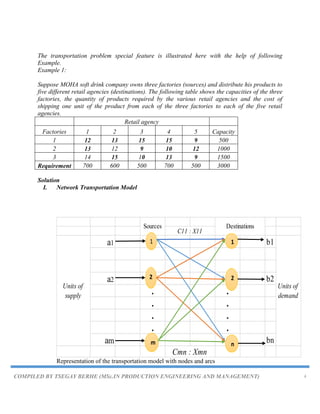
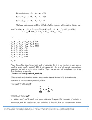
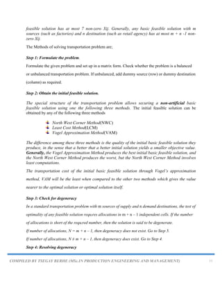
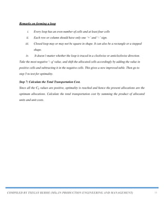
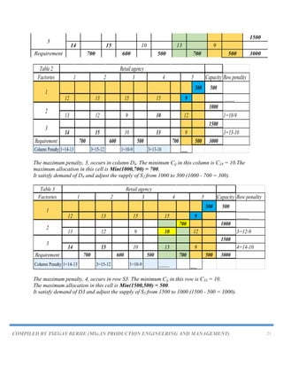
Find the optimal solution using modi method [using initial basic solution of Least Cost method].
D1 D2 D3 Supply
S1 16 20 12 200
S2 14 8 18 160
S3 26 24 16 90
Demand 180 120 150
initial basic solution by using Least Cost method
D1 D2 D3 Supply
S1 16 (50) 20 12 (150) 200
S2 14 (40) 8 (120) 18 160
S3 26 (90) 24 16 90
Demand 180 120 150
The minimum total transportation cost =16×50+12×150+14×40+8×120+26×90=6460
Here, the number of allocated cells = 5 is equal to m + n - 1 = 3 + 3 - 1 = 5
∴ This solution is non- degenerate
Optimality test using modi method...
Allocation Table is;
D1 D2 D3 Supply
S1 16 (50) 20 12 (150) 200
S2 14 (40) 8 (120) 18 160
S3 26 (90) 24 16 90
Demand 180 120 150
Iteration-1 of optimality test
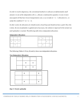
Step I.Find Ui and Vj for all occupied cells (i, j), where Cij=Ui+Vj
Let substituting, V1=0, we get](https://image.slidesharecdn.com/chapter5-230820064634-de48df17/85/Chapter-5-TRANSPORTATION-PROBLEM-pdf-25-320.jpg)
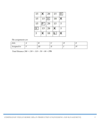
![COMPILED BY TSEGAY BERHE (MSc.IN PRODUCTION ENGINEERING AND MANAGEMENT) 26
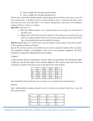
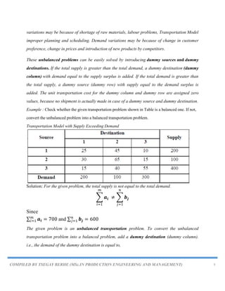
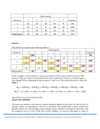
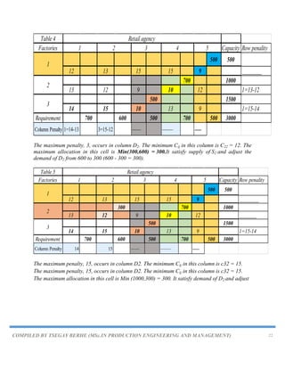
C11=U1+V1⇒U1=C11-V1⇒U1=16-0 ⇒U1=16
C13=U1+V3⇒V3=C13-U1⇒V3=12-16 ⇒V3=-4
C21=U2+V1⇒U2=C21-V1⇒U2=14-0 ⇒U2=14
C22=U2+V2⇒V2=C22-U2⇒V2=8-14 ⇒V2=-6
C31=U3+V1⇒U3=C31-V1⇒U3=26-0 ⇒U3=26
D1 D2 D3 Supply Ui
S1 16 (50) 20 12 (150) 200 U1=16
S2 14 (40) 8 (120) 18 160 U2=14
S3 26 (90) 24 16 90 U3=26
Demand 180 120 150
Vj V1=0 V2=-6 V3=-4
Step II.Find dij for all unoccupied cells (i, j), where dij=Cij-(Ui+Vj)
d12=C12-(U1+V2) =20-(16-6) =10
d23=C23-(U2+V3) =18-(14-4) =8
d32=C32-(U3+V2) =24-(26-6) =4
d33=C33-(U3+V3) =16-(26-4) =-6
D1 D2 D3 Supply ui
S1 16 (50) 20 [10] 12 (150) 200 U1=16
S2 14 (40) 8 (120) 18 [8] 160 U2=14
S3 26 (90) 24 [4] 16 [-6] 90 U3=26
Demand 180 120 150
Vj V1=0 V2=-6 V3=-4
Step III. Now choose the minimum negative value from all dij (opportunity cost) = d33 = [-6]
and draw a closed path from S3D3
Now choose the minimum negative value from all dij (opportunity cost) = d33 = [-6] and draw
a closed path from S3D3.
Closed path is S3D3→S3D1→S1D1→S1D3
Closed path and plus/minus sign allocation.](https://image.slidesharecdn.com/chapter5-230820064634-de48df17/85/Chapter-5-TRANSPORTATION-PROBLEM-pdf-26-320.jpg)
![COMPILED BY TSEGAY BERHE (MSc.IN PRODUCTION ENGINEERING AND MANAGEMENT) 27
D1 D2 D3 Supply Ui
S1 16 (50)
(+)
20 [10] 12 (150)
(-)
200 U1=16
S2 14 (40) 8 (120) 18 [8] 160 U2=14
S3 26 (90)
(-)
24 [4] 16 [-6]
(+)
90 U3=26
Demand 180 120 150
Vj V1=0 V2=-6 V3=-4
Step IV.Minimum allocated value among all negative position (-) on closed path = 90.
Substract 90 from all (-) and Add it to all (+)
D1 D2 D3 Supply
S1 16 (140) 20 12 (60) 200
S2 14 (40) 8 (120) 18 160
S3 26 24 16 (90) 90
Demand 180 120 150
Step V.Repeat the step 1 to 4, until an optimal solution is obtained
Iteration-2 of optimality test
Find Ui and Vj for all occupied cells(i,j), where Cij=Ui+Vj
Let substituting, U1=0, we get
C11=U1+V1⇒V1=C11-U1⇒V1=16-0 ⇒V1=16
C21=U2+V1⇒U2=C21-V1⇒U2=14-16 ⇒U2=-2
C22=U2+V2⇒V2=C22-U2⇒V2=8+2 ⇒V2=10
C13=U1+V3⇒V3=C13-U1⇒V3=12-0 ⇒V3=12
C33=U3+V3⇒U3=C33-V3⇒U3=16-12 ⇒U3=4
D1 D2 D3 Supply Ui
S1 16 (140) 20 12 (60) 200 U1=0
S2 14 (40) 8 (120) 18 160 U2=-2](https://image.slidesharecdn.com/chapter5-230820064634-de48df17/85/Chapter-5-TRANSPORTATION-PROBLEM-pdf-27-320.jpg)