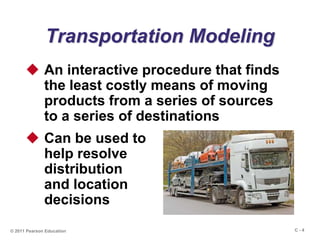
Submit Search
Upload
transportation_model (4).ppt
•
Download as PPT, PDF
•
0 likes
•
9 views
A
ArepuriDeepthi
Follow
operations and management
Read less
Read more
Science
Report
Share
Report
Share
1 of 44
Download now
Recommended
Heizer om10 mod_c
Heizer om10 mod_c
ryaekle
Transportation model powerpoint
Giselle Gaas
qtm
Chap 10
Chap 10
geet232
Quantitative Analysis for Management, 11e (Render)
Transportation problems1
Firas Husseini
This presentation is made to represent the basic transportation model. The aim of this presentation is to implement the transportation model in solving transportation problem.
Transportation model
msn007
Transportation Problem
Transportation problem
Abhimanyu Verma
Transportation Problems
5. transportation problems
Hakeem-Ur- Rehman
pom 10th ed ch8
Productions & Operations Management Chapter 08
jncgw5t6xq
for aiub summar , for semister break preparation
9. transportation model
Sudipta Saha
Quantitative Analysis for Management, 11e (Render)
Rsh qam11 ch09 ge
Rsh qam11 ch09 ge
Firas Husseini
Deepika(14 mba5012) transportation ppt
Deepika Bansal
presentation for my Quanti class...
Pa 906.transportation problem and algorithms final
hsur2010
Transportation Modelling - Quantitative Analysis and Discrete Maths
Krupesh Shah
Transportation models
Robejhon de Villena
Assign transportation
Kinshook Chaturvedi
m2
Ms(transp.transship,assign) (1)
kongara
chapter three lecture note on psychometrics course
CHAPTER THREE QABD 2016.pptx
DejeneDay
The transportation problem is a special type of linear programming problem where the objective is to minimize the cost of distributing a product from a number of sources or origins to a number of destinations. Because of its special structure, the usual simplex method is not suitable for solving transportation problems. These problems require a special method of solution.
Transportation problems
VishalHotchandani2
Notes
O.R UNIT 3.pdf
O.R UNIT 3.pdf
SaifAliKhan898691
Transportation Model described
transportation-model.ppt
anubhuti18
operation reserch
Transportation model and assignment model
priyanka yadav
Quantitative
QA CHAPTER III and IV(1)(1).pdf
Teshome48
Transportationproblem 111218100045-phpapp01
RAJUMARU3
operations research chapter three
chapter 3.pptx
chapter 3.pptx
DejeneDay
Northwest Corner Rule - Phase 1 Stepping Stone Method - Phase 2
Transportation Problem
Alvin Niere
Vogel's Approximation Method & Modified Distribution Method
Kaushik Maitra
Transportation, Assignment, Transshipment, Hungarian models
Bba 3274 qm week 9 transportation and assignment models
Stephen Ong
Transportation
Transportation.pptx
Transportation.pptx
SauravDash10
The return of a sample of near-surface atmosphere from Mars would facilitate answers to several first-order science questions surrounding the formation and evolution of the planet. One of the important aspects of terrestrial planet formation in general is the role that primary atmospheres played in influencing the chemistry and structure of the planets and their antecedents. Studies of the martian atmosphere can be used to investigate the role of a primary atmosphere in its history. Atmosphere samples would also inform our understanding of the near-surface chemistry of the planet, and ultimately the prospects for life. High-precision isotopic analyses of constituent gases are needed to address these questions, requiring that the analyses are made on returned samples rather than in situ.
THE IMPORTANCE OF MARTIAN ATMOSPHERE SAMPLE RETURN.
Sérgio Sacani
Hadean zircons provide a potential record of Earth's earliest subduction 4.3 billion years ago. Itremains enigmatic how subduction could be initiated so soon after the presumably Moon‐forming giant impact(MGI). Earlier studies found an increase in Earth's core‐mantle boundary (CMB) temperature due to theaccumulation of the impactor's core, and our recent work shows Earth's lower mantle remains largely solid, withsome of the impactor's mantle potentially surviving as the large low‐shear velocity provinces (LLSVPs). Here,we show that a hot post‐impact CMB drives the initiation of strong mantle plumes that can induce subductioninitiation ∼200 Myr after the MGI. 2D and 3D thermomechanical computations show that a high CMBtemperature is the primary factor triggering early subduction, with enrichment of heat‐producing elements inLLSVPs as another potential factor. The models link the earliest subduction to the MGI with implications forunderstanding the diverse tectonic regimes of rocky planets.
A Giant Impact Origin for the First Subduction on Earth
Sérgio Sacani
More Related Content
Similar to transportation_model (4).ppt
for aiub summar , for semister break preparation
9. transportation model
Sudipta Saha
Quantitative Analysis for Management, 11e (Render)
Rsh qam11 ch09 ge
Rsh qam11 ch09 ge
Firas Husseini
Deepika(14 mba5012) transportation ppt
Deepika Bansal
presentation for my Quanti class...
Pa 906.transportation problem and algorithms final
hsur2010
Transportation Modelling - Quantitative Analysis and Discrete Maths
Krupesh Shah
Transportation models
Robejhon de Villena
Assign transportation
Kinshook Chaturvedi
m2
Ms(transp.transship,assign) (1)
kongara
chapter three lecture note on psychometrics course
CHAPTER THREE QABD 2016.pptx
DejeneDay
The transportation problem is a special type of linear programming problem where the objective is to minimize the cost of distributing a product from a number of sources or origins to a number of destinations. Because of its special structure, the usual simplex method is not suitable for solving transportation problems. These problems require a special method of solution.
Transportation problems
VishalHotchandani2
Notes
O.R UNIT 3.pdf
O.R UNIT 3.pdf
SaifAliKhan898691
Transportation Model described
transportation-model.ppt
anubhuti18
operation reserch
Transportation model and assignment model
priyanka yadav
Quantitative
QA CHAPTER III and IV(1)(1).pdf
Teshome48
Transportationproblem 111218100045-phpapp01
RAJUMARU3
operations research chapter three
chapter 3.pptx
chapter 3.pptx
DejeneDay
Northwest Corner Rule - Phase 1 Stepping Stone Method - Phase 2
Transportation Problem
Alvin Niere
Vogel's Approximation Method & Modified Distribution Method
Kaushik Maitra
Transportation, Assignment, Transshipment, Hungarian models
Bba 3274 qm week 9 transportation and assignment models
Stephen Ong
Transportation
Transportation.pptx
Transportation.pptx
SauravDash10
Similar to transportation_model (4).ppt
(20)
9. transportation model
Rsh qam11 ch09 ge
Rsh qam11 ch09 ge
Deepika(14 mba5012) transportation ppt
Pa 906.transportation problem and algorithms final
Transportation Modelling - Quantitative Analysis and Discrete Maths
Transportation models
Assign transportation
Ms(transp.transship,assign) (1)
CHAPTER THREE QABD 2016.pptx
Transportation problems
O.R UNIT 3.pdf
O.R UNIT 3.pdf
transportation-model.ppt
Transportation model and assignment model
QA CHAPTER III and IV(1)(1).pdf
Transportationproblem 111218100045-phpapp01
chapter 3.pptx
chapter 3.pptx
Transportation Problem
Vogel's Approximation Method & Modified Distribution Method
Bba 3274 qm week 9 transportation and assignment models
Transportation.pptx
Transportation.pptx
Recently uploaded
The return of a sample of near-surface atmosphere from Mars would facilitate answers to several first-order science questions surrounding the formation and evolution of the planet. One of the important aspects of terrestrial planet formation in general is the role that primary atmospheres played in influencing the chemistry and structure of the planets and their antecedents. Studies of the martian atmosphere can be used to investigate the role of a primary atmosphere in its history. Atmosphere samples would also inform our understanding of the near-surface chemistry of the planet, and ultimately the prospects for life. High-precision isotopic analyses of constituent gases are needed to address these questions, requiring that the analyses are made on returned samples rather than in situ.
THE IMPORTANCE OF MARTIAN ATMOSPHERE SAMPLE RETURN.
Sérgio Sacani
Hadean zircons provide a potential record of Earth's earliest subduction 4.3 billion years ago. Itremains enigmatic how subduction could be initiated so soon after the presumably Moon‐forming giant impact(MGI). Earlier studies found an increase in Earth's core‐mantle boundary (CMB) temperature due to theaccumulation of the impactor's core, and our recent work shows Earth's lower mantle remains largely solid, withsome of the impactor's mantle potentially surviving as the large low‐shear velocity provinces (LLSVPs). Here,we show that a hot post‐impact CMB drives the initiation of strong mantle plumes that can induce subductioninitiation ∼200 Myr after the MGI. 2D and 3D thermomechanical computations show that a high CMBtemperature is the primary factor triggering early subduction, with enrichment of heat‐producing elements inLLSVPs as another potential factor. The models link the earliest subduction to the MGI with implications forunderstanding the diverse tectonic regimes of rocky planets.
A Giant Impact Origin for the First Subduction on Earth
Sérgio Sacani
NuGOweek 2024 programme
NuGOweek 2024 Ghent - programme - final version
pablovgd
Pineal gland
Mammalian Pineal Body Structure and Also Functions
YOGESH DOGRA
Mammals have dominated Earth for approximately 55 Myr thanks to their adaptations and resilience to warming and cooling during the Cenozoic. All life will eventually perish in a runaway greenhouse once absorbed solar radiation exceeds the emission of thermal radiation in several billions of years. However, conditions rendering the Earth naturally inhospitable to mammals may develop sooner because of long-term processes linked to plate tectonics (short-term perturbations are not considered here). In ~250 Myr, all continents will converge to form Earth’s next supercontinent, Pangea Ultima. A natural consequence of the creation and decay of Pangea Ultima will be extremes in pCO2 due to changes in volcanic rifting and outgassing. Here we show that increased pCO2, solar energy (F⨀; approximately +2.5% W m−2 greater than today) and continentality (larger range in temperatures away from the ocean) lead to increasing warming hostile to mammalian life. We assess their impact on mammalian physiological limits (dry bulb, wet bulb and Humidex heat stress indicators) as well as a planetary habitability index. Given mammals’ continued survival, predicted background pCO2 levels of 410–816 ppm combined with increased F⨀ will probably lead to a climate tipping point and their mass extinction. The results also highlight how global landmass configuration, pCO2 and F⨀ play a critical role in planetary habitability.
Climate extremes likely to drive land mammal extinction during next supercont...
Sérgio Sacani
Biotech M pharma 2nd send' dr harisingh gour sagar university
biotech-regenration of plants, pharmaceutical applications.pptx
ANONYMOUS
Normal Cell Metabolism: Cellular respiration describes the series of steps that cells use to break down sugar and other chemicals to get the energy we need to function. Energy is stored in the bonds of glucose and when glucose is broken down, much of that energy is released. Cell utilize energy in the form of ATP. The first step of respiration is called glycolysis. In a series of steps, glycolysis breaks glucose into two smaller molecules - a chemical called pyruvate. A small amount of ATP is formed during this process. Most healthy cells continue the breakdown in a second process, called the Kreb's cycle. The Kreb's cycle allows cells to “burn” the pyruvates made in glycolysis to get more ATP. The last step in the breakdown of glucose is called oxidative phosphorylation (Ox-Phos). It takes place in specialized cell structures called mitochondria. This process produces a large amount of ATP. Importantly, cells need oxygen to complete oxidative phosphorylation. If a cell completes only glycolysis, only 2 molecules of ATP are made per glucose. However, if the cell completes the entire respiration process (glycolysis - Kreb's - oxidative phosphorylation), about 36 molecules of ATP are created, giving it much more energy to use. IN CANCER CELL: Unlike healthy cells that "burn" the entire molecule of sugar to capture a large amount of energy as ATP, cancer cells are wasteful. Cancer cells only partially break down sugar molecules. They overuse the first step of respiration, glycolysis. They frequently do not complete the second step, oxidative phosphorylation. This results in only 2 molecules of ATP per each glucose molecule instead of the 36 or so ATPs healthy cells gain. As a result, cancer cells need to use a lot more sugar molecules to get enough energy to survive. Unlike healthy cells that "burn" the entire molecule of sugar to capture a large amount of energy as ATP, cancer cells are wasteful. Cancer cells only partially break down sugar molecules. They overuse the first step of respiration, glycolysis. They frequently do not complete the second step, oxidative phosphorylation. This results in only 2 molecules of ATP per each glucose molecule instead of the 36 or so ATPs healthy cells gain. As a result, cancer cells need to use a lot more sugar molecules to get enough energy to survive. introduction to WARBERG PHENOMENA: WARBURG EFFECT Usually, cancer cells are highly glycolytic (glucose addiction) and take up more glucose than do normal cells from outside. Otto Heinrich Warburg (; 8 October 1883 – 1 August 1970) In 1931 was awarded the Nobel Prize in Physiology for his "discovery of the nature and mode of action of the respiratory enzyme. WARNBURG EFFECT : cancer cells under aerobic (well-oxygenated) conditions to metabolize glucose to lactate (aerobic glycolysis) is known as the Warburg effect. Warburg made the observation that tumor slices consume glucose and secrete lactate at a higher rate than normal tissues.
Cancer cell metabolism: special Reference to Lactate Pathway
AADYARAJPANDEY1
Analytical chemistry
SAMPLING.pptx for analystical chemistry sample techniques
rodneykiptoo8
Article written for leader telegram
Astronomy Update- Curiosity’s exploration of Mars _ Local Briefs _ leadertele...
NathanBaughman3
Liquid viscosity lab report
Lab report on liquid viscosity of glycerin
ossaicprecious19
PESTS OF SUGARCANE - BORERS BORERS 1. Early shoot borer, Chilo infuscatellus, Crambidae, Lepidoptera Symptom of damage: Deadheart in 1-3 month old crop, which can be easily pulled out, rotten portion of the straw coloured dead-heart emits an offensive odour. A number of bore holes at the base of the shoot just above the ground level. Nature of damage: Caterpillar bores into the central shoot and feeds on the internal tissue. This cause interference in the translocation of plant sap and damage the sugar storing tissues. Egg: Flat-scale like eggs are laid in 3-5 rows on the lower surface of leaves in masses of 4-100. The masses are slightly overlapping like tiles. Larva: Larva is dirty white with five dark violet longitudinal stripes and dark brown head. Pupa: Pupation takes place within the tunnel. Caterpillar before pupating makes a large exit hole in the stem and blocks the opening with silken discs. Adult: Pale greyish brown moth with black dots near the costal margin of the forewings and with white hindwings. 2. Internode borer, Chilo sacchariphagus indicus, Crambidae, Lepidoptera Symptom of damage: Internodes constricted and shortened, with a number of boreholes and fresh excreta in the nodal region. Affected tissues reddened. Nature of damage: Caterpillars attack sugarcane plants after 3 months of planting. They bore into the canes near the nodes; entry holes are plugged with excreta. Entry is generally confined to the first five internodes. Egg: Scale-like white eggs are laid by female moths in batches of 9-11, near the midribs, on leaf sheaths or on stem. Larva: White larva with four violet longitudinal stripes and light brown head. Pupa: Pupation takes place in semi-dried leaf sheath. Adult: Pale brown with white hind wings. 3. Top borer, Scirpophaga excerptalis, Pyralidae, Lepidoptera Symptom of damage: Deadheart in grownup canes, which cannot be easily pulled; deadheart reddish brown in colour; parallel row of shot holes in the emerging leaves and red tunnels in the midribs of leaves; bunchy tip due to the growth of side shoots. Nature of damage: Caterpillars are mainly found in the apical portion of the canes, boring through the growing point and down the upper joints until it reaches the sappy portion of the stem, there it feeds on the tissues and destroys the cane. They also bore into the unfolded leaves preferably into the midrib, mining its way to the base. Egg: Eggs are laid on the lower surface of top leaves in clusters particularly near midribs. The clusters are covered with buff coloured hairs. Larva :Smooth, white or cream coloured with a red coloured mid-dorsal line and yellow head. Pupa: Pupation takes place within the larval tunnel in a chamber with an exit hole constructed by the caterpillar. Adult: White coloured moth (with a buff coloured anal tuft in the abdominal tip of female).
Pests of sugarcane_Binomics_IPM_Dr.UPR.pdf
PirithiRaju
double halide perovskite
Shuaib Y-basedComprehensive mahmudj.pptx
MdAbuRayhan16
Since the loophole-free Bell experiments of 2020 and the Nobel prizes in physics of 2022, critics of Bell's work have retreated to the fortress of super-determinism. Now, super-determinism is a derogatory word - it just means "determinism". Palmer, Hance and Hossenfelder argue that quantum mechanics and determinism are not incompatible, using a sophisticated mathematical construction based on a subtle thinning of allowed states and measurements in quantum mechanics, such that what is left appears to make Bell's argument fail, without altering the empirical predictions of quantum mechanics. I think however that it is a smoke screen, and the slogan "lost in math" comes to my mind. I will discuss some other recent disproofs of Bell's theorem using the language of causality based on causal graphs. Causal thinking is also central to law and justice. I will mention surprising connections to my work on serial killer nurse cases, in particular the Dutch case of Lucia de Berk and the current UK case of Lucy Letby.
Richard's entangled aventures in wonderland
Richard Gill
The ASGCT Annual Meeting was packed with exciting progress in the field advancing efforts to deliver highly promising therapies to more patients.
The ASGCT Annual Meeting was packed with exciting progress in the field advan...
Health Advances
electrochemical gass sensors
electrochemical gas sensors and their uses.pptx
Husna Zaheer
PLATELETS
platelets- lifespan -Clot retraction-disorders.pptx
muralinath2
Microbial Type Culture Collection (MTCC)
abhishekdhamu51
Nutrition is the science that deals with the study of nutrients and their role in maintaining human health and well-being. It encompasses the various processes involved in the intake, absorption, and utilization of essential nutrients, such as carbohydrates, proteins, fats, vitamins, minerals, and water, by the human body.
GLOBAL AND LOCAL SCENARIO OF FOOD AND NUTRITION.pptx
SultanMuhammadGhauri
The ambient solar wind that flls the heliosphere originates from multiple sources in the solar corona and is highly structured. It is often described as high-speed, relatively homogeneous, plasma streams from coronal holes and slow-speed, highly variable, streams whose source regions are under debate. A key goal of ESA/NASA’s Solar Orbiter mission is to identify solar wind sources and understand what drives the complexity seen in the heliosphere. By combining magnetic feld modelling and spectroscopic techniques with high-resolution observations and measurements, we show that the solar wind variability detected in situ by Solar Orbiter in March 2022 is driven by spatio-temporal changes in the magnetic connectivity to multiple sources in the solar atmosphere. The magnetic feld footpoints connected to the spacecraft moved from the boundaries of a coronal hole to one active region (12961) and then across to another region (12957). This is refected in the in situ measurements, which show the transition from fast to highly Alfvénic then to slow solar wind that is disrupted by the arrival of a coronal mass ejection. Our results describe solar wind variability at 0.5 au but are applicable to near-Earth observatories.
Multi-source connectivity as the driver of solar wind variability in the heli...
Sérgio Sacani
documents provide information about insect classification and taxonomy of insect
insect taxonomy importance systematics and classification
anitaento25
Recently uploaded
(20)
THE IMPORTANCE OF MARTIAN ATMOSPHERE SAMPLE RETURN.
A Giant Impact Origin for the First Subduction on Earth
NuGOweek 2024 Ghent - programme - final version
Mammalian Pineal Body Structure and Also Functions
Climate extremes likely to drive land mammal extinction during next supercont...
biotech-regenration of plants, pharmaceutical applications.pptx
Cancer cell metabolism: special Reference to Lactate Pathway
SAMPLING.pptx for analystical chemistry sample techniques
Astronomy Update- Curiosity’s exploration of Mars _ Local Briefs _ leadertele...
Lab report on liquid viscosity of glycerin
Pests of sugarcane_Binomics_IPM_Dr.UPR.pdf
Shuaib Y-basedComprehensive mahmudj.pptx
Richard's entangled aventures in wonderland
The ASGCT Annual Meeting was packed with exciting progress in the field advan...
electrochemical gas sensors and their uses.pptx
platelets- lifespan -Clot retraction-disorders.pptx
Microbial Type Culture Collection (MTCC)
GLOBAL AND LOCAL SCENARIO OF FOOD AND NUTRITION.pptx
Multi-source connectivity as the driver of solar wind variability in the heli...
insect taxonomy importance systematics and classification
transportation_model (4).ppt
1.
C - 1 ©
2011 Pearson Education C Transportation Modeling PowerPoint presentation to accompany Heizer and Render Operations Management, 10e, Global Edition Principles of Operations Management, 8e, Global Edition PowerPoint slides by Jeff Heyl
2.
C - 2 ©
2011 Pearson Education Outline Transportation Modeling Developing an Initial Solution The Northwest-Corner Rule The Intuitive Lowest-Cost Method The Stepping-Stone Method Special Issues in Modeling Demand Not Equal to Supply Degeneracy
3.
C - 3 ©
2011 Pearson Education Learning Objectives When you complete this module you should be able to: 1. Develop an initial solution to a transportation models with the northwest-corner and intuitive lowest-cost methods 2. Solve a problem with the stepping- stone method 3. Balance a transportation problem 4. Solve a problem with degeneracy
4.
C - 4 ©
2011 Pearson Education Transportation Modeling An interactive procedure that finds the least costly means of moving products from a series of sources to a series of destinations Can be used to help resolve distribution and location decisions
5.
C - 5 ©
2011 Pearson Education Transportation Modeling A special class of linear programming Need to know 1. The origin points and the capacity or supply per period at each 2. The destination points and the demand per period at each 3. The cost of shipping one unit from each origin to each destination
6.
C - 6 Transportation
example • The following example was used to demonstrate the formulation of the transportation model. • Bath tubes are produced in plants in three different cities—Des Moines , Evansville , and Fort Lauder , tube is shipped to the distributers in railroad , . Each plant is able to supply the following number of units , Des Moines 100 units, Evansville 300 units and Fort Lauder 300 units • tubes will shipped to the distributers in three cities Albuquerque , Boston, and Cleveland ,the distribution requires the following unites ; Albuquerque 300 units , Boston 200 units and Cleveland 200 units © 2011 Pearson Education
7.
C - 7 ©
2011 Pearson Education Shipping cost per unit To From Albuquerque Boston Cleveland Des Moines $5 $4 $3 Evansville $8 $4 $3 Fort Lauder $9 $7 $5 Table C.1
8.
C - 8 ©
2011 Pearson Education Transportation Problem Fort Lauder (300 units capacity) Albuquerque (300 units required) Des Moines (100 units capacity) Evansville (300 units capacity) Cleveland (200 units required) Boston (200 units required) Figure C.1
9.
C - 9 ©
2011 Pearson Education Transportation Matrix From To Albuquerque Boston Cleveland Des Moines Evansville Fort Lauder Factory capacity Warehouse requirement 300 300 300 200 200 100 700 $5 $5 $4 $4 $3 $3 $9 $8 $7 Cost of shipping 1 unit from Fort Lauder factory to Boston warehouse Des Moines capacity constraint Cell representing a possible source-to- destination shipping assignment (Evansville to Cleveland) Total demand and total supply Cleveland warehouse demand Figure C.2
10.
C - 10 ©
2011 Pearson Education • Check the equality of the total supply & demand (if not, then we need for dummy solution ) • how many ship of unit should be transported from each demand to each distribution center can be expressed as (Xij) • i ……..for demand and j …….for distribution center
11.
C - 11 Step
2 Establish the initial feasible solution The Northwest corner rule Least Cost Method Vogel’s Approximation Model © 2011 Pearson Education
12.
C - 12 ©
2011 Pearson Education Northwest-Corner Rule Start in the upper left-hand cell (or northwest corner) of the table and allocate units to shipping routes as follows: 1. Exhaust the supply (factory capacity) of each row before moving down to the next row 2. Exhaust the (warehouse) requirements of each column before moving to the next column 3. Check to ensure that all supplies and demands are met
13.
C - 13 •
The steps of the northwest corner method are summarized here: • 1. Allocate as much as possible to the cell in the upper left-hand corner, subject to the supply and demand constraints. • 2. Allocate as much as possible to the next adjacent feasible cell. • 3. Repeat step 1,2 until all units all supply and demand have been satisfied © 2011 Pearson Education
14.
C - 14 ©
2011 Pearson Education Northwest-Corner Rule 1. Assign 100 tubs from Des Moines to Albuquerque (exhausting Des Moines’s supply) 2. Assign 200 tubs from Evansville to Albuquerque (exhausting Albuquerque’s demand) 3. Assign 100 tubs from Evansville to Boston (exhausting Evansville’s supply) 4. Assign 100 tubs from Fort Lauder to Boston (exhausting Boston’s demand) 5. Assign 200 tubs from Fort Lauderdale to Cleveland (exhausting Cleveland’s demand and Fort Lauder’s supply)
15.
C - 15 ©
2011 Pearson Education To (A) Albuquerque (B) Boston (C) Cleveland (D) Des Moines (E) Evansville (F) Fort Lauder Warehouse requirement 300 200 200 Factory capacity 300 300 100 700 $5 $5 $4 $4 $3 $3 $9 $8 $7 From Northwest-Corner Rule 100 100 100 200 200 Figure C.3 Means that the firm is shipping 100 bathtubs from Fort Lauder to Boston
16.
C - 16 ©
2011 Pearson Education Northwest-Corner Rule Computed Shipping Cost Table C.2 This is a feasible solution but not necessarily the lowest cost alternative (not the optimal solution) Route From To Tubs Shipped Cost per Unit Total Cost D A 100 $5 $ 500 E A 200 8 1,600 E B 100 4 400 F B 100 7 700 F C 200 5 $1,000 Total: $4,200
17.
C - 17 ©
2011 Pearson Education Second Method The Lowest-Cost Method 1. Evaluate the transportation cost and select the square with the lowest cost (in case a Tie make an arbitrary selection ). 2. Depending upon the supply & demand condition , allocate the maximum possible units to lowest cost square. 3. Delete the satisfied allocated row or the column (or both). 4. Repeat steps 1 and 3 until all units have been allocated.
18.
C - 18 ©
2011 Pearson Education The Lowest-Cost Method To (A) Albuquerque (B) Boston (C) Cleveland (D) Des Moines (E) Evansville (F) Fort Lauder Warehouse requirement 300 200 200 Factory capacity 300 300 100 700 $5 $5 $4 $4 $3 $3 $9 $8 $7 From 100 First, $3 is the lowest cost cell so ship 100 units from Des Moines to Cleveland and cross off the first row as Des Moines is satisfied Figure C.4
19.
C - 19 ©
2011 Pearson Education The Lowest-Cost Method To (A) Albuquerque (B) Boston (C) Cleveland (D) Des Moines (E) Evansville (F) Fort Lauderdale Warehouse requirement 300 200 200 Factory capacity 300 300 100 700 $5 $5 $4 $4 $3 $3 $9 $8 $7 From 100 100 Second, $3 is again the lowest cost cell so ship 100 units from Evansville to Cleveland and cross off column C as Cleveland is satisfied Figure C.4
20.
C - 20 ©
2011 Pearson Education The Lowest-Cost Method To (A) Albuquerque (B) Boston (C) Cleveland (D) Des Moines (E) Evansville (F) Fort Lauderdale Warehouse requirement 300 200 200 Factory capacity 300 300 100 700 $5 $5 $4 $4 $3 $3 $9 $8 $7 From 100 100 200 Third, $4 is the lowest cost cell so ship 200 units from Evansville to Boston and cross off column B and row E as Evansville and Boston are satisfied Figure C.4
21.
C - 21 ©
2011 Pearson Education The Lowest-Cost Method To (A) Albuquerque (B) Boston (C) Cleveland (D) Des Moines (E) Evansville (F) Fort Lauderdale Warehouse requirement 300 200 200 Factory capacity 300 300 100 700 $5 $5 $4 $4 $3 $3 $9 $8 $7 From 100 100 200 300 Finally, ship 300 units from Albuquerque to Fort Lauder as this is the only remaining cell to complete the allocations Figure C.4
22.
C - 22 ©
2011 Pearson Education The Lowest-Cost Method To (A) Albuquerque (B) Boston (C) Cleveland (D) Des Moines (E) Evansville (F) Fort Lauderdale Warehouse requirement 300 200 200 Factory capacity 300 300 100 700 $5 $5 $4 $4 $3 $3 $9 $8 $7 From 100 100 200 300 Total Cost = $3(100) + $3(100) + $4(200) + $9(300) = $4,100 Figure C.4
23.
C - 23 ©
2011 Pearson Education The Lowest-Cost Method To (A) Albuquerque (B) Boston (C) Cleveland (D) Des Moines (E) Evansville (F) Fort Lauderdale Warehouse requirement 300 200 200 Factory capacity 300 300 100 700 $5 $5 $4 $4 $3 $3 $9 $8 $7 From 100 100 200 300 Total Cost = $3(100) + $3(100) + $4(200) + $9(300) = $4,100 Figure C.4 This is a feasible solution, and an improvement over the previous solution, but not necessarily the lowest cost alternative
24.
C - 24 ©
2011 Pearson Education The Lowest-Cost Method Computed Shipping Cost Table C.2 This is a feasible solution but not necessarily the lowest cost alternative (not the optimal solution) Route From To Tubs Shipped Cost per Unit Total Cost D C 100 $3 $ 300 E C 200 3 600 E B 200 4 800 F A 300 9 2700 Total: $4,100
25.
C - 25 Testing
the initial feasible solution • Test for optimality • Optimal solution is achieved when there is no other alternative solution give lower cost. • Two method for the optimal solution :- • Stepping stone method • Modified Distribution method (MODM) © 2011 Pearson Education
26.
C - 26 ©
2011 Pearson Education Stepping-Stone Method 1. Proceed row by row and Select a water square (a square without any allocation) to evaluate 2. Beginning at this square, trace/forming a closed path back to the original square via squares that are currently being used. 3. Beginning with a plus (+) sign at the unused corner (water square), place alternate minus and plus signs at each corner of the path just traced.
27.
C - 27 ©
2011 Pearson Education 4. Calculate an improvement index (the net cost change for the path )by first adding the unit-cost figures found in each square containing a plus sign and subtracting the unit costs in each square containing a minus sign. 5. Repeat steps 1 though 4 until you have calculated an improvement index for all unused squares.
28.
C - 28 •
Evaluate the solution from optimality test by observing the sign of the net cost change I. The negative sign (-) indicates that a cost reduction can be made by making the change. II. Zero result indicates that there will be no change in cost. III. The positive sign (+) indicates an increase in cost if the change is made. IV.If all the signs are positive , it means that the optimal solution has been reached . V. If more than one squares have a negative signs then the water squared with the largest negative net cost change is selected for quicker solution , in case of tie; choose one of them randomly. © 2011 Pearson Education
29.
C - 29 ©
2011 Pearson Education 6. If an improvement is possible, choose the route (unused square) with the largest negative improvement index 7. On the closed path for that route, select the smallest number found in the squares containing minus signs, adding this number to all squares on the closed path with plus signs and subtract it from all squares with a minus sign .Repeat these process until you have evaluate all unused squares 8. Prepare the new transportation table and check for the optimality.
30.
C - 30 ©
2011 Pearson Education $5 $8 $4 $4 + - + - Stepping-Stone Method To (A) Albuquerque (B) Boston (C) Cleveland (D) Des Moines (E) Evansville (F) Fort Lauderdale Warehouse requirement 300 200 200 Factory capacity 300 300 100 700 $5 $5 $4 $4 $3 $3 $9 $8 $7 From 100 100 100 200 200 + - - + 1 100 201 99 99 100 200 Figure C.5 Des Moines- Boston index = $4 - $5 + $8 - $4 = +$3
31.
C - 31 ©
2011 Pearson Education Stepping-Stone Method To (A) Albuquerque (B) Boston (C) Cleveland (D) Des Moines (E) Evansville (F) Fort Lauder Warehouse requirement 300 200 200 Factory capacity 300 300 100 700 $5 $5 $4 $4 $3 $3 $9 $8 $7 From 100 100 100 200 200 Figure C.6 Start + - + - + - Des Moines-Cleveland index = $3 - $5 + $8 - $4 + $7 - $5 = +$4
32.
C - 32 ©
2011 Pearson Education Stepping-Stone Method To (A) Albuquerque (B) Boston (C) Cleveland (D) Des Moines (E) Evansville (F) Fort Lauderdale Warehouse requirement 300 200 200 Factory capacity 300 300 100 700 $5 $5 $4 $4 $3 $3 $9 $8 $7 From 100 100 100 200 200 Evansville-Cleveland index = $3 - $4 + $7 - $5 = +$1 (Closed path = EC - EB + FB - FC) Fort Lauder-Albuquerque index = $9 - $7 + $4 - $8 = -$2 (Closed path = FA - FB + EB - EA)
33.
C - 33 ©
2011 Pearson Education Stepping-Stone Method To (A) Albuquerque (B) Boston (C) Cleveland (D) Des Moines (E) Evansville (F) Fort Lauder Warehouse requirement 300 200 200 Factory capacity 300 300 100 700 $5 $5 $4 $4 $3 $3 $9 $8 $7 From 100 100 100 200 200 Figure C.7 + + - - 1. Add 100 units on route FA 2. Subtract 100 from routes FB 3. Add 100 to route EB 4. Subtract 100 from route EA
34.
C - 34 ©
2011 Pearson Education The first modified transportation table by Stepping-Stone Method To (A) Albuquerque (B) Boston (C) Cleveland (D) Des Moines (E) Evansville (F) Fort Lauderdale Warehouse requirement 300 200 200 Factory capacity 300 300 100 700 $5 $5 $4 $4 $3 $3 $9 $8 $7 From 100 200 100 100 200 Figure C.8 Total Cost = $5(100) + $8(100) + $4(200) + $9(100) + $5(200) = $4,000 is this the optimal solution
35.
C - 35 •
Since the condition for the acceptability is met (m+n -1 = the used cells ).3+3 -1 =5 • Repeat steps 1 though 4 until you have calculated an improvement index for all unused squares. • Evaluate the unused cells as follow :- • © 2011 Pearson Education
36.
C - 36 •
DB …… DB, DA,EA,EB= +4 -5+8 – 4 = +3 • DC……..DC,DA,FA,FC= +3-5+9-5 = +2 • EC ……..EC,FC,FA,EA = +3 -5 +9-8 = -1 • FB…….FB,FA,EA,EB= +7-9+8-4 = +2 • Since there is a negative sign appear, then the pervious solution is not the optimal solution and there is chance to modify the solution © 2011 Pearson Education
37.
C - 37 ©
2011 Pearson Education The second modified transportation table by Stepping-Stone Method 100 To (A) Albuquerque (B) Boston (C) Cleveland (D) Des Moines (E) Evansville (F) Fort Lauderdale Warehouse requirement 300 200 200 Factory capacity 300 300 100 700 $5 $5 $4 $4 $3 $3 $9 $8 $7 From 200 200 100 100 Figure C.8 Total Cost = $5(100) + $4(200) + $3(100) + $9(200) + $5(100) = $39,000 is this the optimal solution ?
38.
C - 38 Re-evaluate
the unused cells • AD; DB,EB,EC,FC,FA,DB= +4-4+3-5+9-5 = +2 • DC; DC,FC,FA,DA= +3 -5+9-5 = +2 • EA; EA,EC,FC,FA =+8 -3+5-9 = +1 • FB; FB,EB,EC,FC= +7 – 4 +3 – 5 = +1 • Since there is no negative sign appear, then the pervious solution is the optimal solution and there is no chance to modify the solution © 2011 Pearson Education
39.
C - 39 •
The initial cost = $4,200 • The first modified cost = $4,000 • The second modified cost= $39,000 • Optimal solution © 2011 Pearson Education
40.
C - 40 ©
2011 Pearson Education Special Issues in Modeling Demand not equal to supply Called an unbalanced problem Common situation in the real world Resolved by introducing dummy sources or dummy destinations as necessary with cost coefficients of zero
41.
C - 41 ©
2011 Pearson Education Special Issues in Modeling Figure C.9 New Des Moines capacity To (A) Albuquerque (B) Boston (C) Cleveland (D) Des Moines (E) Evansville (F) Fort Lauderdale Warehouse requirement 300 200 200 Factory capacity 300 300 250 850 $5 $5 $4 $4 $3 $3 $9 $8 $7 From 50 200 250 50 150 Dummy 150 0 0 0 150 Total Cost = 250($5) + 50($8) + 200($4) + 50($3) + 150($5) + 150(0) = $3,350
42.
C - 42 ©
2011 Pearson Education Special Issues in Modeling Degeneracy We must make the test for acceptability to use the stepping-stone methodology, that mean the feasible solution must met the condition of the number of occupied squares in any solution must be equal to the number of rows in the table plus the number of columns minus 1 M (number of rows) + N (number of columns ) = allocated cells If a solution does not satisfy this rule it is called degenerate
43.
C - 43 ©
2011 Pearson Education To Customer 1 Customer 2 Customer 3 Warehouse 1 Warehouse 2 Warehouse 3 Customer demand 100 100 100 Warehouse supply 120 80 100 300 $8 $7 $2 $9 $6 $9 $7 $10 $10 From Special Issues in Modeling 0 100 100 80 20 Figure C.10 Initial solution is degenerate Place a zero quantity in an unused square and proceed computing improvement indices
44.
C - 44 ©
2011 Pearson Education All rights reserved. No part of this publication may be reproduced, stored in a retrieval system, or transmitted, in any form or by any means, electronic, mechanical, photocopying, recording, or otherwise, without the prior written permission of the publisher. Printed in the United States of America.
Download now