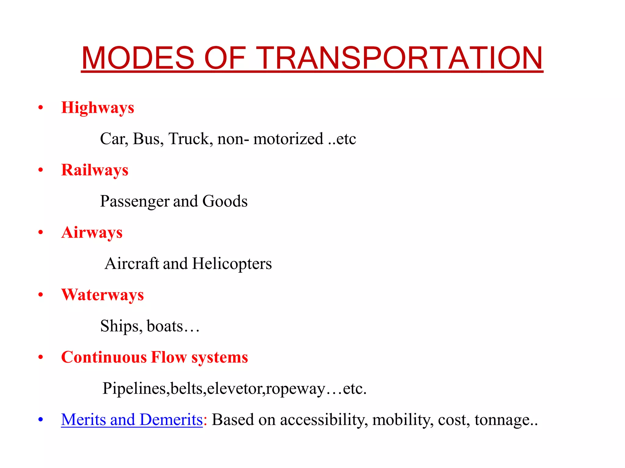
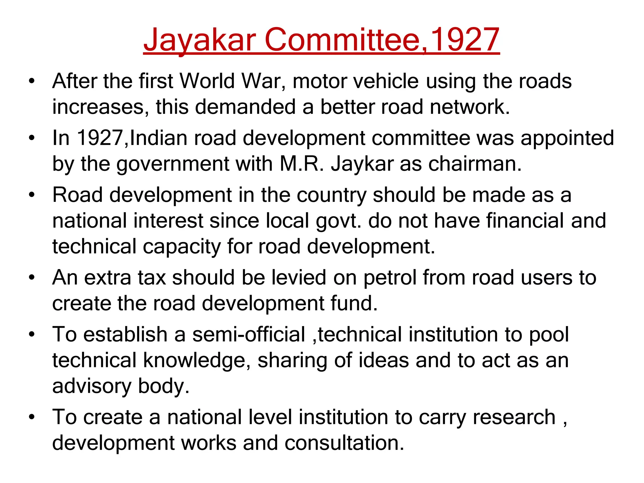
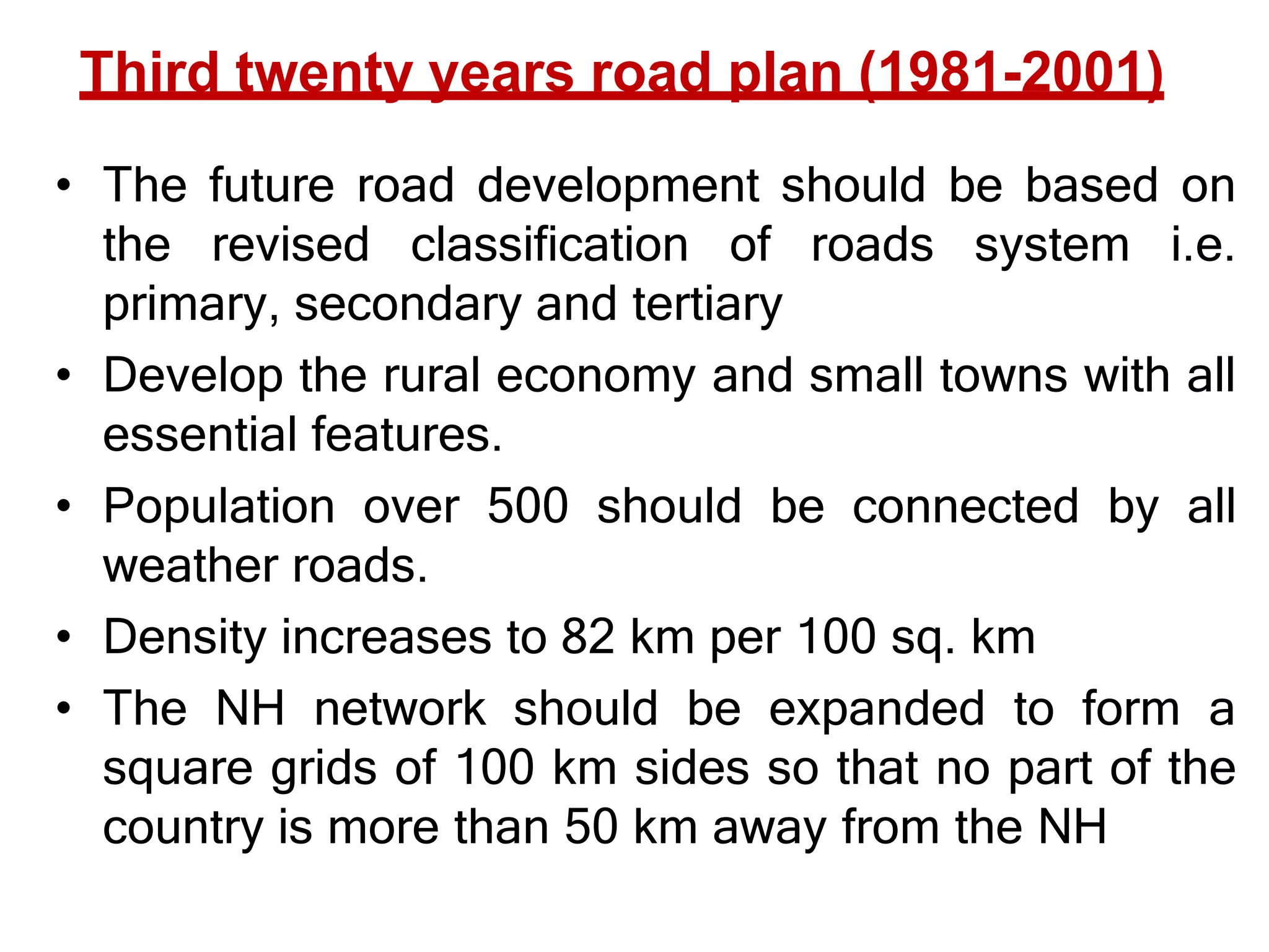
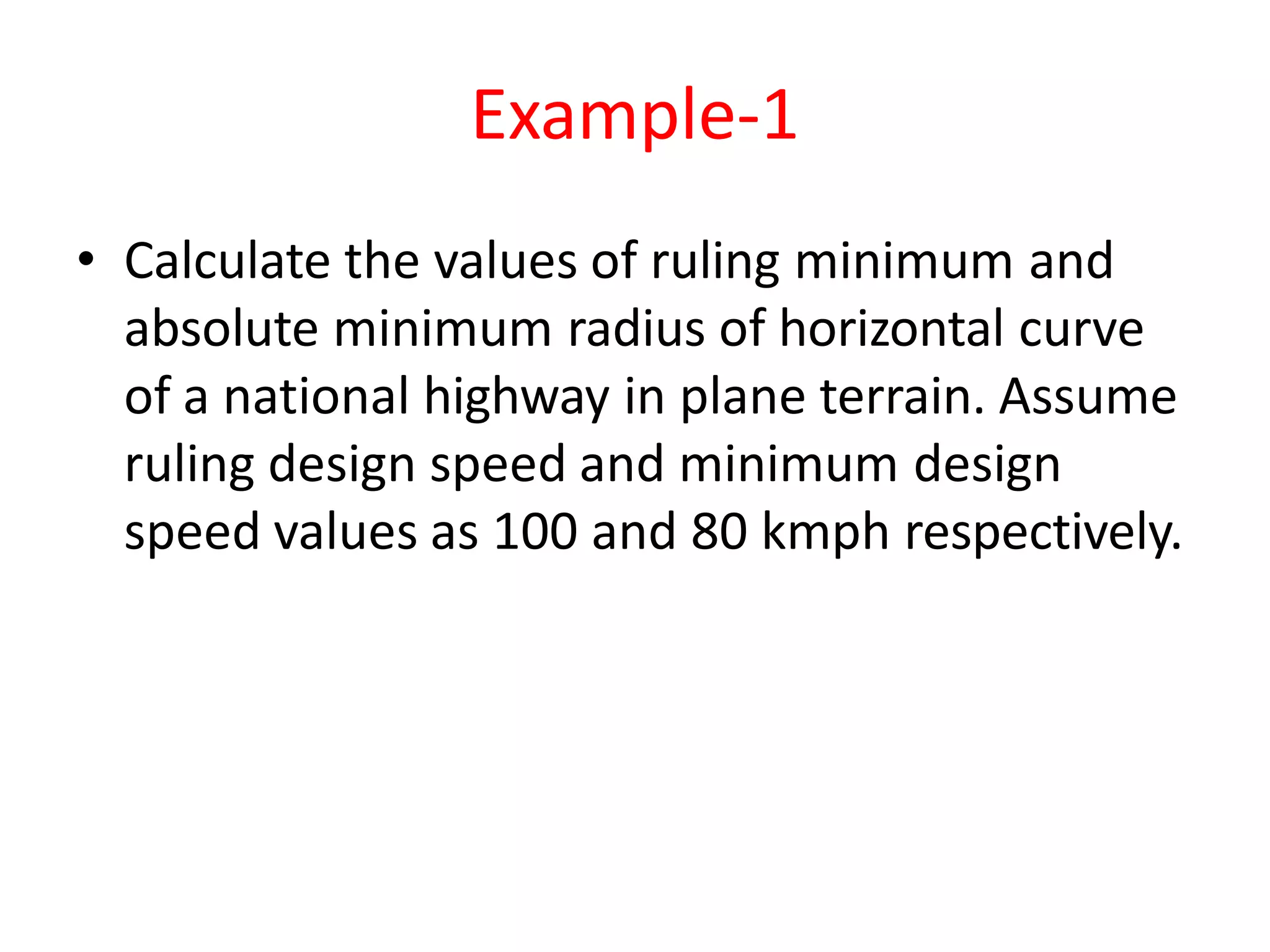
This document provides an overview of transportation engineering and highway development and planning in India. It discusses the different modes of transportation including road, rail, air, and waterways. It then focuses on highways, describing their historical development in India through committees and plans over the 20th century to expand and classify the road network. These included the Jayakar Committee (1927), Central Road Fund (1929), Indian Roads Congress (1934), and three national road development plans from 1943-2001. The document also covers highway alignment, classification of highways, and urban road classification.
DAVV IET_ TraNSPORTATION [PPT LECTURES ALL 501.pptxprtaap1
(Established by the Government of India under NITSER Act,)
P.O. ICHCHHANATH, SURAT-395 007, GUJARAT, INDIA
Website: http://www.svnit.ac.in
Advt No. Estt. /2022/Gr_A1/2002 Date: October 17, 2022
RECRUITMENT FOR NON-TEACHING POSITIONS
Sardar Vallabhbhai National Institute of Technology Surat (SVNIT) was established by the
Government of India by an Act of Parliament, offering UG, PG and Ph.D. Programs in Engineering/
Technology and Sciences. The Institute is in search of bright, dynamic, experienced, qualified, and
suitable Indian Nationals to cater the Institute’s requirement. The Institute invites online
applications for the following Non-teaching positions on direct recruitment in various departments/
sections of the Institute:
Sl.
No
Name of the Post (s)
& Specialization/
Relevant Field
Pay Level
(as per 7 CPC)
No of Vacant Posts* Total* Upper
Age
Limit
UR SC ST OBCNCL
EWS
1 Librarian Pay Level 14
[PB-4 & GP Rs
10000]
1 - - - - 1 56
2 Scientific Officer /
Technical Officer
(MIS)
Pay Level 10
[PB-3 & GP Rs
5400]
1 - - - - 1 35
3 Executive Engineer
(Civil-01, Electrical-
01)
Pay Level 10
[PB-3 & GP Rs
5400]
2 - - - - 2 35
Total 4 0 0 0 0 4
*One post will be filled up from the identified person with benchmark disabilities, if found suitable
The eligibility criteria for the above posts is as per Recruitment Rules of NITs (2019) and as
updated from time to time by Ministry of Education, Govt. of India. For details regarding the
online Application Form, Educational Qualifications, Experience, other requirements and terms &
conditions for these positions, please visit the Institute website http://www.svnit.ac.in. The
number of Posts may vary at the time of final selection / recruitment.
The recruitment notice for the post advertised vide advertisement no. Estt./2021/Gr_A/3051
dated 02.03.2021 & Estt./2021/2021/EE/678 dated 07.06.2021 for which the recruitment process
has not been completed is cancelled vide Notice No.E/Rect.(2021)/1165 dated 14.10.2022. The
interested applicant who has applied earlier may apply afresh.
The interested candidates may apply online through the Institute website http://www.svnit.ac.in
and send the filled in downloaded online application form duly singed alongwith self-attested
documents viz. relevant testimonials, certificates, payment receipts etc. by speed/ registered
posts to the Deputy Registrar (Establishment), Sardar Vallabhbhi National Institute of
Technology, Ichchhanath, Dumas Road, Surat – 395 007, Gujarat, The applications received
through any other mode shall not be accepted and summarily rejected. The last date for
submission of online application is December 02, 2022 till 5.00 p.m. and receipt of
downloaded signed completed application at SVNIT Surat is December 12, 2022.
-sd/-
REGISTRAR
1
(Established by the Government of India under NITSER Act,)
P.O. ICHCHHANATH, SURAT-395 007, GUJARAT, INDIA
Website: http://www.svnit.ac.in
Advt No. Estt. /2022/Gr_A1/2002 Date: October 17, 2022
RECRUITMENT FOR NON-TEACHING P
Highway planning and alignment: Different modes of transportation – historical Development of road construction- Highway Development in India –Classification of roads- Road pattern
– Highway planning in India- Highway alignment - Engineering Surveys for alignment – Highway Project- Important Transport/Highway related agencies in India. PMGSY project.
Introduction about IRC, NRRDA
Transportation engineering, primarily involves planning, design, construction, maintenance, and operation of transportation facilities. The facilities support air, highway, railroad, pipeline, water, and even space transportation.
CBSE Class X-Geo(7) : Lifelines of National Economy Chapter in an easy and simple way, for everyone to understand. For all students and who have have slow pace also.
Sachpazis:Terzaghi Bearing Capacity Estimation in simple terms with Calculati...Dr.Costas Sachpazis
Terzaghi's soil bearing capacity theory, developed by Karl Terzaghi, is a fundamental principle in geotechnical engineering used to determine the bearing capacity of shallow foundations. This theory provides a method to calculate the ultimate bearing capacity of soil, which is the maximum load per unit area that the soil can support without undergoing shear failure. The Calculation HTML Code included.
Student information management system project report ii.pdfKamal Acharya
Our project explains about the student management. This project mainly explains the various actions related to student details. This project shows some ease in adding, editing and deleting the student details. It also provides a less time consuming process for viewing, adding, editing and deleting the marks of the students.
About
Indigenized remote control interface card suitable for MAFI system CCR equipment. Compatible for IDM8000 CCR. Backplane mounted serial and TCP/Ethernet communication module for CCR remote access. IDM 8000 CCR remote control on serial and TCP protocol.
• Remote control: Parallel or serial interface.
• Compatible with MAFI CCR system.
• Compatible with IDM8000 CCR.
• Compatible with Backplane mount serial communication.
• Compatible with commercial and Defence aviation CCR system.
• Remote control system for accessing CCR and allied system over serial or TCP.
• Indigenized local Support/presence in India.
• Easy in configuration using DIP switches.
Technical Specifications
Indigenized remote control interface card suitable for MAFI system CCR equipment. Compatible for IDM8000 CCR. Backplane mounted serial and TCP/Ethernet communication module for CCR remote access. IDM 8000 CCR remote control on serial and TCP protocol.
Key Features
Indigenized remote control interface card suitable for MAFI system CCR equipment. Compatible for IDM8000 CCR. Backplane mounted serial and TCP/Ethernet communication module for CCR remote access. IDM 8000 CCR remote control on serial and TCP protocol.
• Remote control: Parallel or serial interface
• Compatible with MAFI CCR system
• Copatiable with IDM8000 CCR
• Compatible with Backplane mount serial communication.
• Compatible with commercial and Defence aviation CCR system.
• Remote control system for accessing CCR and allied system over serial or TCP.
• Indigenized local Support/presence in India.
Application
• Remote control: Parallel or serial interface.
• Compatible with MAFI CCR system.
• Compatible with IDM8000 CCR.
• Compatible with Backplane mount serial communication.
• Compatible with commercial and Defence aviation CCR system.
• Remote control system for accessing CCR and allied system over serial or TCP.
• Indigenized local Support/presence in India.
• Easy in configuration using DIP switches.
Hybrid optimization of pumped hydro system and solar- Engr. Abdul-Azeez.pdffxintegritypublishin
Advancements in technology unveil a myriad of electrical and electronic breakthroughs geared towards efficiently harnessing limited resources to meet human energy demands. The optimization of hybrid solar PV panels and pumped hydro energy supply systems plays a pivotal role in utilizing natural resources effectively. This initiative not only benefits humanity but also fosters environmental sustainability. The study investigated the design optimization of these hybrid systems, focusing on understanding solar radiation patterns, identifying geographical influences on solar radiation, formulating a mathematical model for system optimization, and determining the optimal configuration of PV panels and pumped hydro storage. Through a comparative analysis approach and eight weeks of data collection, the study addressed key research questions related to solar radiation patterns and optimal system design. The findings highlighted regions with heightened solar radiation levels, showcasing substantial potential for power generation and emphasizing the system's efficiency. Optimizing system design significantly boosted power generation, promoted renewable energy utilization, and enhanced energy storage capacity. The study underscored the benefits of optimizing hybrid solar PV panels and pumped hydro energy supply systems for sustainable energy usage. Optimizing the design of solar PV panels and pumped hydro energy supply systems as examined across diverse climatic conditions in a developing country, not only enhances power generation but also improves the integration of renewable energy sources and boosts energy storage capacities, particularly beneficial for less economically prosperous regions. Additionally, the study provides valuable insights for advancing energy research in economically viable areas. Recommendations included conducting site-specific assessments, utilizing advanced modeling tools, implementing regular maintenance protocols, and enhancing communication among system components.
Overview of the fundamental roles in Hydropower generation and the components involved in wider Electrical Engineering.
This paper presents the design and construction of hydroelectric dams from the hydrologist’s survey of the valley before construction, all aspects and involved disciplines, fluid dynamics, structural engineering, generation and mains frequency regulation to the very transmission of power through the network in the United Kingdom.
Author: Robbie Edward Sayers
Collaborators and co editors: Charlie Sims and Connor Healey.
(C) 2024 Robbie E. Sayers
COLLEGE BUS MANAGEMENT SYSTEM PROJECT REPORT.pdfKamal Acharya
The College Bus Management system is completely developed by Visual Basic .NET Version. The application is connect with most secured database language MS SQL Server. The application is develop by using best combination of front-end and back-end languages. The application is totally design like flat user interface. This flat user interface is more attractive user interface in 2017. The application is gives more important to the system functionality. The application is to manage the student’s details, driver’s details, bus details, bus route details, bus fees details and more. The application has only one unit for admin. The admin can manage the entire application. The admin can login into the application by using username and password of the admin. The application is develop for big and small colleges. It is more user friendly for non-computer person. Even they can easily learn how to manage the application within hours. The application is more secure by the admin. The system will give an effective output for the VB.Net and SQL Server given as input to the system. The compiled java program given as input to the system, after scanning the program will generate different reports. The application generates the report for users. The admin can view and download the report of the data. The application deliver the excel format reports. Because, excel formatted reports is very easy to understand the income and expense of the college bus. This application is mainly develop for windows operating system users. In 2017, 73% of people enterprises are using windows operating system. So the application will easily install for all the windows operating system users. The application-developed size is very low. The application consumes very low space in disk. Therefore, the user can allocate very minimum local disk space for this application.
Saudi Arabia stands as a titan in the global energy landscape, renowned for its abundant oil and gas resources. It's the largest exporter of petroleum and holds some of the world's most significant reserves. Let's delve into the top 10 oil and gas projects shaping Saudi Arabia's energy future in 2024.
Courier management system project report.pdfKamal Acharya
It is now-a-days very important for the people to send or receive articles like imported furniture, electronic items, gifts, business goods and the like. People depend vastly on different transport systems which mostly use the manual way of receiving and delivering the articles. There is no way to track the articles till they are received and there is no way to let the customer know what happened in transit, once he booked some articles. In such a situation, we need a system which completely computerizes the cargo activities including time to time tracking of the articles sent. This need is fulfilled by Courier Management System software which is online software for the cargo management people that enables them to receive the goods from a source and send them to a required destination and track their status from time to time.
Vaccine management system project report documentation..pdfKamal Acharya
The Division of Vaccine and Immunization is facing increasing difficulty monitoring vaccines and other commodities distribution once they have been distributed from the national stores. With the introduction of new vaccines, more challenges have been anticipated with this additions posing serious threat to the already over strained vaccine supply chain system in Kenya.
Vaccine management system project report documentation..pdf
Transportation Engg.pptx
1. Civil Engineering Department
Noida International University (NIU)
Greater Noida
Module-1
Highway Development And Planning
TRANSPORTATION ENGINEERING
PCC-CE307
2. Transportation engineering
• Transportation engineering is the
application of technology and scientific
principles to the planning, functional design,
operation and management of facilities for
any mode of transportation in order to
provide for the safe, efficient, rapid,
comfortable, convenient, economical, and
environmentally compatible movement of
people and goods from one place to other.
4. MODES OF TRANSPORTATION
• Highways
Car, Bus, Truck, non- motorized ..etc
• Railways
Passenger and Goods
• Airways
Aircraft and Helicopters
• Waterways
Ships, boats…
• Continuous Flow systems
Pipelines,belts,elevetor,ropeway…etc.
• Merits and Demerits: Based on accessibility, mobility, cost, tonnage..
5. Airways
• Fastest among all other modes
• More comfortable
• Time saving
• Uneconomical
Waterways
• slowest among all other modes
• It needs minimum energy to haul unit load
through unit distance.
• This can be possible between ports on the sea
routes or along the river
• economical
6. Railways
• The transportation along the railways track
could be advantageous by railways between
the stations both for the passengers and
goods, particularly for long distance.
• It depends upon the road transport i.e. road
could serve as a feeder system.
• Energy require to haul a unit load through
unit distance by the railway is only ¼ to 1/5
of that required by road.
• Safety
7. Highways
• It gives the maximum service to one and all
• It gives maximum flexibility for travel with reference
to route, direction, time and speed of travel
• It provide door to door service
• Other modes are depend on it
• It requires small investment for the government
• Motor vehicles are cheaper than other carriers like
rail locomotive and wagons
• It saves the time for short distance
• High degree of accident due to flexibility of
movement
8. Scope of highway engineering
• Development, planning and location
• Highway design, geometric and structure
• Traffic performance and its control
• Materials, construction and maintenance
• Economic, finance and administration
9. ROLE /IMPACT OF TRANSPORTATION
• Economic Development
• Social Development
• Spatial Development
• Cultural Development
• Political Development
10. Characteristics of road transport
• Roads are used by various types of road vehicles,
like passenger cars, buses, trucks, pedal cycle and
animal drawn vehicle.
• It requires a relatively small investment for the
government.
• It offers a complete freedom to road users to
transfer the vehicle from one lane to another and
from one road to another according to need and
convenience.
• Speed and movement is directly related with the
severity of accident.
• Road transport is the only means of transport that
offers itself to the whole community alike.
11. HISTORICAL DEVELOPMENT OF ROAD
CONSTRUCTION
• Oldest mode
Foot paths- animal ways, cart path……..
• As civilization evolved the need for transportation
increased
ROMAN ROAD-(500 B.C.)
They were built straight regardless of gradient
They were built after the soft soil was removed and
a hard stratum was reached.
Thickness varies from 0.75 m to 1.2m
14. Other oldest road transport are
• Tresaguet construction
• Metcalf construction
• Telford construction
• Mecadam construction
15. Indian Roads
• India has a large road network of over 3.314
million kilometers of roadways (2.1 million
miles), making it 3rd largest road network in the
world.
• At 0.66 km of highway per square kilometer of
land the density of India’s highway network is
higher than that of the United States (0.65) and
far higher than that of China's (0.16) or Brazil's
(0.20).
16. Highway Development in India
• Jayakar Committee (1927)
• Central Road Fund (1929)
• Indian Roads Congress (IRC), 1934
• Central Road Research Institute (CRRI), 1950
• Motor vehicle act (1936)
• National Highway Authority of India (NHAI),1995
• First twenty year road plan ( 1943-61 )
• Second twenty year road plan ( 1961-81 )
• Highway Research board ( 1973 )
• National Transport Policy committee ( 1978 )
• Third twenty year road plan ( 1981-2001 )
17. Jayakar Committee,1927
• After the first World War, motor vehicle using the roads
increases, this demanded a better road network.
• In 1927,Indian road development committee was appointed
by the government with M.R. Jaykar as chairman.
• Road development in the country should be made as a
national interest since local govt. do not have financial and
technical capacity for road development.
• An extra tax should be levied on petrol from road users to
create the road development fund.
• To establish a semi-official ,technical institution to pool
technical knowledge, sharing of ideas and to act as an
advisory body.
• To create a national level institution to carry research ,
development works and consultation.
18. Central road fund
• It was formed on 1st march 1929
• The consumers of petrol were charged an extra
leavy of 2.64 paisa per litre of petrol to built up
this road development fund.
• From this 20% of annual reveneu is to be retain
as a central reveneu for research and
experimental work expenses..etc
• Balance 80% is allowed by central govt. to
various states based on actual petrol
consumption or revenue collected.
19. Central Road Fund , 1929
CRF Act , 2000
Distribution of 100% cess on petrol as follows:
57.5% for NH
30% for SH
12.5% for safety works on rail-Road crossing.
50% cess on diesel for Rural Road development
MORTH
20. Indian Roads Congress, 1934
• Central semi official body known as IRC was formed in
1934.
• To provide national forum for regular pooling of
experience and ideas on matters related to construction
and maintenance of highways.
• It is a active body controlling the specification,
standardization and recommendations on materials,
design of roads and bridges.
• It publishes journals, research publications and standard
specifications guide lines.
• To provide a platform for expression of professional
opinion on matters relating to roads and road transport.
21. Motor vehicle act
• It was formed in 1939
• To regulate the road traffic in the form of
traffic laws, ordinances and regulations.
• Three phases primarily covered are
control of driver, vehicle ownership and
vehicle operation
• It was revised on 1988
22. Central road research institute(1950)
engaged in carrying out research and development
projects.
design, construction and maintenance of roads and
runways, traffic and transportation planning of mega
and medium cities, management of roads in different
terrains,
Improvement of marginal materials.
Utilization of industrial waste in road construction.
Landslide control.
Ground improvements, environmental pollution.
Road traffic safety.
23. Ministry of Road Transport & Highways
• Planning, development and maintenance of
National Highways in the country.
• Extends technical and financial support to State
Governments for the development of state roads
and the roads of inter-state connectivity and
economic importance.
• Evolves standard specifications for roads and
bridges in the country.
• It stores the data related to technical knowledge
on roads and bridges.
24. Highway Research Board
• To ascertain the nature and extent of
research required
• To correlate research information from
various organisation in India and abroad.
• To collect and correlation services.
• To collect result on research
• To channelise consultative services
25. Classification of Highways
Depending on weather
All weather roads
Fair weather roads
Depending the type of Carriage way
Paved roads(WBM)
Unpaved roads(earth road or gravel road)
Depending upon the pavement surface
Surfaced roads(bituminous or cement concrete
road)
Un surfaced roads
26. Based on the Traffic Volume
Heavy
Medium
Light
Based on Load or Tonnage
Class 1 or Class 2 etc or Class A , B etc Tonnes per
day
Based on location and function ( Nagpur road plan )
National highway (NH)
State highway (SH)
Major district road (MDR)
Other district road (ODR)
Village road (VR)
Classification of Highways
27. Based on modified system of
Highways classification
• Primary
Expressways
National Highways
• Secondary
SH
MDR
• Tertiary
ODR
VR
28. Expressways
• Heavy traffic at high speed (120km/hr)
• Land Width (90m)
• Full access control
• Connects major points of traffic generation
• No slow moving traffic allowed
•No loading, unloading,
parking.
The Mumbai-Pune Expressway as seen
from Khandala
29. National Highways
• NH are the main highways running through the length and
breadth of India, connecting major parts,foreign
highways,capital of large states and large industrial and
tourist centres including roads required for strategic
movements for the defence of India.
• The national highways have a total length of 70,548 kms.
Indian highways cover 2% of the total road network of India
and carry 40% of the total traffic.
• The highway connecting Delhi-Ambala-Amritsar is denoted
as NH-1, whereas a bifurcation of this highway beyond
Jalandar to Srinagar and Uri is denoted NH-1-A
• The longest highway in India is NH7 which stretches from
Varansi in Uttar Pradesh to Kanyakumari in the southern
most point of Indian mainland.
30. National Highways cont …
• The shortest highway is NH47A which stretches
from Ernakulam to Kochi and covers total length of
4 Kms.
• Golden Quadrilateral – (5,846 Kms) connecting Delhi-
Kolkata-Chennai-Mumbai
NH-2 Delhi- Kol (1453 km)
NH 4,7&46 Che-Mum (1290km )
NH5&6 Kol- Che (1684 m)
NH 8 Del- Mum (1419 km)
31. State Highways
• They are the arterial roads of a state,
connecting up with the national highways of
adjacent states, district head quarters and
important cities within the state.
• Total length of all SH in the country is
1,37,119 Kms.
• Speed 80 kmph
32. Major District Roads
• Important roads with in a district serving
areas of production and markets ,
connecting those with each other or with
the major highways.
• India has a total of 4,70,000 kms of MDR.
• Speed 60-80kmph
33. Other district roads
serving rural areas of production and providing
them with outlet to market centers or other
important roads like MDR or SH.
Speed 50-60kmph
Village roads
• They are roads connecting villages or group of
villages with each other or to the nearest road of a
higher category like ODR or MDR.
• India has 26,50,000 kms of ODR+VR out of the
total 33,15,231 kms of all type of roads.
• Speed-40-50kmph
34. Urban Road Classification
• Arterial Roads
• Sub Arterial
• Collector
• Local Street
• Cul-de-sac
• Pathway
• Driveway
35. ARTERIAL
• No frontage access, no standing vehicle,
very little cross traffic.
• Design Speed : 80km/hr
• Land width : 50 – 60m
• Divided roads with full or partial parking
• Pedestrian allowed to walk only at
intersection
36. SUB ARTERIAL ROAD
• Bus stops but no standing vehicle.
• Less mobility than arterial.
• Spacing for CBD
• Design speed
• Land width
: 0.5km
: 60 km/hr
: 30 – 40 m
37. Collector Street
• Collects and distributes traffic from local
streets
• Provides access to arterial roads
• Located in residential, business and
industrial areas.
• Full access allowed.
• Parking permitted.
• Design speed : 50km/hr
• Land Width : 20-30m
38. Local Street
• Design Speed : 30km/hr.
• Land Width : 10 – 20m.
• Primary access to residence, business or
other abutting property
• Less volume of traffic at slow speed
• Unrestricted parking, pedestrian
movements. (with frontage access, parked
vehicle, bus stops and no waiting
restrictions)
39. CUL–DE- SAC
• Dead End Street with only one entry
access for entry and exit.
• Recommended in Residential areas
40. Driveway
• A driveway is a type of private road for local
access to one or a small group of structures, and
is owned and maintained by an individual or
group.
• Driveways are commonly used as paths to
private garages, fuel stations, or houses
41. Road Patterns
• Rectangular or Block patterns
• Radial or Star block pattern
• Radial or Star Circular pattern
• Radial or Star grid pattern
• Hexagonal Pattern
• Minimum travel Pattern
42. First 20-years road plan(1943-63)
• The conference of chief engineer held at Nagpur in
1943 finalized the first 20-years road development
plan for India called Nagpur road plan
• Road network was classified into five categories.
• The responsibility of construction maintenance of NH
was assign to central govt.
• The target road length was 5,32,700 km at the end of
1961.
• Density of about 16km of road length per 100 sq. km
area would be available in the country by the year
1963.
43. First 20-years road plan cont…
• The formulae were based on star and grid
pattern of road network.
• An allowance of 15% is provided for
agricultural industrial development during the
next 20-years
• The length of railway track in the area was
also consider in deciding the length of first
category road. The length or railway track is
directly subtracted from the estimated road
length of metalled roads.
44. Second 20-years road plan(1961-81)
• It was initiated by the IRC and was finalised in
1959 at the meeting of chief engineers.
• It is known as the Bombay road plan.
• The target road length was almost double that
of Nagpur road plan i.e. 10,57,330 km.
• Density about 32 km per 100 sq. km. and an
outlay of 5200 crores
• Every town with population above 2000 in
plans and above 1000 in semi hill area and
above 500 in hilly area should be connected
by metalled road
45. Second 20-years road plan cont…
• the maximum distance from any place in a
semi develop area would be 12.8 km from
metalled road and 4.8 from any road
• Expressways have also been considered in
this plan and 1600km of length has been
included in the proposed target NH
• Length of railway track is considered
independent of road system
• 5% are to be provided for future development
and unforeseen factor
46. Third twenty years road plan (1981-2001)
• The future road development should be based on
the revised classification of roads system i.e.
primary, secondary and tertiary
• Develop the rural economy and small towns with all
essential features.
• Population over 500 should be connected by all
weather roads.
• Density increases to 82 km per 100 sq. km
• The NH network should be expanded to form a
square grids of 100 km sides so that no part of the
country is more than 50 km away from the NH
47. Third twenty years road plan cont…
• Expressway should be constructed along major
traffic corridors
• All towns and villages with population over 1500
should be connected by MDR and villages with
population 1000-1500 by ODR.
• Road should be built in less industrialized areas to
attract the growth of industries
• The existing roads should be improved by rectifying
the defects in the road geometry, widening, riding
quality and strengthening the existing pavement to
save vehicle operation cost and thus to conserve
energy
49. Highway alignment
• The position or lay out of centre line of the highway
on the ground is called the alignment.
• It includes straight path, horizontal deviation and
curves.
• Due to improper alignment , the disadvantages are,
Increase in construction
Increase in maintenance cost
Increase in vehicle operation cost
Increase in accident cost
• Once the road is aligned and constructed, it is not
easy to change the alignment due to increase in
cost of adjoining land and construction of costly
structure.
50.
51.
52. Short
Easy
Safe
Economical
• Short- desirable to have a short alignment between two
terminal stations.
• Easy- easy to construct and maintain the road with minimum
problem also easy for operation of vehicle.
• Safe- safe enough for construction and maintenance from
the view point of stability of natural hill slope, embankment
and cut slope also safe for traffic operation.
• Economical- total cost including initial cost, maintenance
cost and vehicle operation cost should be minimum.
Requrements of highway alignment
53. Factors controlling alignment
Obligatory points
Traffic
Geometric design
Economics
Other considerations
Additional care in hill roads
Stability
Drainage
Geometric standards of hill roads
Resisting length
54. Factors controlling alignment cont...
Obligatory points
Obligatory points through which alignment is to pass
Examples:-bridge site, intermediate town , Mountain pass etc…
Obligatory points through which alignment should not
pass.
Examples:-religious places, costly structure, unsuitable land etc…
Traffic
• origin and destination survey should be carried out in the
area and the desire lines be drawn showing the trend of
traffic flow.
• New road to be aligned should keep in view the desired lines,
traffic flow patterns and future trends.
55. Geometric design
• Design factors such as gradient ,radius of curve and sight
distance also govern the final alignment of the highway.
• Gradient should be flat and less than the ruling gradient or
design gradient.
• Avoid sudden changes in sight distance, especially near
crossings
• Avoid sharp horizontal curves
• Avoid road intersections near bend
Economy
• Alignment finalised based on total cost including initial cost,
maintenance cost and vehicle operation cost.
Other consideration
• Drainage consideration, political consideration
• Surface water level, high flood level
• Environmental consideration
56. Topographical control points
• The alignment, where possible should avoid passing
through
Marshy and low lying land with poor drainage
Flood prone areas
Unstable hilly features
Materials and constructional features
Deep cutting should be avoided
Earth work is to be balanced; quantities for filling and
excavation
Alignment should preferably be through better soil area
to minimize pavement thickness
Location may be near sources of embankment and
pavement materials
57. stability
• A common problem in hilly roads is land sliding
• The cutting and filling of the earth to construct the roads on
hilly sides causes steepening of existing slope and affect its
stability.
Drainage
• Avoid the cross drainage structure
• The number of cross drainage structure should be minimum.
Geometric standard of hilly road
• Gradient, curve and speed
• Sight distance, radius of curve
Resisting length
• The total work to be done to move the loads along the route
taking horizontal length, the actual difference in level between
two stations and the sum of the ineffective rise and fall in
excess of floating gradient. Should kept as low as possible.
58. Before a highway alignment is finalised in highway
project, the engineering survey are to be carried out.
The various stages of engineering surveys are
Map study (Provisional alignment Identification)
Reconnaissance survey
Preliminary survey
Final location and detailed surveys
Engineering Surveys for Highway locations
59. MAP STUDY
• From the map alternative routes can be suggested
in the office, if the topographic map of that area is
available.
• The probable alignment can be located on the map
from the fallowing details available on the map.
Avoiding valleys, ponds or lake
Avoiding bend of river
If road has to cross a row of hills, possibility of
crossing through mountain pass.
• Map study gives a rough guidance of the routes to
be further surveyed in the field
60. RECONNAISSANCE SURVEY
• To confirm features indicated on map.
• To examine the general character of the area in field for
deciding the most feasible routes for detailed studies.
• A survey party may inspect along the proposed alternative
routes of the map in the field with very simple instrument
like abney level, tangent clinometer, barometer etc…. To
collect additional details.
• Details to be collected from alternative routes during this
survey are,
Valleys, ponds, lakes, marshy land, hill, permanent
structure and other obstruction.
Value of gradient, length of gradient and radius of curve.
61. RECONNAISSANCE SURVEY cont..
Number and type of cross drainage structures.
High Flood Level (HFL)
Soil Characteristics.
Geological features.
source of construction materials- stone quarries, water
sources.
• Prepare a report on merits and demerits of different
alternative routs.
• As a result a few alternate alignments may be chosen for
further study based on practical considerations observed
at the site.
62. Preliminary survey
Objective of preliminary survey are:
• To survey the various alternative alignments proposed after
the reconnaissance and to collect all the necessary physical
information and detail of topography, drainage and soil.
• To compare the different proposals in view of the
requirements of the good alignment.
• To estimate quantity of earthwork materials and other
construction aspect and to workout the cost of the alternate
proposals.
Methods of preliminary survey:
a) Conventional approach-survey party carries out surveys
using the required field equipment, taking measurement,
collecting topographical and other data and carrying out soil
survey.
63. Preliminary survey cont…
• Longitudinal and cross sectional profile.
: 100 – 200m
: 50m
: 30m
Plain Terrain`
Rolling Terrain
Hilly Terrain
• Other studies
Drainage, Hydrological survey, soil survey, Traffic and
Material survey.
b) Modern rapid approach-
By Aerial survey taking the required aerial photographs for
obtaining the necessary topographic and other maps
including details of soil and geology.
• Finalise the best alignment from all considerations by
comparative analysis of alternative routes.
64. Final location and detailed survey
• The alignment finalised at the design office after the
preliminary survey is to be first located on the field by
establishing the centre line.
Location survey:
• Transferring the alignment on to ground.
• This is done by transit theodolite.
• Major and minor control points are established on the
ground and centre pegs are driven, checking the
geometric design requirements.
• Centre line stacks are driven at suitable intervals, say 50m
interval in plane and rolling terrains and 20m in hilly
terrain.
65. Final location and detailed survey cont..
Detailed survey:
• Temporary bench marks are fixed at intervals of about 250m
and at all drainage and under pass structure.
• Earthwork calculations and drainage details are to be workout
from the level books.
• Cross sectional levels are taken at intervals of 50-100m in
Plane terrain, 50-75m in Rolling terrain, 50m in built-up area,
20m in Hill terrain.
• Detail soil survey is to be carried out.
• CBR value of the soils along the alignment may be determined
for design of pavement.
• The data during detailed survey should be elaborate and
complete for preparing detailed plans, design and estimates of
project.
66. Drawing and Report
Key map
Index map
Preliminary survey plans
Detailed plan and longitudinal section
Detailed cross section
Land acquisition plans
Drawings of cross drainage and other retaining
structures
Drawings of road intersections
Land plans showing quarries etc
67. New highway project
• Map study
• Reconnaissance survey
• Preliminary survey
• Location of final alignment
• Detailed survey
• Material survey
• Geometric and structural design
• Earth work
• Pavement construction
• Construction controls
69. Module -2
Highway Geometric Design
Civil Engineering Department
Noida International University (NIU)
Greater Noida
TRANSPORTATION ENGINEERING
PCC-CE307
70. Importance of geometric design
• The geometric design of a highway deals with the
dimensions and layout of visible features of the
highway such as alignment, sight distance and
intersection.
• The main objective of highway design is to provide
optimum efficiency in traffic operation with maximum
safety at reasonable cost.
• Geometric design of highways deals with following
elements :
Cross section elements
Sight distance considerations
Horizontal alignment details
Vertical alignment details
Intersection elements
71. Design Controls and criteria
• Design speed
• Topography
• Traffic factors
• Design hourly volume and capacity
•Environmental and other factors
Design speed
• In India different speed standards have been assigned
for different class of road
• Design speed may be modified depending upon the
terrain conditions.
72. topography
• Classified based on the general slope of the country.
Plane terrain- <10%
Rolling terrain- 10-25%
Mountainous terrain- 25-60%
Steep terrain- >60%
Traffic factor
• Vehicular characteristics and human characteristics of road
users.
• Different vehicle classes have different speed and
acceleration characteristics, different dimensions and
weight .
• Human factor includes the physical, mental and
psychological characteristics of driver and pedestrian.
73. Design hourly volume and capacity
• Traffic flow fluctuating with time
• Low value during off-peak hours to the highest
value during the peak hour.
• It is uneconomical to design the roadway for peak
traffic flow.
Environmental factors
Aesthetics
Landscaping
Air pollution
Noise pollution
74. Pavement surface characteristics
Pavement surface depend on the type of
pavement which is decided based on the,
• Availability of material
• Volume and composition of traffic
• Soil subgrade
• Climatic condition
• Construction facility
• Cost consideration
The important surface characteristics are:
Friction
Pavement unevenness
Light reflecting characteristics
Drainage of surface water
75. friction
• Skidding: when the path travelled along the road surface is
more than the circumferential movement of the wheels
due to their rotation.
• Slipping: when a wheel revolves more than the
corresponding longitudinal movement along the road.
Factors affecting the friction or skid resistance
• Types of pavement surface
• Roughness of pavement
• Condition of the pavement: wet or dry
• Type and condition of tyre
• Speed of the vehicle
• Brake efficiency
• Load and tyre pressure
• Temperature of tyre and pavement
76. Smooth and worn out tyres offer higher friction
factor on dry pavement but new tyre with good threds
gives higher friction factor on wet pavement
IRC recommended the longitudinal co-
efficient of friction varies 0.35 to 0.4 and
lateral co-efficient of friction of 0.15
77. Pavement unevenness
• Higher operating speed are possible on even surface than
uneven surface.
• It affects,
Vehicle operation cost
Comfort and safety
Fuel consumption
Wear and tear of tyres and other moving parts
• It is commonly measure by an equipment call “Bump
Integrator”
• Bump integrator is the cumulative measure of vertical
undulations of the pavement surface recorded per unit
horizontal length.
• 250 cm/km for a speed of 100kmph and more than 350
cm/km considered very unsatisfactory even at speed of 50
kmph.
78. Unevenness of pavement surface may be caused by
In adequate compaction of the fill, subgrade
and pavement layers.
Un-scientific construction practices including
the use of boulder stones and bricks as soiling
course over loose subgrade soil.
Use of inferior pavement material.
Improper surface and subsurface drainage.
Improper construction machinery.
Poor maintenance
79.
80. Light reflecting characteristics
• Night visibility very much depends upon the light
reflecting characteristics of the pavement surface
• The glare caused by the reflection of head light is
high on wet pavement surface than on dry
pavement particularly in case of black top
pavement or flexible pavement.
• Light colored or white pavement or rigid
pavement surface give good visibility at night
particularly during the rain, and produces glare or
eye strain during bright sunlight.
81. Highway cross section elements
• Carriageway
• Shoulder
• Roadway width
• Right of way
• Building line
• Control line
• Median
• Camber/ cross slope
• Crown
• Side slope
• Kerb
• Guard rail
• Side drain
• Other facilities
82. Carriageway:
• It is the travel way which is used for movement of
vehicle, it takes the vehicular loading .
• It may be cement concrete road or bituminous
pavement.
• Width of carriageway is determined on the basis
of the width of the vehicle and the minimum side
clearance for safety.
• As per IRC specification, the maximum width of
vehicle is 2.44m,minimum clearance of 0.68 in
case of single lane and 1.02m in case of double
lane.
83. WIDTH OF CARRIAGEWAY
SL. NO. Class of road Width of carriageway in ‘m’
1 Single lane 3.75
2 Two lane without raised kerbs 7.0
3 Two lane with raised kerbs 7.5
4 Intermediate lane 5.5
5 Multilane pavement 3.5/lane
WIDTH OF ROADWAY OF VARIOUS CLASSES OF ROADS
SL. No. Road classification Roadway wisth
Plane and rolling terrain Mountainous and steep
terrain
1 NH & SH
a) Single lane
b) two lane
12
12
6.25
6.25
2 MDR
a) Single lane
b) two lane
9
9
4.75
4.75
3 ODR
a) Single lane
b) two lane
7.5
9
4.75
4.75
4 Village roads-single lane 7.5 4
85. Shoulder:
• It is provided along the road edge to serve as an
emergency lane for vehicle.
• It act as a service lane for vehicles that have broken
down.
• The minimum shoulder width of 4.6 m so that a truck
stationed at the side of the shoulder would have a
clearance of 1.85m from the pavement edge.
• IRC recommended the minimum shoulder width is 2.5 m
• It should have sufficient load bearing capacity even in
wet weather.
• The surface of the should be rougher than the traffic
lanes so that vehicles are discouraged to use the
shoulder as a regular traffic.
• The colour should be different from that of the
pavement so as to be distinct.
88. Width of the roadway or formation width:
• It is the sum of the width of the carriageway or
pavement including separators if any and the
shoulders.
Right of way:
• It is the total area of land acquired for the road
along its alignment.
• It depends on the importance of the road and
possible future development.
• It is desirable to acquire more width of land as the
cost of adjoining land invariably increases very
much , soon after the new highway is constructed.
89. Building lane:
• In order to reserve sufficient space for future
development of roads, It is desirable to control
the building activities on either side of the road
boundary, beyond the land width acquired for
the land.
Control lines:
• In addition to “building line”, it is desirable to
control the nature of building upto further “set
back distance” .
90. Traffic separators or median:
• The main function is to prevent head on collision
between the vehicle moving in opposite direction.
• Channelize traffic into streams at intersection.
• Segregate slow traffic and to protect pedestrians.
• IRC recommends a minimum desirable width of 5 m
and may be reduce to 3 m where land is restricted.
• The minimum width of median in urban area is
1.2m.
92. Cross slope or camber:
• It is the slope provided to the road surface in the
transverse direction to drain off the rain water
from the road surface.
• To prevent the entry of surface water into the
subgrade soil through pavement.
• To prevent the entry of water into the bituminous
pavement layer.
• To remove the rain water from the pavement
surface as quick as possible and to allow the
pavement to get dry soon after the rain.
• It is expressed as a percentage or 1V:Nh.
• It depends on the pavement surface and amount
of rainfall.
93. Shape of the cross slope:
• Parabolic shape(fast moving vehicle)
• Straight line
• Combination of parabolic and straight line
Recommended values of camber for different types of road surface
Sl no. Type of road surface Range of camber in areas of rain
fall range
heavy light
1 Cement concrete and high type
bituminous pavement
1 in 50(2%) 1 in 60(1.7%)
2 Thin bituminous surface 1 in 40(2.5%) 1 in 50(2%)
3 Water bound macadam(WBM) and gravel
pavement
I in 33(3%) 1 in 40(2.5%)
4 Earth 1 in 25(4%) 1 in 33(3%)
94. EXAMPLE-1
In a district where the rainfall is heavy, major
district road of WBM pavement, 3.8 m wide,
and a state highway of bituminous concrete
pavement, 7.0 m wide are to be constructed.
What should be the height of the crown with
respect to the edges in these two cases ?
95. Too steep slope is not desirable because of the fallowing
reasons
• Uncomfortable side thrust and unequal wear of the tyres as
well as road surface.
• Problem of toppling over highly laden bullock cart and truck.
• Tendency of most of vehicle travel along the centre line.
Kerb:
• It indicates the boundary between the pavement and shoulder.
• It is desirable to provide kerbs in urban areas.
• It is of three types
1-Low or mountable kerb:
• It allow the driver to enter the shoulder area with little
difficulty.
• The height of the this type of shoulder kerb is about 10 cm
above the pavement edge with slope to help the vehicle climb
the kerb easily.
96. 2-Semi-barrier kerb:
• It is provided on the periphery of a roadway where
the pedestrian traffic is high.
• Height of about 15 cm above the pavement edge
with a batter of 1:1 on the top 7.5 cm.
• It prevents parking the vehicle but during
emergency it is possible to drive over this kerb with
some difficulty.
3-Barrier type kerb:
• It is provided in built-up area adjacent to the foot
paths with considerable pedestrian traffic.
• The height of the kerb is about 20 cm above the
pavement edge with a steep batter of 1V:0.25H.
98. Guard rail
• It is provided at the edge of the shoulder
when the road is constructed on a fill exceeds
3 m.
• It is also provided on horizontal curve so as to
provide a better night visibility of the curves
under the head light of the vehicle.
100. Road margins
Parking lane:
• These are provided on urban roads to allow kerb parking
• As far as possible only parallel parking should be allowed
as it is safer for moving vehicle.
•It should have sufficient width say 3m
Lay bay:
• These are provided near the public conveniences with
guide map to enable driver to stop clear off the
carriageway.
• It has 3m width,30m length with 15m end tapers on both
sides.
Bus bays:
• These may be provided by recessing the kerb to avoid
conflict with moving traffic.
• It is located atleast 75m away from the intersection.
101. Frontage road:
• These are provided to give access to properties along an important
highway with control access to express way or free way
• It may run parallel to the highway and are isolated by separator.
Driveway:
• It connect the highway with commercial establishment like fuel stations,
service stations etc…
• It should be located away from the intersection.
Cycle track:
• It provided in urban areas when the volume of cycle traffic on the road
is very high.
• A minimum width of 2m is provided for cycle track.
Footpath:
• These are provided in urban areas when the vehicular as well as
pedestrian traffic are heavy.
• To protect the pedestrian and decrease accident.
• Minimum width of 1.5m is provided.
113. SIGHT DISTNCE
• Sight distance available from a point is the actual
distance along the road surface, which a driver
from a specified height above the carriageway
has visibility of stationary or moving objects. OR
• It is the length of road visible ahead to the driver
at any instance.
114. Types of sight distance
• Stopping or absolute minimum sight
distance(SSD)
• Safe overtaking or passing sight distance (OSD)
• Safe sight distance for entering into uncontrolled
intersection.
• Intermediate sight distance
• Head light sight distance
115. Stopping sight distance:
• The minimum sight distance available on a highway at any spot
should be of sufficient length to stop a vehicle traveling at design
speed, safely without collision with any other obstruction.
Over taking sight distance:
• The minimum distance open to the vision of the driver of a vehicle
intending to overtake slow vehicle ahead with safety against the
traffic of opposite direction is known as the minimum overtaking
sight distance (OSD) or the safe passing sight distance.
Sight distance at intersection:
• Driver entering an uncontrolled intersection (particularly
unsignalised Intersection) has sufficient visibility to enable him to
take control of his vehicle and to avoid collision with
another vehicle.
116. Intermediate sight distance:
• This is defined as twice the stopping sight
distance. When overtaking sight distance can not
be provided, intermediate sight distance is
provided to give limited overtaking opportunities
to fast vehicles.
Head light sight distance:
• This is the distance visible to a driver during night
driving under the illumination of the vehicle head
lights. This sight distance is critical at up-gradients
and at the ascending stretch of the valley curves.
117. Stopping Sight Distance
• SSD is the minimum sight distance available on a
highway at any spot having sufficient length to
enable the driver to stop a vehicle traveling at
design speed, safely without collision with any other
obstruction.
It depends on:
• Feature of road ahead
• Height of driver’s eye above the road surface(1.2m)
• Height of the object above the road surface(0.15m)
118. Criteria for measurement
•Height of driver’s eye above road surface (H)
•Height of object above road surface(h)
H
h
IRC
• H = 1.2m
• h = 0.15m
119. Factors affecting the SSD
• Total reaction time of driver
• Speed of vehicle
• Efficiency of brakes
• Frictional resistance between road and tyre
• Gradient of road
Total reaction time of driver:
• It is the time taken from the instant the object
is visible to the driver to the instant the brake
is effectively applied, it divide into types
1. Perception time
2. Brake reaction time
120. Perception time:
• it is the time from the instant the object comes on
the line of sight of the driver to the instant he
realizes that the vehicle needs to be stopped.
Brake reaction time:
• The brake reaction also depends on several factor
including the skill of the driver, the type of the
problems and various other environment factor.
• Total reaction time of driver can be calculated by
“PIEV” theory
121. “PIEV” Theory
Total reaction time of driver is split into four parts:
• P-perception
• I-intellection
• E-Emotion
• V-Volition V
P
I-E
122. perception
• It is the time required for the sensation received by the
eyes or ears to be transmitted to the brain through the
nervous system and spinal chord.
Intellection:
•It is the time required for understanding the situation.
Emotion:
• It is the time elapsed during emotional sensation and
disturbance such as fear, anger or any other emotional
feeling such as superstition etc, with reference to the
situation.
Volition:
• It is the time taken for the final action
Total reaction time of driver may be vary from 0.5 sec to 4
sec
123. Analysis of SSD
• The stopping sight distance is the sum of lag
distance and the braking distance.
Lag distance:
• It is the distance, the vehicle traveled during the reaction time
• If ‘V’ is the design speed in m/sec and ‘t’ is the total reaction
time of the driver in seconds,
Lag distance=0.278 V.t meters
Where “v” in Kmph,
T= time in sec=2.5 sec
lag distance = v.t metres.
Where “v” in m/sec
t=2.5 sec
124. Braking distance :
• It is the distance traveled by the vehicle after the
application of brake. For a level road this is
obtained by equating the work done in stopping
the vehicle and the kinetic energy of the vehicle.
• work done against friction force in stopping the
vehicle is F x l = f W l, where W is the total weight
of the vehicle.
• The kinetic energy at the design speed of v m/sec
will be ½ m. v²
125. Braking distance= v²/2gf
SSD=lag distance + braking distance
• Two-way traffic single lane road: SSD=2*SSD
• In one-way traffic with single or more lane or two-
way traffic with more than single lane: Minimum
SSD= SSD
SSD=0.278V.t + v²/254f
Table 2.6: Coefficient of longitudinal friction
Speed, kmph 30 40 50 60 ˃80
Longitudinal
coefficient of
friction
0.40 0.38 0.37 0.36 0.35
126. Example-1
• Calculate the safe stopping sight distance for design
speed of 50kmph for(a) two-way traffic on two lane
road (b)two-way traffic on single lane road
Example-2
• Calculate the minimum sight distance required to avoid
a head on collision of two cars approaching from
opposite direction at 90 and 60kmph.coefficient
friction of 0.7 and a brake efficiency of 50%, in either
case
Example-3
• Calculate the stopping sight distance on a highway at a
descending gradient of 2% for design speed of 80
kmph, assume other data as per IRC specification.
127. OVERTAKING SIGHT DISTANCE
• The minimum distance open to the vision of the
driver of a vehicle intending to overtake slow
vehicle ahead with safety against the traffic of
opposite direction is known as
overtaking sight distance (OSD)
the minimum
or the safe
passing sight distance.
• The overtaking sight distance or OSD is the
distance measured along the centre of the road
which a driver with his eye level 1.2 m above the
road surface can see the top of an object 1.2 m
above the road surface.
128. Factors affecting the OSD
• speeds of
overtaking vehicle
overtaken vehicle
the vehicle coming from opposite direction, if
any.
• Distance between the overtaking and
overtaken vehicles.
• Skill and reaction time of the driver
• Rate of acceleration of overtaking vehicle
• Gradient of the road
129. Analysis of OSD
• Fallow the Fig. 4.14, p-96 of highway engineering by S.K. Khanna
and C.E.G. Justo
• d1 is the distance traveled by overtaking vehicle
“A”during the reaction time t sec of the driver
from position A1 to A2.
• D2 is the distance traveled by the vehicle A from A2
to A3 during the actual overtaking operation, in
time T sec.
• D3 is the distance traveled by on-coming vehicle C
from C1 to C2 during the over taking operation of
A, i.e. T sec.
• B is the overtaken or slow moving vehicle.
130. Cont…
• B is the overtaken or slow moving vehicle moving
with uniform speed Vb m/sec or Vb Kmph;
• C is a vehicle coming from opposite direction at
the design speed V m/sec or V kmph
• The distance traveled by the vehicle A during this
reaction time is d1 and is between
the positions A1 and A2. this distance will be
equal to Vb.t meter
• where t is the reaction time of the driver in
second= 2 sec.
131. OSD = 0.28 Vb. t +0.28Vb .T + 2s + 0.28 V.T
OSD = d1+ d2+ d3
S = SPACING OF VEHICLES = (0.2 V b+ 6)
T= √ 4x3.6s / A = √ 14.4s /A
The minimum overtaking sight distance = d1+d2+d3 for
two-way traffic.
On divide highways and on roads with one way traffic
regulation, the overtaking distance = d1+d2 as no vehicle
is expected from the opposite direction.
If the speed of the overtaken vehicle is not given
Vb=(V-16) kmph, where V= speed of overtaking vehicle in kmph
132. Overtaking Zones
• It is desirable to construct highways in such a way that the
length of road visible ahead at every point is sufficient for
safe overtaking. This is seldom practicable and there
may be stretches where the safe overtaking distance can
vehicles moving at design speed should be given
frequent intervals. These zones which are meant
not be provided. But the overtaking opportunity for
at
for
overtaking are called overtaking zones.
• The minimum length of overtaking zone should be three
time the safe overtaking distance i.e., 3 (d1+d2) for one-
way roads and 3(d1+d2+d3) for two-way roads.
• Desirable length of overtaking zones is kept five times the
overtaking sight distance. i.e., 5(d1+d2) for one-way roads
and 5(d1+d2+d3) for two-way roads.
133.
134. Example-1
The speed of the overtaking and overtaken
vehicle are 70 and 40 kmph, respectively on a
two way traffic road. If the accleration of
overtaking vehicle is 0.99 m/sec²,
a) Calculate safe overtaking sight distance
b) Calculate the minimum and desirable length of overtaking
zone
c) Draw the neat-sketch of the overtaking zone and show the
position of the sign post.
Example-2
Calculate the safe overtaking sight distance for a
design speed of 96 kmph, assume all other data
suitable
137. Horizontal Curves
• A horizontal highway curve is a curve in plan to
provide change in direction to the central line of a
road. When a vehicle traverses a horizontal curve,
the centrifugal force acts horizontally outwards
through the centre of gravity of the vehicle.
• P = W v²∕gR
• Where,
• P = centrifuge force, kg
• W = weight of the vehicle, kg
• R = radius of the circular curve, m
• v = speed of vehicle, m/sec
• g = acceleration due to gravity = 9.8 m/sec
139. Cont…..
• P/W is known as the centrifugal ratio or the impact factor.
The centrifuge ratio is thus equal to v²∕gR
• The centrifugal force acting on a vehicle negotiating a
horizontal curve has two effects
Tendency to overturn the vehicle outwards about the outer
wheels
Tendency to skid the vehicle laterally, outwards
Overturning effect
• The equilibrium condition for overturning will occur when
Ph = Wb/2, or when P/W = b/2h. This means that there is
danger of overturning when the centrifugal when the
centrifugal ratio P/W or v²/gR attains a values of b/2h.
140. Transverse skidding effect
• P = FA+ FB= f(RA+RB) =fW
• Since P = f W, the centrifugal ratio P/W is equal to
‘f ‘. In other words when the centrifugal ratio
attains a value equal to the coefficient of lateral
friction there is a danger of lateral skidding.
• Thus to avoid overturning and lateral skidding on
a horizontal curve, the centrifugal ratio should
always be less than b/2h and also ‘f’
• ‘f’ is less than b/2h.-The vehicle would skid and
not overturn
• b/2h is lower than ‘f’-The vehicle would overturn
on the outer side before skidding
141. Superelevation
• In order to counteract the effect of centrifugal
force and to reduce the tendency of the vehicle
to overturn or skid, the outer edge of the
pavement is raised with respect to the inner
edge, thus providing a transverse slope
throughout the length of the horizontal curve,
this transverse inclination to the pavement
surface is known as Superelevation or cant or
banking.
• The Superelevation ‘e’ is expressed as the ratio
of the height of outer edge with respect to the
horizontal width.
144. Analysis of Superelevation
• The force acting on the vehicle while moving on a
circular curve of radius R meters, at speed of v
m/sec are
• The centrifugal force P = Wv²/gR acting horizontal
outwards through the centre of gravity, CG
• The weight W of the vehicle acting vertically
downloads through the CG
• The frictional force developed between the wheels
and the pavement counteractions transversely
along the pavement surface towards the centre
of the curve
145. Superelevation cont…
cos
sin
WV 2
WV 2
gR
gR
W sin f W cos
tan f 1 f tan
V 2
g R
1 f e
g R
V 2
e f
R
g f e
V 2
V 2
e f
g R
OR
127 R
V 2
e f
OR
OR
OR
OR Dividing Cos α on both sides
(1-fe)=1-0.15x.o7=0.99≈ 1
V in kmph
R in ‘m’
V in m/Sec
R in ‘m’
146. Cont…
• e = rate of Superelevation = tan Ө
• f = design value of lateral friction coefficient =
0.15
• v = speed of the vehicle, m/sec
• R = radius of the horizontal curve, mg =
acceleration due to gravity = 9.8 m/sec²
147. Maximum Superelevation
• In the case of heavily loaded bullock carts and trucks carrying less
dense materials like straw or cotton, the centre of gravity of the
loaded vehicle will be relatively high and it will not be safe for such
vehicles to move on a road with a high rate of Superelevation.
Because of the slow speed, the centrifugal force will be negligibly
small in the case of bullock carts. Hence to avoid the danger of
toppling of such loaded slow moving vehicles, it is essential to limit
the value of maximum allowable Superelevation.
• Indian Roads Congress had fixed the maximum limit of
Superelevation in plan and rolling terrains and is snow bound
areas as 7.0 %.
• On hill roads not bound by snow a maximum Superelevation upto
10% .
• On urban road stretches with frequent intersections, it may be
necessary to limit the maximum Superelevation to 4.0 %.
148. Minimum Superelevation
• From drainage consideration it is
necessary to have a minimum cross to
drain off the surface water. If the
calculated Superelevation is equal to or
less than the camber of the road surface,
then the minimum Superelevation to
be provided on horizontal curve may be
limited to the camber of the surface.
149. Design ofSuperelevation
• Step-1: The Superelevation for 75 percent of design speed (v
m/sec/kmph) is calculated neglecting the friction.
• Step-2: If the calculated value of ‘e’ is less than 7% or 0.07 the value
so obtained is provided. If the value of ‘e’ as step-1 exceeds 0.07 then
provides maximum Superelevation equal to 0.07 and proceed with step-
3 or 4.
• Step-3: Check the coefficient of friction of friction developed for the
maximum value of e =0.07 at the full value of design speed.
• If the value of f thus calculated is less than 0.15 the Superelevation of
0.07 is safe for the design speed. If not, calculate the restricted speed as
given in step -4.
( 0 . 7 5 V ) 2
1 2 7 R
e
2 2 5 R
V 2
e
0 .0 7
V 2
1 2 7 R
f
150. Cont….
• Step-4 The allowable speed (Va m/sec. or Va Kmph)
at The curve is calculated by considering the design
coefficient of lateral friction and the maximum
Superelevation.
• e+f=0.07+0.15=va²/127R
• If the allowed speed, as calculated above is higher
than the design speed, then the design is adequate
and provides a Superelevation of ‘e’ equal to 0.07.
• If the allowable speed is less than the design speed,
the speed is limited to the allowed speed Va kmph
calculated above and Appropriate warning sign and
speed limit regulation sign are installed to restrict
and regulate the speed.
151. Split-up into two parts::
•Elimination of crown of the cambered section
•Rotation of pavement to attain full superelevation
Elimination of crown of the cambered section
1st Method: Outer edge rotated about the crown
Attainmentof superelevation
152. Attainment of superelevation
Disadvantages
• Small length of road – cross slope less than
camber
• Drainage problem in outer half
2nd Method: Crown shifted outwards
Disadvantages
• Large negative superelevation on outer half
• Drivers have the tendency to run the vehicle along shifted crown
153. Rotation of pavement to attain full superelevation
1st Method: Rotation about the C/L (depressing the inner edge and raising
the outer edge each by half the total amount of superelevation)
Advantages
• Earthwork is balanced
• Vertical profile of the C/L remains unchanged
Disadvantages
• Drainage problem: depressing the inner edge
below the general level
Attainment of superelevation
154. 2nd Method: Rotation about the Inner edge (raising both the centre as well as
outer edge – outer edge is raised by the total amount of superelevation)
Advantages
• No drainage problem
Disadvantages
• Additional earth filling
• C/L of the pavement is also raised (vertical alignment of
the road is changed)
Attainment of superelevation
155. Example-1
• The radius of horizontal circular curve is 100m. The design
speed is 50kmph and the design coefficient of lateral friction
is 0.15.
Calculate the superelevation required if full lateral friction is assumed to
develop
Calculate the coefficient of friction needed if no superelevation is
provided.
Calculate the equilibrium superelevation if the pressure on inner and
outer wheels should be equal.
Example-2:
• A two lane road with design speed 80kmph has horizontal
curve of radius 480m. Design the rate of superelevation for
mixed traffic. By how much should the outer edges of the
pavement be raised with respect to the centre line , if the
pavement is rotated with respect to the centre line.
156. Exapmle-3:
• Design the super elevation for a horizontal
highway curve of radius 500m and speed
100kmph
Example-4
• The design speed of highway is 80kmph. There
is horizontal curve of radius 200m on a certain
locality. Calculate the superelevation needed
to maintain this speed.
157. Radius of Horizontal Curve
• According to the earlier specifications of the IRC,
the ruling minimum radius of the horizontal curve
was calculated from a speed value, 16 kmph
higher than the design speed i,e., (V+16) kmph.
• The ruling minimum radius of the curve for ruling
design speed v m/sec. or V kmph is given by.
V2
RRulling
127(e f )
158. Example-1
• Calculate the values of ruling minimum and
absolute minimum radius of horizontal curve
of a national highway in plane terrain. Assume
ruling design speed and minimum design
speed values as 100 and 80 kmph respectively.
159. Widening of Pavement on Horizontal Curves
• On horizontal corves, especially when they are not of
very large radii, it is common to widen the pavement
slightly more than the normal width,
• Widening is needed for the following reasons :
The driver experience difficulties in steering around the
curve.
The vehicle occupies a greater width as the rear wheel
don’t track the front wheel. known as ‘Off tracking’
For greater visibility at curve, the driver have tendency not
to follow the central path of the lane, but to use the outer
side at the beginning of the curve.
While two vehicle cross or overtake at horizontal curve
there is psychological tendency to maintain a greater
clearance between the vehicle for safety.
160. Off tracking
• An automobile has a rigid wheel base and only
the front wheels can be turned, when this
vehicle takes a turn to negotiate a horizontal
curve, the rear wheel do not follow the same
path as that of the front wheels. This
phenomenon is called off tracking.
• The required extra widening of the pavement at
the horizontal curves depends on the length of
the wheel base of the vehicle ‘l’, radius of the
curve ‘R’ and the psychological factors.
161. Analysis of extra widening on curves
• It is divided into two parts;
Mechanical widening (Wm): the widening required to
account for the off tracking due to the rigidity of
wheel base is called mechanical widening
Psychological widening (Wps): extra width of the
pavement is also provided for psychological reasons
such as , to provide for greater maneuverability of
steering at high speed, to allow for the extra space
for overhangs of vehicles and to provide greater
clearance for crossing and overturning vehicles on
curve.
• Total widening W = Wps+ Wm
162. Mechanical Widening
R2
O
Wm
A
B R1
Wm = R2 – R1
From Δ OAB,
OA2 = OB2 – BA2
R1
2
= R2
2
– l2
Wm = l2 / (2 R2 – Wm)
Wm = l2 / 2 R (Approx.)
or Wm=nl²/2R
l
C
(R2 – Wm)2 = R2
2
– l2
l2 = Wm (2 R2 – Wm)
163. Where, R = Mean radius of the curve in m,
n=no. of traffic lanes
R = Mean radius of the curve, m
l = Length of Wheel base of longest vehicle , m
( l = 6.0 m or 6.1m for commercial vehicles)
V= design speed, kmph
164. Psychological Widening
(Empirical formula)
Ps
V
9.5 R
W
R
V = Design speed of the vehicle, km/h
R = Radius of the curve, m
Total extra widening = Mechanical widening
+Psychological Widening
n l 2
V
W e
2 R
9 . 5
165. Method of introducing extra widening
• With transition curve: increase the width at an
approximately uniform rate along the transition curve - the
extra width should be continued over the full length of
circular curve
• Without transition curves: provide two-third widening on
tangent and the remaining one-third on the circular curve
beyond the tangent point
• With transition curve: Widening is generally applied
equally on both sides of the carriageway
• Without transition curve: the entire widening should be
done on inner side
• On sharp curves of hill roads: the entire widening should be
done on inner side
168. Example-1
• Calculate the extra widening required for a
pavement of width 7m on a horizontal curve of
radius 250m if the longest wheel base of
vehicle expected on the road is 7.0 m. design
speed is 70 kmph.
Example-2
• Find the total width of two lane road on a
horizontal curve for a new National highway to
be aligned along a rolling terrain with a ruling
minimum radius having ruling design speed of
80 kmph. Assume necessary data as per IRC
169. Horizontal transition curves
• When a non circular curve is introduce between a
straight and a circular curve has a varying radius
which decreases from infinity at the straight end
(tangent point) to the desired radius of the
circular curve at the other end (curve point) for
the gradual introduction of centrifugal force is
known as transition curve.
Circular curve
Straight curve
170. Objectives for providing transition curve
To introduce gradually the centrifugal force between the
tangent point and the beginning of the circular curve,
avoiding sudden jerk on the vehicle. This increases the
comfort of passengers.
To enable the driver turn the steering gradually for his own
comfort and security
To provide gradual introduction of super elevation
To provide gradual introduction of extra widening.
To enhance the aesthetic appearance of the road.
171. Type of transition curve
• spiral or clothoid
• cubic parabola
• Lemniscate
• IRC recommends spiral as the transition curve
because it fulfills the requirement of an ideal
transition curve, that is;
rate of change or centrifugal acceleration is
consistent
Radius of the transition curve is infinity at the straight
edge and changes to R at the curve point (Ls
ᾳ1/R)and calculation and field implementation is very
easy.
Follow the Fig-4.29, p-126 of highway
Engineering by S.K. Khanna and C.E.G.
Justo
172. Length of transition curve
• Case-1:Rate of change of centrifugal acceleration
• Where,
Ls= length of transition curve in ‘m’
C= allowable rate of change of centrifugal accleration, m/
sec²
R= Radius of the circular curve in ‘m’
0.0215V 3
CR
LS
80
(75 V )
C 0.5 < C < 0.8
173. case-2:Rate of introduction of super-elevation
• If the pavement is rotated about the center line.
• If the pavement is rotated about the inner edge
• Where W is the width of pavement
• We is the extra widening
• Rate of change of superelevation of 1 in N
Ls=EN/2=eN/2(W+We)
Ls= EN= eN(W+We)
174. case-3:By empirical formula
• According to IRC standards:
For plane and rolling terrain:
For mountainous and steep terrain:
2.7V 2
R
LS
V 2
R
L S
The design length of transition curve(Ls) will be the
highest value of case-1,2 and 3
175. Shift of the transition curve
L
2
S s
2 4 R
Shift of the transition curve ‘S’
176. Example-1
• Calculate the length of the transition curve and shift using
the following data;
Design speed= 65 kmph
Radius of circular curve= 220 m
Allowable rate of superelevation= 1 in 150
Pavement rotated about the centre line of the pavment
Pavement width including extra widening= 7.5 m
Example-2
• A national highway passing through rolling terrain in
heavy rain fall area has a horizontal curve of radius 500 m.
Design the length of transition curve using the fallowing
data.
Design speed of vehicle= 80 kmph
Allowable rate of superelevation= 1 in 150
Pavement rotated about the inner edge of the pavment.
Pavement width excluding extra widening= 7 m.
177. Set-back distance on horizontal curve
Obstruction R
α
SSD
Where there are sight obstruction
like buildings, cut slope or trees on
the inner sides of the curves, either
the obstruction should be removed
or the alignment should be changed
in order to provide adequate sight
distance. If it is not possible to
provide adequate sight distance on
the curves on existing roads,
regulatory sign should be installed to
control the traffic suitably.
clearance distance or set-back
distance is the distance required
from the centre line of a horizontal
curve to an obstruct on the inner side
of the of the curve to provide
adequate sight distance
m’
178. m ' R ( R d ) c o s
'
2
'
1 8 0 S
2 2 ( R d )
Case-I: if length of curve (Lc ) > sight distance(S)
Where,
M’ = set-back distance
d = the distance between the centre line of the road and the centre line of
the inside lane in ‘m’
R = radius of the curve in ‘m’
α = angle subtended by the arc length ‘S’ at the centre
179. m' R (R d)cos
'
S LC
Sin
'
2 2 2
'
1 8 0 L C
2 2 ( R d )
Case-II: if length of curve (Lc ) < sight distance(S)
Where ‘Lc’ is the length of curve and ‘S’ is the sight distance
180. Example-1:
• There is a horizontal curve of radius 400 m and length 200
m on this highway. Compute the set-back distance required
from the centre line on the inner side of the curve so as to
provide for
Stopping sight distance of 90 m
Safe overtaking distance of 300 m
Distance between the centre line of the road and the inner lane is 1.9 m.
Example-2:
• A state highway passing through a rolling terrain has a
horizontal curve of radius equal to the ruling minimum radius
for a ruling design speed of 80 kmph. calculate the set-back
distance required from the centre line on the inner side of the
curve so as to provide for minimum SSD and ISD.
181. Curve resistance
The automobiles are steered by turning
the front wheels, but the rear wheels do
not turn. When a vehicle driven by rear
wheels move on a horizontal curve, the
direction of rotation of rear and front
wheels are different and so there is
some losses in the tractive froce.
thus the loss of tractive force due to
turning of a vehicle on a horizontal curve
, which is termed as curve resistance will
be equal to (T- T cos α) or T (1-cos α)
and will depend on turning angle α
182. Bibliography
• Khanna, S. K., & Justo, C. E. G. “Highway
engineering”. Nem Chand & Bros.
• IRC Codes.
184. Vertical alignment
The vertical alignment is the elevation or profile of the centre line of the
road.
The vertical alignment consist of grade and vertical curve and it influence
the vehicle speed, acceleration, sight distance and comfort in vehicle
movements at high speed.
185. Gradient
• It is the rate of rise or fall along the length of the
road with respect to the horizontal. It is
expressed as a ratio of 1 in x (1 vertical unit to x
horizontal unit). Some times the gradient is also
expressed as a percentage i.e. n% (n in 100).
• Represented by:
+n % + 1 in X (+ve or Ascending)
or -n% - 1 in X (-ve or descending) valley
summit
186. Typical Gradients (IRC)
• Ruling Gradient
• Limiting Gradient
• Exceptional gradient
• Minimum Gradient
• Ruling gradient (design gradient):
• It is the maximum gradient within which the designer
attempts to design the vertical profile of road, it depends on
Type of terrain
Length of grade
Speed
Pulling power of vehicles
Presence of horizontal curves
Mixed traffic
187. Limiting Gradient:
• Steeper than ruling gradient. In hilly roads, it may
be frequently necessary to exceed ruling gradient
and adopt limiting gradient, it depends on
Topography
Cost in constructing the road
Exceptional Gradient:
• Exceptional gradient are very steeper gradients
given at unavoidable situations. They should be
limited for short stretches not exceeding about
100 m at a stretch.
188. critical length of the grade:
• The maximum length of the ascending gradient which a
loaded truck can operate without undue reduction in
speed is called critical length of the grade. A speed of 25
kmph is a reasonable value. This value depends on the
size, power, load, initial speed.
Minimum gradient
• This is important only at locations where surface drainage
is important. Camber will take care of the lateral drainage.
But the longitudinal drainage along the side drains require
some slope for smooth flow of water. Therefore minimum
gradient is provided for drainage purpose and it depends
on the rain fall, type of soil and other site conditions.
• A minimum of 1 in 500 may be sufficient for concrete drain
and 1 in 200 for open soil drains.
189. Value of gradient as per IRC
Terrain Ruling
gradient
Limiting
gradient
Exceptional
gradient
Plain and Rolling 3.3%
(1 in 30)
5% 6.70%
Mountainous terrain 5%
(1 in 20)
6% 7%
Steep terrain up to
3000m (MSL)
5%
(1 in 20)
6% 7%
Steep terrain ( >3000m)
6%
(1 in 16.7)
7% 8%
190. SUMMIT CURVE
Length of summit curve(L) for SSD
• Case-1(L > SSD)
• Case-2(L < SSD)
NS2
L
2H 2h
2
N
2H 2h
2
L2S
NS 2
4.4
L
L 2S
4.4
N
or
or
191. length of summit curve for OSD
• Case-1(L > OSD)
• Case-2(L < OSD)
N S 2
8 H
L
NS 2
9.6
L
L 2S
8H
N
L2S
9.6
N
S=sight distance i.e. SSD, OSD or ISD
N= deviation angle
i.e. algebraic difference between two grade
H=height of driver eye above the carriageway i.e. 1.2 m
h=height of driver eye above the carriageway i.e. 0.15 m
or
or
192. VALLEY CURVE
Length of valley curve for comfort condition:
1
3
2
3 . 6
C
V
N
L 2
2
1
3
NV
L 0.38
N= deviation angle i.e. algebraic difference between two grade
C= rate of change of centrifugal acceleration may be taken as 0.6 m/sec³
V= speed of vehicle in kmph
OR
193. Length of valley curve for head light sight distance
• Case-1(L > SSD)
• Case-2(L < SSD)
L
1.5 0.035S
N
1.50.035S
OR L 2S
1
NS 2
NS 2
L
2h 2S tan
N
1
2h 2Stan
L2S
OR
h1=height of head light above the carriesway
α= inclination of focused portion of the beam of light w.r.t horizontal or beam angle .
N= deviation angle i.e. algebraic difference between two grade.
S=head light distance is equal to SSD
194. Example -1
• A vertical summit curve is formed at the intersection of
two gradient, +3% and -5%. Design the length of
summit curve to provide a SSD for a design speed of
80 kmph. Assume any other data as per IRC.
Example-2
• A vertical summit curve is to be designed when two
grades, +1/50 and -1/80 meet on a highway. The SSD
and OSD required are 180 and 640 m respectively.
But due to the site conditions the length of the vertical
curve has to be restricted to a maximum value of 500
m if possible. Calculate the length of the summit curve
needed to fulfil the requirements of SSD , OSD or
atleast ISD.
195. Example-3
• A valley is formed by a descending grade of 1 in 25
meeting an ascending grade of 1 in 30. design the
length of valley curve to fulfill both comfort condition
and head light distance requirements for a design
speed of 80 kmph. Assume allowable rate of change
of centrifugal acceleration is 0.6 m/sec3
Example-4
• An ascending gradient of 1 in 100 meets a descending
gradient of 1 in 120. a summit curve is to be designed
for a speed of 80 kmph so as to have an OSD of 470
m.
196. Grade compensation
• At the horizontal curve ,due to the turning angle α of
the vehicle, the curve resistance develop is equal to
T(1-Cos α). When there is a horizontal curve in
addition to the gradient, there will be a increase in
resistance to fraction due to both gradient and curve.
It is necessary that in such cases the total resistance
due to grade and the curve should not exceeded the
resistance due to maximum value of the gradient
specified.
• Maximum value generally taken as ruling gradient
197. Cont….
• Thus grade compensation can be defined as the
reduction in gradient at the horizontal curve
because of the additional tractive force required due
to curve resistance (T−Tcosα), which is intended to
offset the extra tractive force involved at the curve.
• IRC gave the following specification for the grade
compensation.
1. Grade compensation is not required for grades flatter than 4%
because the loss of tractive force is negligible.
2. Grade compensation is (30+R)/R %, where ‘R’ is the radius of
the horizontal curve in meters.
3. The maximum grade compensation is limited to 75/R%.
198.
199. Example-1
• While aligning a hilly road with a ruling gradient
of 6%, a horizontal curve of radius 60 m is
encountered. Fond the compensated gradient at
the curve.
200. Bibliography
• Khanna, S. K., & Justo, C. E. G. “Highway
engineering”. Nem Chand & Bros.
• IRC Codes.
201. Module -5
Introduction To Pavement
Civil Engineering Department
Noida International University (NIU)
Greater Noida
TRANSPORTATION ENGINEERING
PCC-CE307
202. PAVEMENT
• pavement is the durable surface material laid
down on an area intended to sustain vehicular
load or foot traffic, such as a road or walkway.
• It is of two types
Flexible pavement or bituminous pavement
or black top pavement
Rigid pavement or cement concrete
pavement or white surface pavement
203. COMPARISON OF FLEXIBLE PAVEMENT & RIGID PAVEMENT
1. Have low flexural strength
2. Load is transferred by grain to
grain contact
3. Surfacing cannot be laid directly
on the sub grade but a sub base
is needed
4. No thermal stresses are induced
5. expansion joints are not needed
6. Design life 10-15 years
7. Initial cost of construction is low
8. Maintenance cost is high
9. Road can be used for traffic
within 24 hours
10. Damaged by Oils and Certain
Chemicals
FLEXIBLE PAVEMENT RIGID PAVEMENT
1. Have more flexural strength
2. No such phenomenon of grain
to grain load transfer exists
3. Surfacing can be directly laid on
the sub grade
4. Thermal stresses are induced
5. expansion joints are needed
6. Design life 20-30 years
7. Initial cost of construction is
high
8. Less maintenance cost
9. Road cannot be used until 14
days of curing
10. No Damage by Oils and other
chemicals
206. Requirements of a pavement
• Sufficient thickness to distribute the wheel load stresses to
a safe value on the sub-grade soil.
• Structurally strong to withstand all types of stresses
imposed upon it.
• Adequate coefficient of friction to prevent skidding of
vehicles.
• Smooth surface to provide comfort to road users even at
high speed.
• Produce least noise from moving vehicles.
• Dust proof surface so that traffic safety is not impaired by
reducing visibility.
• Impervious surface, so that sub-grade soil is well protected.
• Long design life with low maintenance cost.
208. Types of flexible pavements
• Conventional layered flexible pavement
• Full - depth asphalt pavement
• Contained rock asphalt mat (CRAM).
• Conventional flexible pavements are layered systems with
high quality expensive materials are placed in the top
where stresses are high, and low quality cheap materials
are placed in lower layers.
• Full - depth asphalt pavements are constructed by placing
bituminous layers directly on the soil sub-grade. This is
more suitable when there is high traffic and local materials
are not available.
• Contained rock asphalt mats are constructed by placing
dense/open graded aggregate layers in between two
asphalt layers.
210. c/s of flexible pavement
Load is transferred by grain to grain contact
211. Typical layers of a flexible pavement
Seal Coat: Seal coat is a thin surface treatment used to water-
proof the surface and to provide skid resistance and to seal the
surfacing against the ingress of water.
Tack Coat: Tack coat is a very light application of asphalt, usually
asphalt emulsion diluted with water. It provides proper
bonding between two layer of binder course.it is generally
applied on impervious surface.
Prime Coat: Prime coat is an application of low viscous liquide
bituminous material over an existing porous or absorbent
pavement surface like WBM.
• Prime objective is to plug the capillary voids of the porous
surface and to bond the loose materials on the existing surface
like granular bases on which binder layer is placed. It provides
bonding between two layers.
213. Typical layers of a flexible pavement
Surface course:
• Surface course is the layer directly in contact with traffic
loads and generally contains superior quality materials.
They are usually constructed with dense graded asphalt
concrete(AC).
• It provides characteristics such as friction, smoothness,
drainage, etc. Also it will prevent the entrance of
excessive quantities of surface water into the underlying
base, sub-base and sub-grade,
• It provide a smooth and skid- resistant riding surface,
• It must be water proof to protect the entire base and
sub-grade from the weakening effect of water.
214. Typical layers of a flexible pavement
Binder course:
• This layer provides the bulk of the asphalt concrete structure.
It's chief purpose is to distribute load to the base course.
• The binder course generally consists of aggregates having less
asphalt and doesn't require quality as high as the surface
course, so replacing a part of the surface course by the binder
course results in more economical design.
Base course:
• The base course is the layer of material immediately beneath
the surface of binder course and it provides additional load
distribution and contributes to the sub-surface drainage It may
be composed of crushed stone and other untreated or
stabilized materials.
215. Typical layers of a flexible pavement
• Sub-Base course: The sub-base course is the layer of
material beneath the base course and the primary
functions are to provide structural support, improve
drainage.
• It may WBM or WMM
• A sub-base course is not always needed or used. For
example, a pavement constructed over a high quality.
• Sub-grade: The top soil or sub-grade is a layer of natural
soil prepared to receive the stresses from the layers above.
It is essential that at no time soil sub-grade is overstressed.
• It should be compacted to the desirable density, near the
optimum moisture content.
217. Types of Rigid Pavements
• Jointed Plain Concrete Pavement: constructed with
closely spaced contraction joints. Dowel bars or aggregate
interlocks are normally used for load transfer across joints.
They normally has a joint spacing of 5 to 10m.
• Jointed Reinforced Concrete Pavement: reinforcements
do not improve the structural capacity significantly but
they can drastically increase the joint spacing to 10 to
30m. Dowel bars are required for load transfer.
Reinforcements help to keep the slab together even after
cracks.
• Continuous Reinforced Concrete Pavement: Complete
elimination of joints are achieved by reinforcement.
233. • Basement soil of road bed.
• Important for structural
and pavement life.
• Should not deflect
excessively due to
dynamic loading.
• May be in fill or
embankment.
Function and Significance of Subgrade Properties
234. Flexible Pavement Design
IRC (37-2001)
Basic Principles
• Vertical stress or strain on sub-grade
• Tensile stress or strain on surface
course
235. Factors for design of pavements
• Design wheel load
Static load on wheels
Contact Pressure
Load Repetition
• Subgrade soil
Thickness of pavement required
Stress- strain behavior under load
Moisture variation
• Climatic factors:(rain fall)
• Pavement component materials
• Environment factors:(height of embankment and its
detailed)
• Traffic Characteristics
• Required Cross sectional elements of the alignment
237. Axle Configurations
Single Axle With Single Wheel
(Legal Axle Load = 6t)
Single Axle With Dual Wheel
(Legal Axle Load = 10t)
Tandem Axle
(Legal Axle Load = 18t)
Tridem Axle
(Legal Axle Load = 24t)
An axle is a central shaft for a rotating wheel or gear
240. Standard Axle
Single axle with dual wheels carrying a
load of 80 kN (8 tonnes) is defined as
standard axle
80 kN
Standard Axle
241. Evaluation Of Pavement Component
Layers
• Sub-grade
• To Receive Layers of Pavement
Materials Placed over it
• Plate Bearing Test
• CBR Test
• Triaxial Compression
242. Flexible Pavement Design Using CBR
Value Of Sub-grade Soil
California State Highways
Department Method
Required data
Design Traffic in terms of
cumulative number of standard
axles(CSA)
CBR value of subgarde
243. Traffic Data
Initial data in terms of number of
commercial vehicles per day (CVPD).
Traffic growth rate during design life in %
Design life in number of years.
Distribution of commercial vehicles over the
carriage way
244. Traffic – In Terms Of CSA (8160 Kg) During
Design Life
• Initial Traffic
In terms of Cumulative Vehicles/day
Based on 7 days 24 hours Classified Traffic
• Traffic Growth Rate
7.5 % may be Assumed
245. Design Life
• National Highways – 15 Years
• Expressways and Urban Roads –
20 Years
• Other Category Roads – 10 – 15
Years
246. Vehicle Damage Factor (VDF)
Multiplier to Convert No. of Commercial
Vehicles of Different Axle Loads and
Axle Configurations to the Number of
Standard Axle Load Repetitions
indicate VDF Values
Normally = (Axle Load/8.2)n
n = 4 - 5
248. Single Lane Roads:
Total No. of Commercial Vehicles in both Directions
Two-lane Single Carriageway Roads:
75% of total No. of Commercial Vehicles in both
Directions
Four-lane Single Carriageway Roads:
40% of the total No. of Commercial Vehicles in both
Directions
Dual Carriageway Roads:
for two lane dual carriage way75% of the No. of
Commercial Vehicles in each Direction
For three lane-60%
For four lane-45%
Distribution Of Traffic
249. Computation of Traffic for Use of Pavement
Thickness Design Chart
365 x A[(1+r)n – 1]
N = --------------------------- x D x F
r
N = Cumulative No. of standard axles to be catered for the
terms of msa
D = Lane distribution factor
design in
A = Initial traffic, in the year of completion of construction, in terms of
number of commercial vehicles per day
=p(1-r)˟
P=no. of commercial vehicle as per last count
X=no. of year between the last count and the year of completion of
construction
F = Vehicle Damage Factor
n = Design life in years
r = Annual growth rate of commercial vehicles
250. CBR Testing Machine
Definition:
It is the ratio of force per unit area
required to penetrate a soil mass with
standard circular piston at the rate of 1.25
mm/min. to that required for the
corresponding penetration of a standard
material.
251. Subgrade
• Soak the Specimen in Water for FOUR
days and CBR to be Determined.
• Use of Expansive Clays NOT to be Used
as Sub-grade
• Non-expansive Soil to be Preferred.
252. Subgrade
• Subgrade to be Well Compacted to Utilize its Full
Strength
• Top 500 mm to be Compacted to 97% of MDD
(Modified Proctor).
• Material Should Have a Dry Density of 1.75 gm/cc.
260. Sub-base
• Min. CBR 20 % - Traffic up-to 2 msa
• Min. CBR 30 %- Traffic > 2 msa
• If GSB is Costly, Adopt WBM, WMM
• Min. Thickness – 150 mm - <10 msa
• Min. Thickness – 200 mm - >10 msa
261. Sub-base
• Min. CBR – 2 %
• If CBR < 2% - Pavement Thickness for 2 %
CBR + Capping layer of 150 mm with Min.
CBR 10% (in addition to the Sub-Base)
• In case of Stage Construction – Thickness of
GSB for Full Design Life
262. Base Course
• Unbound Granular Bases – WBM /
WMM or any other Granular
Construction
• Min. Thickness – 225 mm – < 2 msa
• Min. Thickness – 250 mm - > 2 msa
• WBM – Min. 300 mm ( 4 layers – 75mm
each)
263. Example-1
• Design the pavement for construction of a
new bypass with the fallowing data:
Two lane single carriage way
Initial traffic in a year of completion of construction work
(sum of both directions) = 400 CVPD
Traffic growth rate per annum = 7.5 percent
Design life = 15 years
Vehicle damage factor = 2.5
(standard axles per commercial vehicle)
Design CBR value of sub-grade soil = 4 %
264. Example-2
• Design the flexible pavement For Widening
An Existing 2-lane NH-5 To 4-lane Divided
Road
4-lane divided carriageway
Initial traffic in a year of commencement of construction work (sum of
both directions) = 5600CVPD
Completion of construction work=2.5 years
Design life= 10/15yrs
Design CBR of sub-grade soil = 5 %
Traffic growth rate = 8 %
Vehicle damage factor = 4.5 (Found out from axle road survey axles
per CV on existing road)
265. Design of rigid pavement
as per IRC-58:2002
• Stress acting on the rigid pavement are:
• Wheel load stress
Interior loading
Edge loading
Corner loading
• Temperature stress
Warping stress
Frictional stress
266.
267. Radius of relative stiffness:
• Where
• l= Radius of relative stiffness
• E= modulus of elasticity of cement concrete , kg/cm²
• µ= poisson’s ratio for concrete= 0.15
• h= slab thickness, cm
• K= modulus of subgrade reaction, kg/cm³
2
1
4
12k
1
Eh3
l
268. Westergaard’s stress equation for wheel load
• Stress at the interior(si)
• Stress at the edge (se)
• Stress at the corner (sc)
10
b
l 1.069
h2
s
0.316P
4 log
i
10
b
l 0.359
h2
0.572P
4 log
se
2
0.6
l
a
3P
sc
h2
1
269. Where,
• P= design wheel load, kg
• l= Radius of relative stiffness
• E= modulus of elasticity of cement concrete ,
kg/cm²
• µ= poisson’s ratio for concrete= 0.15
• h= slab thickness, cm
• K= modulus of subgrade reaction, kg/cm³
• b= radius of equivalent distribution of pressure, cm
b=a , if a/h ≥ 1.724
b= √(1.6 a²+h²) - 0.675 h, when a/h < 1.724
• a= radius of load contact, cm
270. Modified Westergaard’s stress equation for
wheel load
• Modified by ‘Teller’
• Modified by ‘Kelley’
10
10
b
l log b 0.4048
h2
e
s
0.572P
1 0.54
4log
2
1.2
l
a
3P
sc
h2
1
271. Warping stress(given by ‘Bradbury’)
• Stress at the interior(sti)
• Stress at the edge (ste)
Whichever is higher
• Stress at the corner (stc)
y
x
1
i
c c
2
E et
2
st
st e
C x E e t
2
st e
C y E e t
2
Or
Eet a
stc
31 l
272. Where,
• E= modulus of elasticity of cement concrete ,
kg/cm²
• e= thermal coefficient of concrete per ºC
• t= temperature difference between the top and
bottom of the slab in degree C
• µ= poisson’s ratio for concrete= 0.15
• Cx = Bradbury coefficient based on L/l in desire
direction (IRC-58:2002)
• Cy = Bradbury coefficient based on B/l in right
angle to the desire direction (IRC-58:2002)
• L = length of slab, m
• B= width of slab, m
273. Frictional stress
• Frictional stress(sf)
• Where,
• sf = unit stress developed in CC pavement, kg/cm²
• W= unit wt. of concrete, (about 2400 kg/cm²)
• L= length of slab, m
• B= width of slab, m
2104
WLf
sf
274. Example-1
• Calculate the stress at interior, edge and corner
regions of a cement concrete pavement using
westergaard’s equation. Use the fallowing data
Wheel load, P=5100kg
Modulus of elasticity of concrete, E=3.0x10ᶺ5 kg/cm²
Pavement thickness, h=18cm
Poisson’s ratio=0.15
Modulus of subgrade reaction=6.0 kg/cm3
Radius of contact area=15 cm
Example-2
• Compute the radius of relative stiffness of 15 cm
thick cement concrete slab from the fallowing data
• E=21000kg/cm2
• Poisson’s ratio=0.13
• K=3KG/cm2 or 7.5 kg/cm2
275. Example-3
• Determine the warping stress at interior, edge and
corner regions in a 25 cm thick cement concrete
pavement with transverse joint at 9 m interval and
longitudinal joint at 3.6 m intervals. The modulus
of subgrade reaction is 6.9 kg/cm² . Assume
temperature difference for day condition to be
0.6ºc per cm of the slab thickness. Assume radius
of loded area as 15 cm for computing warping
stress at the corner.
• E= 3 x 10ᶺ5 kg/cm²
• e= 10 x 10ᶺ -6 per ºc
• µ= 0.15
276. Example-4
• A CC pavement slab thickness 20cm is constructed over a
granular subbase having modulus of subgrade reaction 15
kg/cm². the maximum temperature difference between the
top and bottom of the slab during summer day and night is
found to be 18ºc. The spacing between the transverse
contraction joint is 4.5 m and that between the longitudinal
joint is 3.5 m. the design wheel load is 5100 kg, radius of
contact area is 15 cm. the coefficient of thermal expansion
of CC IS 10x10ᶺ-6 per ºc and friction coefficient is
1.5.calculate the warping stress at edge,interior ,corner and
also calculate the friction stress.
• E= 3x10ᶺ5 kg/ cm²
• µ=0.15
277. Bibliography
• Khanna, S. K., & Justo, C. E. G. “Highway
engineering”. Nem Chand & Bros.
• IRC Codes.
279. Traffic Engineering
• It is the science of measuring traffic and travel, the study of
the basic laws relating to traffic flow and generation and
application of this knowledge to the professional practice of
planning, designing and operating traffic systems to achieve
safe and efficient movement of persons and goods.
• Objective of traffic engineering:
Achieve efficient ‘free and rapid’ flow of traffic
Reduce the no. of accidents.
• Various phases of traffic engineering are: (3Es)
Engineering (constructive i.e. geometric design of road)
Enforcement (traffic laws, regulation and control)
Education (publicity and through school and television)
280. Scope of traffic engg.
• Traffic characteristics:-improvement of traffic
facilities( vehicle , human[road user])
• Traffic studies and analysis
• Traffic operation-control and regulation:- laws
of speed limit, installation of traffic control
device
• Planning and analysis
• Geometric design:-Horizontal and vertical
curve design
• Administration and management:- ‘3E’concept
281. Traffic characteristics
• Road user characteristics
Physical
Mental
Psychological
Environmental
• Vehicular characteristics
Vehicle dimension
Weight of loaded vehicle
Power of vehicle
Speed of vehicle
Braking characteristics
282. Traffic studies
• Traffic studies are carried out to analyse the traffic
characteristics. These studies helps in deciding the
geometric design features traffic control for save and
efficient traffic movement.
• The various traffic survey studies generally carried out are:
Traffic volume study
Speed study
Spot speed study
Speed and delay study
Origin and destination study
Traffic flow characteristics
Traffic capacity study
Parking study
Accident studies
283. Traffic volume study
• It is the number of vehicles crossing a section of
road per unit time at any selected period.
• It is used as a quantity measure of flow: the
commonly units are vehicles/day or vehicles/hour
• The objects and the used of traffic volume study
are:
It is generally accepted as a true measure of the
relative importance of roads and in deciding the
priority for improvement and expansion.
It is used in planning, traffic operation and control of
existing facilities and also for planning the new
facilities.
284. Cont..
• It is used in the analysis of traffic patterns and trends.
• Useful in structural design of pavement
• Used in planning one-way streets and other
regulatory measure.
• Turning movement study used in the design of
intersections, in planning signal timings,
channelization and control devices.
• Pedestrian traffic volume study is used for
planning side walk, cross walks, subway and
pedestrian signals.
285. Counting of traffic volume
• Mechanical count
These may be fixed type or portable type, it is
automatically record the total number of vehicle
crossing a section of the road in a desired period.
Other methods of working the mechanical detectors
are by videos, radar detector.
Advantage is that it can work throughout the day and
night for the desired period.
• Manual count
It is possible to obtain data which can not be
collected by mechanical counter such as vehicle
classification, turning movement.
286. Presentation of traffic volume data
• Average annual flow: (veh/year)
• Annual average daily traffic(AADT or ADT): Average daily traffic
(ADT) represents the total traffic for a year divided by 365, or
the average traffic volume per day.(veh/day)
• Hourly average traffic: (veh/hr)
• Thirtieth highest hourly volume or the design hourly volume is
found from the plot between hourly volume and the number
of hours in a year that the traffic volume is exceeded. The 30th
highest hourly volume is the hourly volume that will be
exceeded only 29 times in a year and all other hourly volumes
of the years will be less than this volume. The 30th highest
traffic volume is found to be satisfactory from both facility and
economic considerations.
287. SPEED STUDY
• Spot speed:- it is the instantaneous speed of a
vehicle at a specified location.
• Average speed:- it is the average of spot speed of
all vehicles passing at given points on the
highway.
• Space mean speed:- (harmonic mean)Average
speed of vehicles in a certain road length at a
given instant.
n
V i
V s
i 1
n
1
Where,
Vs= space mean speed
n= no. of vehicles
V= speed of the vehicle
n
s
n L
V
t i
i 1