Downloaded 39 times


![55
These notes describe C4.5 [64], a descendant of CLS [41] and ID3 [62].
Like CLS and ID3, C4.5 generates classifiers expressed as decision
trees, but it can also construct classifiers in more comprehensible ruleset
form.
We will outline the algorithms employed in C4.5, highlight some changes
in its successor See5/C5.0, and conclude with a couple of open
research issues.](https://image.slidesharecdn.com/10candidatelist-160324142046/85/top-10-Data-Mining-Algorithms-55-320.jpg)


![61
C4.5’s tree-construction algorithm differs in several respects from
CART [9].
For instance:
Tests in CART are always binary, but C4.5 allows two or more outcomes.
CART uses the Gini diversity index to rank tests, whereas C4.5 uses information-
based criteria.
CART prunes trees using a cost-complexity model whose parameters are
estimated by cross-validation; C4.5 uses a single-pass algorithm derived from
binomial confidence limits.
This brief discussion has not mentioned what happens when some of a case’s
values are unknown. CART looks for surrogate tests that approximate the
outcomes when the tested attribute has an unknown value, but C4.5 apportions
the case probabilistically among the outcomes.](https://image.slidesharecdn.com/10candidatelist-160324142046/85/top-10-Data-Mining-Algorithms-61-320.jpg)

![66
See5/C5.0
C4.5 was superseded in 1997 by a commercial system See5/C5.0 (or
C5.0 for short).
The changes encompass new capabilities as well as much-improved
efficiency, and include:
A variant of boosting [24], which constructs an ensemble of classifiers that are
then voted to give a final classification. Boosting often leads to a dramatic
improvement in predictive accuracy.
New data types (e.g., dates), “not applicable” values, variable misclassification
costs, and mechanisms to pre-filter attributes.
Unordered rulesets—when a case is classified, all applicable rules are found
and voted.
This improves both the interpretability of rulesets and their predictive
accuracy.
Greatly improved scalability of both decision trees and (particularly) rulesets.
Scalability is enhanced by multi-threading; C5.0 can take advantage of
computers with multiple CPUs and/or cores.
More details are available from http://rulequest.com/see5-
comparison.html.](https://image.slidesharecdn.com/10candidatelist-160324142046/85/top-10-Data-Mining-Algorithms-66-320.jpg)

![70
2. The K-Means Algorithm
The Algorithm
The k-means algorithm is a simple iterative method to partition a given
dataset into a userspecified number of clusters, k.
This algorithm has been discovered by several researchers across
different disciplines, most notably Lloyd (1957, 1982) [53], Forgey (1965),
Friedman
and Rubin (1967), and McQueen (1967).
A detailed history of k-means along with descriptions of several variations
are given in [43].
Gray and Neuhoff [34] provide a nice historical background for k-means
placed in the larger context of hill-climbing algorithms.](https://image.slidesharecdn.com/10candidatelist-160324142046/85/top-10-Data-Mining-Algorithms-70-320.jpg)


![79
For example, information-theoretic clustering uses the KL-divergence to
measure the distance between two data points representing two
discrete probability distributions.
It has been recently shown that if one measures distance by selecting
any member of a very large class of divergences called Bregman
divergences during the assignment step and makes no other changes,
the essential properties of k-means, including guaranteed convergence,
linear separation boundaries and scalability, are retained [3].
This result makes k-means effective for a much larger class of datasets
so long as an appropriate divergence is used.](https://image.slidesharecdn.com/10candidatelist-160324142046/85/top-10-Data-Mining-Algorithms-79-320.jpg)

![82
If the desired k is not known in advance, one will typically run k-means
with different values of k, and then use a suitable criterion to select one of
the results.
For example, SAS uses the cube-clustering-criterion, while X-means adds
a complexity term (which increases with k) to the original cost function
(Eq. 1) and then identifies the k which minimizes this adjusted cost.
Alternatively, one can progressively increase the number of clusters, in
conjunction with a suitable stopping criterion.
Bisecting k-means [73] achieves this by first putting all the data into a
single cluster, and then recursively splitting the least compact cluster into
two using 2-means.
The celebrated LBG algorithm [34] used for vector quantization doubles
the number of clusters till a suitable code-book size is obtained.
Both these approaches thus alleviate the need to know k beforehand.](https://image.slidesharecdn.com/10candidatelist-160324142046/85/top-10-Data-Mining-Algorithms-82-320.jpg)

![85
One can also “kernelize” k-means [19].
Though boundaries between clusters are still linear in the implicit high-
dimensional space, they can become non-linear when projected back to
the original space, thus allowing kernel k-means to deal with more
complex clusters.
Dhillon et al. [19] have shown a close connection between kernel k-
means and spectral clustering.
The K-medoid algorithm is similar to k-means except that the centroids
have to belong to the data set being clustered.
Fuzzy c-means is also similar, except that it computes fuzzy
membership functions for each clusters rather than a hard one.](https://image.slidesharecdn.com/10candidatelist-160324142046/85/top-10-Data-Mining-Algorithms-85-320.jpg)

![87
3. Support Vector Machines
In today’s machine learning applications, support vector machines
(SVM) [83] are considered a must try
It offers one of the most robust and accurate methods among all well-
known algorithms.
It has a sound theoretical foundation, requires only a dozen examples
for training, and is insensitive to the number of dimensions.
In addition, efficient methods for training SVM are also being developed
at a fast pace.](https://image.slidesharecdn.com/10candidatelist-160324142046/85/top-10-Data-Mining-Algorithms-87-320.jpg)


![92
Question
1
A learning machine, such as the SVM, can be modeled as a function class based on some
parameters α.
Different function classes can have different capacity in learning, which is represented by a
parameter h known as the VC dimension [83].
The VC dimension measures the maximum number of training examples where the function
class can still be used to learn perfectly, by obtaining zero error rates on the training data, for
any assignment of class labels on these points.
It can be proven that the actual error on the future data is bounded by a sum of two terms.
The first term is the training error, and the second term if proportional to the square root of the
VC dimension h.
Thus, if we can minimize h, we can minimize the future error, as long as we also minimize the
training error.
In fact, the above maximum margin function learned by SVM learning algorithms is one such
function.
Thus, theoretically, the SVM algorithm is well founded.
Can we understand the meaning of the SVM through
a solid theoretical foundation?](https://image.slidesharecdn.com/10candidatelist-160324142046/85/top-10-Data-Mining-Algorithms-92-320.jpg)
![93
Question
2
Can we extend the SVM formulation to handle cases where
we allow errors to exist, when even the best hyperplane must
admit some errors on the training data?
To answer this question, imagine that there are a few points of the opposite classes that
cross the middle.
These points represent the training error that existing even for the maximum margin
hyperplanes.
The “soft margin” idea is aimed at extending the SVM algorithm [83] so that the
hyperplane allows a few of such noisy data to exist.
In particular, introduce a slack variable ξi to account for the amount of a violation of
classification by the function f (xi); ξi has a direct geometric explanation through the
distance from a mistakenly classified data instance to the hyperplane f(x).
Then, the total cost introduced by the slack variables can be used to revise the original
objective minimization function.](https://image.slidesharecdn.com/10candidatelist-160324142046/85/top-10-Data-Mining-Algorithms-93-320.jpg)

![95
The kernel function can be used to define a variety of nonlinear relationship between its
inputs.
For example, besides linear kernel functions, you can define quadratic or exponential kernel
functions.
Much study in recent years have gone into the study of different kernels for SVM classification
[70] and for many other statistical tests.
We can also extend the above descriptions of the SVM classifiers from binary classifiers to
problems that involve more than two classes.
This can be done by repeatedly using one of the classes as a positive class, and the rest as
the negative classes (thus, this method is known as the one-against-all method).](https://image.slidesharecdn.com/10candidatelist-160324142046/85/top-10-Data-Mining-Algorithms-95-320.jpg)
![97
Another extension is to learn to rank elements rather than producing a classification for
individual elements [39].
Ranking can be reduced to comparing pairs of instances and producing a +1 estimate if the
pair is in the correct ranking order, and −1 otherwise.
Thus, a way to reduce this task to SVM learning is to construct new instances for each pair
of ranked instance in the training data, and to learn a hyperplane on this new training data.
This method can be applied to many areas where ranking is important, such as in
document ranking in information retrieval areas.](https://image.slidesharecdn.com/10candidatelist-160324142046/85/top-10-Data-Mining-Algorithms-97-320.jpg)
![99
These instances, when mapped to an N-dimensional space, represent a core set
that can be used to construct an approximation to the minimum enclosing ball.
Solving the SVM learning problem on these core sets can produce a good
approximation solution in very fast speed.
For example, the core-vector machine [81] thus produced can learn an SVM for
millions of data in seconds.](https://image.slidesharecdn.com/10candidatelist-160324142046/85/top-10-Data-Mining-Algorithms-99-320.jpg)

![101
Apriori is a seminal algorithm for finding frequent itemsets using
candidate generation [1].
It is characterized as a level-wise complete search algorithm using
anti-monotonicity of itemsets, “if an itemset is not frequent, any of its
superset is never frequent”.
By convention, Apriori assumes that items within a transaction or
itemset are sorted in lexicographic order.](https://image.slidesharecdn.com/10candidatelist-160324142046/85/top-10-Data-Mining-Algorithms-101-320.jpg)


![112
Contd …
The most outstanding improvement over Apriori would be a method
called FP-growth (frequent pattern growth) that succeeded in
eliminating candidate generation [36].
The FP-growth method scans the database only twice.
In the first scan, all the frequent items and their support counts
(frequencies) are derived and they are sorted in the order of descending
support count in each transaction.
In the second scan, items in each transaction are merged into a prefix
tree and items (nodes) that appear in common in different transactions
are counted.
It adopts a divide-and-conquer strategy by
(1) compressing the database representing frequent items into a structure called FP-
tree (frequent pattern tree) that retains all the essential information and
(2) dividing the compressed database into a set of conditional databases, each
associated with one frequent itemset and mining each one separately.](https://image.slidesharecdn.com/10candidatelist-160324142046/85/top-10-Data-Mining-Algorithms-112-320.jpg)
![114
Contd …
There are several other dimensions regarding the extensions of
frequent pattern mining.
The major ones include the followings:
1. incorporating taxonomy in items
[72]:
2. incremental mining:
Use of taxonomy makes it possible to extract frequent itemsets that are expressed
by higher concepts even when use of the base level concepts produces only
infrequent itemsets.
3. using numeric valuable for
item:
In this setting, it is assumed that the database is not stationary and a new instance of
transaction keeps added. The algorithm in [12] updates the frequent itemsets without
restarting from scratch.
When the item corresponds to a continuous numeric value, current frequent itemset
mining algorithm is not applicable unless the values are discretized.
A method of subspace clustering can be used to obtain an optimal value interval for
each item in each itemset [85].](https://image.slidesharecdn.com/10candidatelist-160324142046/85/top-10-Data-Mining-Algorithms-114-320.jpg)
![115
Contd …
4. using other measures than frequency, such as information gain or χ2
value:
5. using richer expressions than itemset:
These measures are useful in finding discriminative patterns but unfortunately do not
satisfy anti-monotonicity property.
However, these measures have a nice property of being convex with respect to their
arguments and it is possible to estimate their upperbound for supersets of a pattern and
thus prune unpromising patterns efficiently.
AprioriSMP uses this principle [59].
A frequent itemset is closed if it is not included in any other frequent itemsets.
Thus, once the closed itemsets are found, all the frequent itemsets can be derived from
them.
LCM is the most efficient algorithm to find the closed itemsets [82].
Many algorithms have been proposed for sequences, tree and graphs to enable mining
from more complex data structure [90,42].
6. closed
itemsets:](https://image.slidesharecdn.com/10candidatelist-160324142046/85/top-10-Data-Mining-Algorithms-115-320.jpg)
![117
Introduction
Finite mixture models are being increasingly used to model the
distributions of a wide variety of random phenomena and to cluster data
sets [57].
Here we consider their application in the context of cluster analysis.
We let the p-dimensional vector ( y = (y1, . . . , yp)T
) contain the values of
p variables measured on each of n (independent) entities to be
clustered, and we let yj denote the value of y corresponding to the jth
entity ( j = 1, . . . , n).
With the mixture approach to clustering, y1, . . . , yn are assumed to be
an observed random sample from mixture of a finite number, say g, of
groups in some unknown proportions π 1, . . . , π g.](https://image.slidesharecdn.com/10candidatelist-160324142046/85/top-10-Data-Mining-Algorithms-117-320.jpg)
![120
The parameter vector ψ can be estimated by maximum likelihood.
The maximum likelihood estimate (MLE) of ψ, , is given by an
appropriate root of the likelihood equation,
^
ψ
(6)
Where,
(5)
is the log likelihood function for ψ. Solutions of (6) corresponding to local
maximizers can be obtained via the expectation–maximization (EM)
algorithm[17].](https://image.slidesharecdn.com/10candidatelist-160324142046/85/top-10-Data-Mining-Algorithms-120-320.jpg)

![123
MaximumLikelihood Estimation of Normal
Mixtures
McLachlan and Peel [57, Chap. 3] described the E- and M-steps of
the EM algorithm for the maximum likelihood (ML) estimation of
multivariate normal components; see also [56].
In the EM framework for this problem, the unobservable component
labels zij are tre ate d as being the “missing” data, where zij is de fine d
to be o ne o r ze ro acco rding as yj be lo ng s o r does not belong to the ith
co m po ne nt o f the m ixture (i = 1, . . . , g; , j = 1, . . . , n).](https://image.slidesharecdn.com/10candidatelist-160324142046/85/top-10-Data-Mining-Algorithms-123-320.jpg)


![126
Number of Clusters
We can make a choice as to an appropriate value of g by consideration of the
likelihood function.
In the absence of any prior information as to the number of clusters present in
the data, we monitor the increase in the log likelihood function as the value of
g increases.
At any stage, the choice of g = g0 versus g = g1, for instance g1 = g0 + 1, can
be made by either performing the likelihood ratio test or by using some
information-based criterion, such as BIC (Bayesian information criterion).
Unfortunately, regularity conditions do not hold for the likelihood ratio test
statistic λ to have its usual null distribution of chi-squared with degrees of
freedom equal to the difference d in the number of parameters for g = g1and g
= g0 components in the mixture models.
One way to proceed is to use a resampling approach as in [55].
Alternatively, one can apply BIC, which leads to the selection of g = g1 over g
= g0 if -2logλ is greater than d log(n).](https://image.slidesharecdn.com/10candidatelist-160324142046/85/top-10-Data-Mining-Algorithms-126-320.jpg)
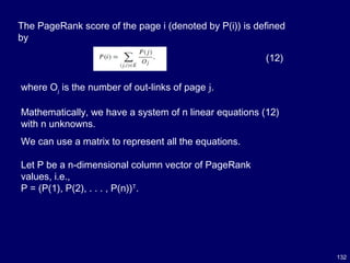
![127
6. PageRank
Overview
PageRank [10] was presented and published by Sergey Brin and Larry
Page at the Seventh International World Wide Web Conference
(WWW7) in April 1998.
It is a search ranking algorithm using hyperlinks on theWeb.
Based on the algorithm, they built the search engine Google, which has
been a huge success.
Now, every search engine has its own hyperlink based ranking method.](https://image.slidesharecdn.com/10candidatelist-160324142046/85/top-10-Data-Mining-Algorithms-127-320.jpg)
![128
PageRank produces a static ranking of Web pages in the sense that a
PageRank value is computed for each page off-line and it does not
depend on search queries.
The algorithm relies on the democratic nature of the Web by using its
vast link structure as an indicator of an individual page’s quality.
In essence, PageRank interprets a hyperlink from page x to page y as a
vote, by page x, for page y.
However, PageRank looks at more than just the sheer number of votes,
or links that a page receives. It also analyzes the page that casts the
vote.
Votes casted by pages that are themselves “important” weigh more
heavily and help to make other pages more “important”. This is exactly
the idea of rank prestige in social networks [86].](https://image.slidesharecdn.com/10candidatelist-160324142046/85/top-10-Data-Mining-Algorithms-128-320.jpg)

![130
The following ideas based on rank prestige [86] are used to derive the
PageRank algorithm:
1. A hyperlink from a page pointing to another page is an implicit
conveyance of authority to the target page. Thus, the more in-
links that a page i receives, the more prestige the page i has.
2. Pages that point to page i also have their own prestige scores. A
page with a higher prestige score pointing to i is more important
than a page with a lower prestige score pointing to i . In other
words, a page is important if it is pointed to by other important
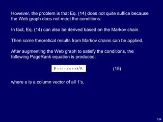
pages.](https://image.slidesharecdn.com/10candidatelist-160324142046/85/top-10-Data-Mining-Algorithms-130-320.jpg)

![133
(13)
Let A be the adjacency matrix of our graph with
We can write the system of n equations
with
P= AT
P. (14)
This is the characteristic equation of the eigensystem, where the
solution to P is an eigenvector with the corresponding eigenvalue
of 1.
Since this is a circular definition, an iterative algorithm is used to
solve it.
It turns out that if some conditions are satisfied, 1 is the largest
eigenvalue and the PageRank vector P is the principal eigenvector.
A well known mathematical technique called power iteration [30]
can be used to find P.](https://image.slidesharecdn.com/10candidatelist-160324142046/85/top-10-Data-Mining-Algorithms-133-320.jpg)
![135
This gives us the PageRank formula for each
page i :
(16)
(17)
which is equivalent to the formula given in the original
PageRank papers [10,61]:
The parameter d is called the damping factor which can be set to a
value between 0 and 1. d = 0.85 is used in [10,52].](https://image.slidesharecdn.com/10candidatelist-160324142046/85/top-10-Data-Mining-Algorithms-135-320.jpg)
![136
The computation of PageRank values of the Web pages can be done
using the power iteration method [30], which produces the principal
eigenvector with the eigenvalue of 1.
The algorithm is simple, and is given in Fig. 1.
One can start with any initial assignments of PageRank values.
The iteration ends when the PageRank values do not change much or
converge.](https://image.slidesharecdn.com/10candidatelist-160324142046/85/top-10-Data-Mining-Algorithms-136-320.jpg)
![137
In Fig. 4 above, the iteration ends after the 1-norm of the residual
vector is less than a pre-specified threshold e.
Since in Web search, we are only interested in the ranking of the
pages, the actual convergence may not be necessary.
Thus, fewer iterations are needed.
In [10], it is reported that on a database of 322 million links the
algorithm converges to an acceptable tolerance in roughly 52
iterations.
The power iteration method for
PageRank](https://image.slidesharecdn.com/10candidatelist-160324142046/85/top-10-Data-Mining-Algorithms-137-320.jpg)
![138
FurtherReferences on PageRank
Since PageRank was presented in [10,61], researchers have
proposed many enhancements to the model, alternative models,
improvements for its computation, adding the temporal dimension
[91], etc. The books by Liu [52] and by Langville and Meyer [49]
contain in-depth analyses of PageRank and several other link-based
algorithms.](https://image.slidesharecdn.com/10candidatelist-160324142046/85/top-10-Data-Mining-Algorithms-138-320.jpg)
![139
7. AdaBoost
Description of the Algorithm
Ensemble learning [20] deals with methods which employ multiple
learners to solve a problem.
The generalization ability of an ensemble is usually significantly
better than that of a single learner, so ensemble methods are very
attractive.
The AdaBoost algorithm [24] proposed by Yoav Freund and Robert
Schapire is one of the most important ensemble methods, since it
has solid theoretical foundation, very accurate prediction, great
simplicity (Schapire
said it needs only “just 10 lines of code”), and wide and successful
applications.](https://image.slidesharecdn.com/10candidatelist-160324142046/85/top-10-Data-Mining-Algorithms-139-320.jpg)

![143
In order to deal with multi-class problems, Freund and Schapire
presented the Ada-Boost.
M1 algorithm [24] which requires that the weak learners are strong
enough even on hard distributions generated during the AdaBoost
process.
Another popular multi-class version of AdaBoost is AdaBoost.MH [69]
which works by decomposing multi-class task to a series of binary
tasks.
AdaBoost algorithms for dealing with regression problems have also
been studied.
Since many variants of AdaBoost have been developed during the past
decade, Boosting has become the most important “family” of ensemble
methods.](https://image.slidesharecdn.com/10candidatelist-160324142046/85/top-10-Data-Mining-Algorithms-143-320.jpg)

![145
In 1988, Kearns and Valiant posed an interesting question, i.e.,
whether a weak learning algorithm that performs just slightly better
than random guess could be “boosted” into an arbitrarily accurate
strong learning algorithm.
In other words, whether two complexity classes, weakly learnable and
strongly learnable problems, are equal.
Schapire [67] found that the answer to the question is “yes”, and the
proof he gave is a construction, which is the first Boosting algorithm.
So, it is evident that AdaBoost was born with theoretical significance.
AdaBoost has given rise to abundant research on theoretical aspects
of ensemble methods, which can be easily found in machine learning
and statistics literature.
It is worth mentioning that for their AdaBoost paper [24], Schapire and
Freund won the Godel Prize, which is one of the most prestigious
awards in theoretical computer science, in the year of 2003.](https://image.slidesharecdn.com/10candidatelist-160324142046/85/top-10-Data-Mining-Algorithms-145-320.jpg)
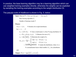
![146
AdaBoost and its variants have been applied to diverse domains with
great success.
For example, Viola and Jones [84] combined AdaBoost with a cascade
process for face detection.
They regarded rectangular features as weak learners, and by using
AdaBoost to weight the weak learners, they got very intuitive features
for face detection.](https://image.slidesharecdn.com/10candidatelist-160324142046/85/top-10-Data-Mining-Algorithms-146-320.jpg)
![148
Further
Research
Many interesting topics worth further studying.
Here we only discuss on one theoretical topic and one applied topic.
Many empirical study show that AdaBoost often does not overfit, i.e.,
the test error of AdaBoost often tends to decrease even after the
training error is zero.
Many researchers have studied this and several theoretical
explanations have been given, e.g. [38].
Schapire et al. [68] presented amargin-based explanation.
They argued that AdaBoost is able to increase the margins even after
the training error is zero, and thus it does not overfit even after a large
number of rounds.](https://image.slidesharecdn.com/10candidatelist-160324142046/85/top-10-Data-Mining-Algorithms-148-320.jpg)
![149
Further
ResearchHowever, Breiman [8] indicated that larger margin does not necessarily
mean better generalization, which seriously challenged the margin-
based explanation.
Recently, Reyzin and Schapire [65] found that Breiman considered
minimum margin instead of average or median margin, which suggests
that the margin-based explanation still has chance to survive.
If this explanation succeeds, a strong connection between AdaBoost
and SVM could be found. It is obvious that this topic is well worth
studying.](https://image.slidesharecdn.com/10candidatelist-160324142046/85/top-10-Data-Mining-Algorithms-149-320.jpg)

![151
However, feature selection methods are usually based on heuristics,
lacking solid theoretical foundation.
Inspired by Viola and Jones’s work [84], we think AdaBoost could be
very useful in feature selection, especially when considering that it has
solid theoretical foundation.
Current research mainly focus on images, yet we think general
AdaBoost-based feature selection techniques are well worth studying.](https://image.slidesharecdn.com/10candidatelist-160324142046/85/top-10-Data-Mining-Algorithms-151-320.jpg)

![153
A more sophisticated approach, k-nearest neighbor (kNN) classification
[23,75], finds a group of k objects in the training set that are closest to
the test object, and bases the assignment of a label on the
predominance of a particular class in this neighborhood.
To classify an unlabeled object, the distance of this object to the labeled
objects is computed, its k-nearest neighbors are identified, and the class
labels of these nearest neighbors are then used to determine the class
label of the object.
There are three key elements of this approach:
a set of labeled objects, e.g., a set of stored records,
a distance or similarity metric to compute distance between
objects,
and the value of k, the number of nearest neighbors.](https://image.slidesharecdn.com/10candidatelist-160324142046/85/top-10-Data-Mining-Algorithms-153-320.jpg)


![159
Some distance measures can also be affected by the high
dimensionality of the data.
In particular, it is well known that the Euclidean distance measure
become less discriminating as the number of attributes increases.
Also, attributes may have to be scaled to prevent distance
measures from being dominated by one of the attributes.
For example, consider a data set where the height of a person
varies from 1.5 to 1.8m, the weight of a person varies from 90 to
300 lb, and the income of a person varies from $10,000 to
$1,000,000.
If a distance measure is used without scaling, the income attribute
will dominate the computation of distance and thus, the assignment
of class labels.
A number of schemes have been developed that try to compute the
weights of each individual attribute based upon a training set [32].](https://image.slidesharecdn.com/10candidatelist-160324142046/85/top-10-Data-Mining-Algorithms-159-320.jpg)
![160
In addition, weights can be assigned to the training objects
themselves.
This can give more weight to highly reliable training objects, while
reducing the impact of unreliable objects.
The PEBLS system by Cost and Salzberg [14] is a well known
example of such an approach.
KNN classifiers are lazy learners, that is, models are not built
explicitly unlike eager learners (e.g., decision trees, SVM, etc.).](https://image.slidesharecdn.com/10candidatelist-160324142046/85/top-10-Data-Mining-Algorithms-160-320.jpg)

![162
Impact
KNN classification is an easy to understand and easy to implement
classification technique.
Despite its simplicity, it can perform well in many situations.
In particular, a well known result by Cover and Hart [15] shows that the
error of the nearest neighbor rule is bounded above by twice the Bayes
error under certain reasonable assumptions.
Also, the error of the general kNN method asymptotically approaches
that of the Bayes error and can be used to approximate it.](https://image.slidesharecdn.com/10candidatelist-160324142046/85/top-10-Data-Mining-Algorithms-162-320.jpg)
![163
KNN is particularly well suited for multi-modal classes as well as
applications in which an object can have many class labels.
For example, for the assignment of functions to genes based on
expression profiles, some researchers found that kNN outperformed
SVM, which is a much more sophisticated classification scheme [48].](https://image.slidesharecdn.com/10candidatelist-160324142046/85/top-10-Data-Mining-Algorithms-163-320.jpg)
![164
Current and Further
Research
Although the basic kNN algorithm and some of its variations, such as
weighted kNN and assigning weights to objects, are relatively well
known, some of the more advanced techniques for kNN are much less
known.
For example, it is typically possible to eliminate many of the stored data
objects, but still retain the classification accuracy of the kNN classifier.
This is known as ‘condensing’ and can greatly speed up the
classification of new objects [35].](https://image.slidesharecdn.com/10candidatelist-160324142046/85/top-10-Data-Mining-Algorithms-164-320.jpg)
![165
In addition, data objects can be removed to improve classification
accuracy, a process known as “editing” [88].
There has also been a considerable amount of work on the application
of proximity graphs (nearest neighbor graphs, minimum spanning trees,
relative neighborhood graphs, Delaunay triangulations, and Gabriel
graphs) to the kNN problem.
Recent papers by Toussaint [79,80], which emphasize a proximity graph
viewpoint, provide an overview of work addressing these three areas
and indicate some remaining open problems.
Other important resources include the collection of papers by Dasarathy
[16] and the book by Devroye et al. [18].
Finally, a fuzzy approach to kNN can be found in the work of Bezdek [4].](https://image.slidesharecdn.com/10candidatelist-160324142046/85/top-10-Data-Mining-Algorithms-165-320.jpg)

![167
The naive Bayes method is important for several reasons.
It is very easy to construct, not needing any complicated iterative
parameter estimation schemes.
The method may be readily applied to huge data sets.
It is easy to interpret, so users unskilled in classifier technology can
understand why it is making the classification it makes.
And finally, it often does surprisingly well: it may not be the best possible
classifier in any particular application, but it can usually be relied on to
be robust and to do quite well.
General discussion of the naive Bayes method and its merits are given in
[22,33].](https://image.slidesharecdn.com/10candidatelist-160324142046/85/top-10-Data-Mining-Algorithms-167-320.jpg)


![181
Concluding Remarks on Naïve Bayes
The naive Bayes model is tremendously appealing because of its
simplicity, elegance, and robustness.
It is one of the oldest formal classification algorithms, and yet even in
its simplest form it is often surprisingly effective.
It is widely used in areas such as text classification and spam
filtering.
A large number of modifications have been introduced, by the
statistical,
data mining, machine learning, and pattern recognition communities,
in an attempt to make it more flexible, but one has to recognize that
such modifications are necessarily complications, which detract from
its basic simplicity.
Some such modifications are described in [27,66].](https://image.slidesharecdn.com/10candidatelist-160324142046/85/top-10-Data-Mining-Algorithms-181-320.jpg)


![188
The CART authors favor the Gini criterion over information gain
because the Gini can be readily extended to include symmetrized
costs (see below) and is computed more rapidly than information gain.
(Later versions of CART have added information gain as an optional
splitting rule.)
They introduce the modified twoing rule, which is based on a direct
comparison of the target attribute distribution in two child nodes:
(29)
where k indexes the target classes, pL() and pR() are the probability
distributions of the target in the left and right child nodes respectively,
and the power term u embeds a user-trollable penalty on splits
generating unequal-sized child nodes.
This splitter is a modified version of Messenger and Mandell [58].](https://image.slidesharecdn.com/10candidatelist-160324142046/85/top-10-Data-Mining-Algorithms-188-320.jpg)


![192
Missing Value Handling
Missing values appear frequently in real world, and especially
business-related databases, and the need to deal with them is a
vexing challenge for all modelers.
One of the major contributions of CART was to include a fully
automated and highly effective mechanism for handling missing
values.
Decision trees require a missing value-handling mechanism at three
levels:
(a) during splitter evaluation,
(b) when moving the training data through a node, and
(c) when moving test data through a node for final class
assignment. (See [63] for a clear discussion of these
points.)](https://image.slidesharecdn.com/10candidatelist-160324142046/85/top-10-Data-Mining-Algorithms-192-320.jpg)
![194
Friedman [25] suggested moving instances with missing splitter
attributes into both left and right child nodes and making a final class
assignment by pooling all nodes in which an instance appears.
Quinlan [63] opted for a weighted variant of Friedman’s approach in
his study of alternative missing value-handling methods.
Our own assessments of the effectiveness of CART surrogate
performance in the presence of missing data are largely favorable,
while Quinlan remains
agnostic on the basis of the approximate surrogates he implements
for test purposes [63].
Friedman et al. [26] noted that 50% of the CART code was devoted
to missing value handling; it is thus unlikely that Quinlan’s
experimental version properly replicated the entire CART surrogate
mechanism.](https://image.slidesharecdn.com/10candidatelist-160324142046/85/top-10-Data-Mining-Algorithms-194-320.jpg)

![198
Dynamic Feature Construction
Friedman [25] discussed the automatic construction of new features
within each node and, for the binary target, recommends adding the
single feature
x ∗ w,
where x is the original attribute vector and w is a scaled difference of
means vector across the two classes (the direction of the Fisher linear
discriminant).
This is similar to running a logistic regression on all available
attributes in the node and using the estimated logit as a predictor.
In the CART monograph, the authors discuss the automatic
construction of linear combinations that include feature selection; this
capability has been available from the first release of the CART
software.
BFOS also present a method for constructing Boolean combinations](https://image.slidesharecdn.com/10candidatelist-160324142046/85/top-10-Data-Mining-Algorithms-198-320.jpg)
![199
Cost-Sensitive Learning
Costs are central to statistical decision theory but cost-sensitive
learning received onlymodest attention before Domingos [21].
Since then, several conferences have been devoted exclusively to
this topic and a large number of research papers have appeared in
the subsequent
scientific literature.
It is therefore useful to note that the CART monograph introduced
two
strategies for cost-sensitive learning and the entire mathematical
machinery describing CART is cast in terms of the costs of
misclassification.](https://image.slidesharecdn.com/10candidatelist-160324142046/85/top-10-Data-Mining-Algorithms-199-320.jpg)
![201
The first and most straightforward method for handling costs makes
use of weighting: instances belonging to classes that are costly to
misclassify are weighted upwards, with a common weight applying
to all instances of a given class, a method recently rediscovered by
Ting [78].
As implemented in CART, the weighting is accomplished
transparently so that
all node counts are reported in their raw unweighted form.
For multi-class problems BFOS suggested that the entries in the
misclassification cost matrix be summed across each row to obtain
relative class weights that approximately reflect costs.
This technique ignores the detail within the matrix but has now been
widely adopted due to its simplicity.](https://image.slidesharecdn.com/10candidatelist-160324142046/85/top-10-Data-Mining-Algorithms-201-320.jpg)


![208
The CART monograph offers a some what more complex method to
adjust the terminal node estimates that has rarely been discussed in
the literature.
Dubbed the “Breiman adjustment”, it adjusts the estimated
misclassification rate r*(t) of any terminal node upwards by
r ∗(t) = r (t) + e/(q(t) + S) (32)
where r (t) is the train sample estimate within the node, q(t) is the
fraction of the training sample in the node and S and e are
parameters that are solved for as a function of the difference between
the train and test error rates for a given tree.
In contrast to the LaPlace method, the Breiman adjustment does not
depend on the raw predicted probability in the node and the
adjustment can be very small if the test data show that the tree is not
overfit.
Bloch et al. [5] reported very good performance for the Breiman
adjustment in a series of empirical experiments.](https://image.slidesharecdn.com/10candidatelist-160324142046/85/top-10-Data-Mining-Algorithms-208-320.jpg)


![213
Leo Breiman earned his BA in Physics at the California Institute of
Technology, his PhD in Mathematics at UC Berkeley, and made
notable contributions to pure probability theory (Breiman, 1968) [7]
while a Professor at UCLA.
In 1967 he left academia for 13 years to work as an industrial
consultant; during this time he encountered the military data
analysis problems that inspired his contributions to CART.
An interview with Leo Breiman discussing his career and personal
life appears in [60].](https://image.slidesharecdn.com/10candidatelist-160324142046/85/top-10-Data-Mining-Algorithms-213-320.jpg)
![216
11. Concluding Remarks
Data mining is a broad area that integrates techniques from several
fields including machine learning, statistics, pattern recognition,
artificial intelligence, and database systems, for the analysis of large
volumes of data.
There have been a large number of data mining algorithms rooted
in these fields to perform different data analysis tasks.
The 10 algorithms identified by the IEEE International Conference
on Data Mining (ICDM) and presented in this article are among the
most influential algorithms for classification [47,51,77], clustering
[11,31,40,44–46], statistical learning [28,76,92], association
analysis [2,6,13,50,54,74],
and link mining.](https://image.slidesharecdn.com/10candidatelist-160324142046/85/top-10-Data-Mining-Algorithms-216-320.jpg)


The document discusses the top ten recent innovations, algorithms, and challenging tasks in data mining, highlighting inventions that have significantly changed daily life, like GPS technology and social networking. It further outlines the ten most pressing issues in data mining research, including the need for a unifying theory, handling high-dimensional data, and ensuring privacy and security in data mining processes. The document also lists influential algorithms in data mining, compiled through expert nominations and community voting.