Tom&md notes module 03

Module 3: Types of loads and stresses, theories of failure, factor of safety, selection of
allowable Stress. Stress concentration. Elementary fatigue and creep aspects. Design of
Cotter joints, knuckle joint and, Design of flange couplings.
Stress & Strain
When a force is applied to a structural member, that member will develop both stress and
strain as a result of the force. Stress is the force carried by the member per unit area, and
typical units are lbf/in2
(psi) for US Customary units and N/m2
(Pa) for SI units:
σ =
𝐹
𝐴
where F is the applied force and A is the cross-sectional area over which the force acts. The
applied force will cause the structural member to deform by some length, in proportion to
its stiffness. Strain is the ratio of the deformation to the original length of the part:
ɛ =
𝐿 − L0
L0
where L is the deformed length, L0 is the original undeformed length, and δ is the
deformation (the difference between the two).
There are different types of loading which result in different types of stress
Loading Type Stress Type Illustration
Axial Force
• Axial Stress
(general case)
• Tensile Stress
(if force is tensile)
• Compressive Stress
(if force is
compressive)
Shear Force Transverse Shear Stress
Bending Moment Bending Stress
Torsion Torsional Stress
Theories of Failure

When a machine element is subjected to a system of complex stress system, it is important to
predict the mode of failure so that the design methodology may be based on a particular
failure criterion. Theories of failure are essentially a set of failure criteria developed for the
ease of design. In machine design an element is said to have failed if it ceases to perform its
function.
There are basically two types of mechanical failure:
1. Yielding- This is due to excessive inelastic deformation rendering the machine part
unsuitable to perform its function. This mostly occurs in ductile materials.
2. Fracture- in this case the component tears apart in two or more parts. This mostly occurs
in brittle materials.
Failure: In order to design the cotton joint and find out the dimensions, failure, in different
parts and different cross-sections are considered.
There are many instances when a ductile material may fail by fracture. This may occur if a
material is subjected to
(a) Cyclic loading
(b) Long term static loading at elevated temperature
(c) Impact loading
(d) Work hardening
(e) Severe quenching
Factor of safety (f.o.s): The ratio of ultimate to allowable load or stress is known as factor of
safety i.e. The factor of safety can be defined as the ratio of the material strength or failure
stress to the allowable or working stress.
The factor of safety must be always greater than unity. It is easier to refer to the ratio of
stresses since this applies to material properties.
f.o.s = failure stress / working or allowable stress
Ductile and Brittle Materials A ductile material deforms significantly before fracturing.
Ductility is measured by % elongation at the fracture point. Materials with 5% or more
elongation are considered ductile The limiting strength of ductile materials is the stress at
yield point.

A brittle material yields very little before fracturing; the yield strength is approximately the
same as the ultimate strength in tension. The limiting strength of brittle materials is the
ultimate stress
Static Failure Theories Predicting failure in members subjected to uni-axial stress is both
simple and straight-forward. But, predicating the failure stresses for members subjected to bi-
axial or tri-axial stresses is much more complicated.A large numbers of different theories
have been formulated. The principal theories of failure for a member subjected to biaxial
stress are as follows:
Maximum Principal/Normal Stress Theory (Rankine’s Theory)
Maximum Shear Stress Theory (Guest’s Theory)
Maximum Principal /Normal Strain Theory (Saint’s Theory)
Maximum Strain Energy Theory (Haigh’s Theory)
Maximum Distortion Energy Theory (Hencky & Von Mises Theory)
Maximum Principal Stress Theory (Rankine Theory):
If one of the principal stresses σ1 (maximum principal stress), σ2 (minimum principal stress)
or σ3 exceeds the yield stress, yielding would occur.
In a two dimensional loading situation for a ductile material where tensile and compressive
yield stress are nearly of same magnitude:
Yielding occurs when the state of stress is at the boundary of the rectangle.
At a point a, the stresses are still within the elastic limit but at b, σ1 reaches σy although σ2 is
still less than σy.
Yielding will then begin at point b
Maximum Principal Strain Theory (St. Venant’s theory):

Yielding will occur when the maximum principal strain just exceeds the strain at the tensile
yield point in either simple tension or compression. If ε1 and ε2 are maximum and minimum
principal strains corresponding to σ1 and σ2, in the limiting case
It implies
Boundary of a yield surface in Maximum Strain Energy Theory is given below
Maximum Shear Stress Theory (Tresca Theory):
Yielding would occur when the maximum shear stress just exceeds the shear stress at the
tensile yield point. At the tensile yield point σ2= σ3 = 0 and thus maximum shear stress is
σy/2.

This gives us six conditions for a three-dimensional stress situation:
Yield surface corresponding to maximum shear stress theory in biaxial stress situation is
given below :
Maximum strain energy theory ( Beltrami’s theory):
Failure would occur when the total strain energy absorbed at a point per unit volume exceeds
the strain energy absorbed per unit volume at the tensile yield point. This may be given
Substituting, ε1, ε2 , ε3 and εy in terms of stresses we have

Above equation results in Elliptical yield surface which can be viewed as:
Distortion energy theory (Von Mises yield criterion):
Yielding would occur when total distortion energy absorbed per unit volume due to applied
loads exceeds the distortion energy absorbed per unit volume at the tensile yield point. Total
strain energy ET and strain energy for volume change EV can be given as:
Substituting strains in terms of stresses the distortion energy can be given as
At the tensile yield point, σ1 = σy , σ2 = σ3 = 0 which gives,

In a 2-D situation if σ3 = 0, so the equation reduces to
This is an equation of ellipse and yield equation is an ellipse. This theory is widely accepted
for ductile materials

Stress Concentration
The basic stress equations for tension, compression, bending, and torsion are based on a
number of assumptions. One of the assumptions is that there are no geometric irregularities
or abrupt change in the cross-section of the member. But these irregularities and changes in
the cross-section of members are unavoidable. There will be holes, oil grooves, notches,
keyways, splines, screw threads etc.
Figure Stress Concentration
Any of the discontinuities in a machine part alters the distribution of stress in its vicinity and
localized stress much higher than those calculated with the elementary stress equations are
observed. This localization of high stresses due to geometrical irregularities or abrupt
changes of the cross-section is called ‘stress concentration’ and the discontinuities are called
stress raisers. Stress concentrations can also arise from some irregularity. Stress distribution
in a plate with a small circular hole, subjected to tensile load, is shown in figure. In addition
to the abrupt changes in the cross-section, other causes of stress concentration can be
variation in material properties e.g. internal cracks, flaws, air holes, foreign inclusions etc.
and surface irregularities like scratches or stamp marks.
To consider the effect of stress concentration, stress concentration factor is used, which is the
ratio of maximum stress to nominal stress.
Stress concentration factor for normal stress, Stress concentration factor for shear stress,
Where, σmax , ɽmax= localized stresses near the discontinuities
σ0, ɽ0 = Nominal stresses as determined by elementary equations for minimum cross-section
For the plate shown in figure, if ‘w’ and ‘t’ are width and thickness of the plate, ‘d’ is
diameter of the hole and ‘P’ is the applied load, nominal tensile stress is given by,

Value of stress-concentration factor depends on the geometry of the part only and is
independent of the material used. For this reason, it is called theoretical or geometric stress-
concentration factor. Stress-concentration factors for different geometric shapes are found by
using experimental techniques like photo-elasticity, grid methods, brittle-coating methods,
and electrical strain-gauge methods. The finite-element method has also been used.
Theoretical stress concentration factors for different configurations are available in
handbooks, few of which are shown in figures below [charts for stress concentration factors
are to be provided here].
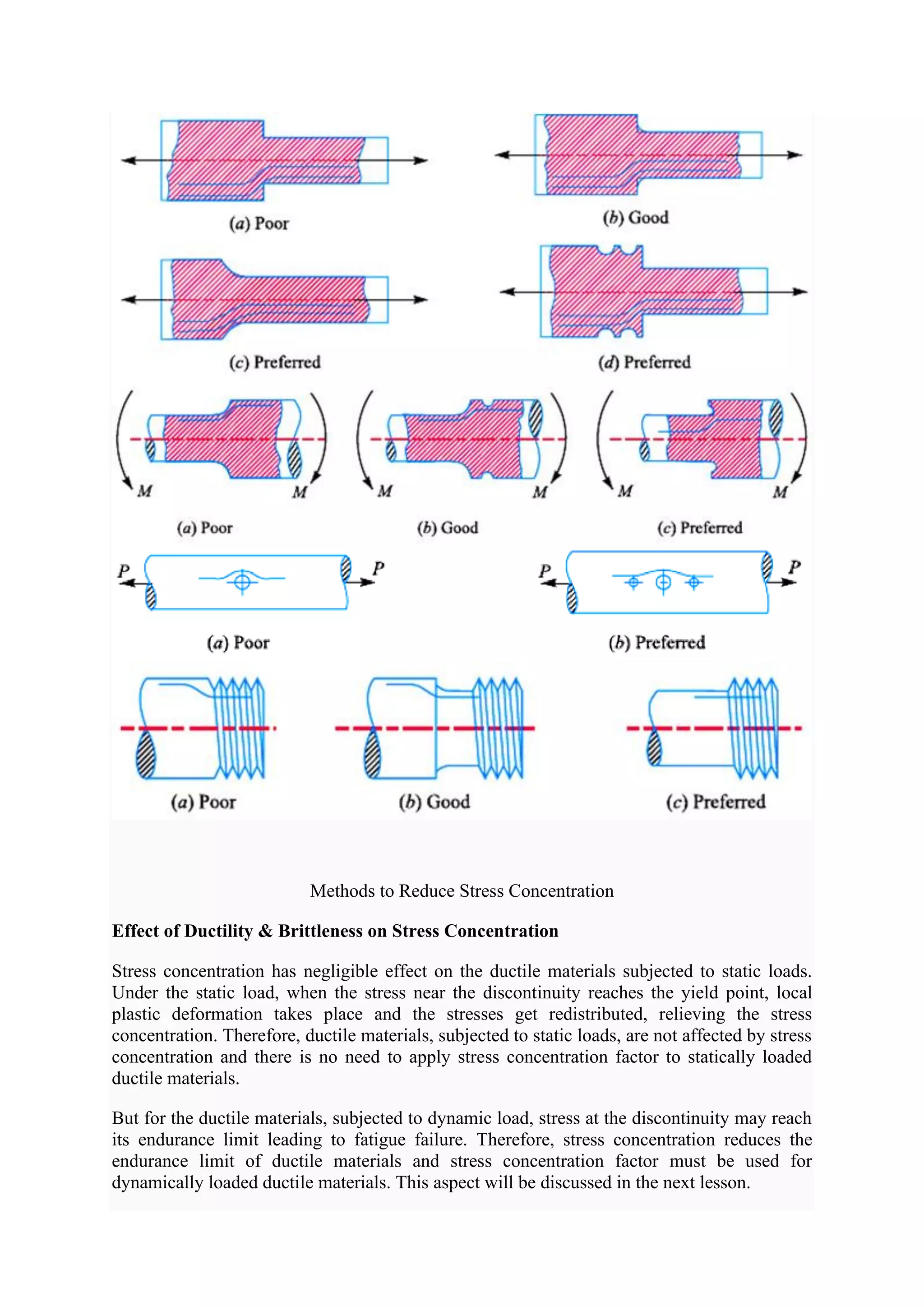
Methods to Reduce Stress Concentration
Effect of stress concentration cannot be completely eliminated but its effect can be reduced
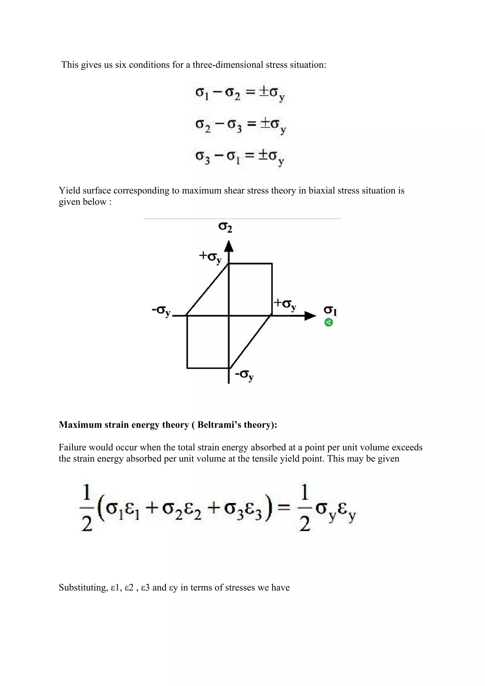
by slightly altering the geometry of the components. Flow analogy is helpful in understanding
how a particular discontinuity affects the stress distribution around it and how its effect can
be reduced.
Figure 5.2 shows the stress distribution in an axially loaded plate which is similar to the
velocity distribution in fluid flow in a channel. For a channel having uniform cross-
section, velocities are uniform and streamlines are equally spaced. If the cross-section of the
channel is suddenly reduced, velocity increases to maintain same flow and the stream
lines become narrower. Similarly, with reduction in cross-section, to transmit same force, the
stress lines come closer. Location where the cross-section changes, stress lines bend as the
stream lines do. Sudden change in the cross-section leads to very sharp bending of stress lines
which results in stress concentration. Therefore by avoiding severe bending of the stress
lines, effect of stress concentration can be reduced. Figure Below shows certain methods to
reduce stress concentration.

Methods to Reduce Stress Concentration
Effect of Ductility & Brittleness on Stress Concentration
Stress concentration has negligible effect on the ductile materials subjected to static loads.
Under the static load, when the stress near the discontinuity reaches the yield point, local
plastic deformation takes place and the stresses get redistributed, relieving the stress
concentration. Therefore, ductile materials, subjected to static loads, are not affected by stress
concentration and there is no need to apply stress concentration factor to statically loaded
ductile materials.
But for the ductile materials, subjected to dynamic load, stress at the discontinuity may reach
its endurance limit leading to fatigue failure. Therefore, stress concentration reduces the
endurance limit of ductile materials and stress concentration factor must be used for
dynamically loaded ductile materials. This aspect will be discussed in the next lesson.

Stress concentration has more severe effect on the brittle materials due to their inability to
plastically deform. As there is no local yielding, stresses don’t get redistributed and local
stress due to discontinuity increases highly. Therefore, stress concentration factor must be
used for components made of brittle materials subjected to static or dynamic loads.
Creep
When components are subjected to constant loads continuously for a longer period, they may
undergo progressive elastic deformation over time. This time-dependent strain is called creep.
Creep can be defined as slow and progressive deformation of material with time under
constant stress. Creep deformation is a function of stress and temperature. It generally occurs
at absolute temperatures above half the melting point of the material and is even present at
room temperature for materials like aluminium, copper and some plastics. Creep increases
with the increase in temperature, and therefore becomes very important for components
operating at higher temperatures like those of furnaces, steam & gas turbines, internal
combustion engines, nuclear reactors, rocket engines etc. The stress can be tensile,
compressive, bending or shear.
Components operating at higher temperatures must be designed in such a way that
deformation due to creep remains within the allowable limit and also creep deformation
doesn’t lead to rupture so that the product performs satisfactorily over time. Creep strength
and creep rupture strength are the two important properties of the material related to creep
design.
Creep Strength is the maximum stress that the material can withstand for a specified length of
time without excessive deformation. Creep Rupture Strength is the maximum stress that the
material can withstand for a specified length of time without rupture.
Figure shows a typical strain vs time plot known as creep curve. To obtain creep curve,
specimen is loaded with a constant force and variation of its length is observed at a constant
elevated temperature. Units of strain are mm/mm and time is measured in hours. When the
load is applied in the beginning of the test, some instantaneous elastic deformation or initial
strain occurs. Then with the passage of time, creep strain occurs. Creep curve is divided into
three stages, primary, secondary and tertiary creep, after which the rupture takes place. In the
start, strain increases rapidly, known as primary. In the secondary creep, strain increases
slowly at a constant rate. Again during the tertiary stage, strain rate increases and necking of
the specimen takes place followed by rupture. The creep test is repeated over a range of
temperatures to obtain a number of creep curves that are useful for design.
Fatigue Curve (S-N Curve) & Endurance Limit

Fatigue properties of the materials are obtained with the help of standard rotating beam test,
in which a highly polished circular section specimen, shown in figure 6.2, is subjected to
cyclic loads. Specimen subjected to constant bending moment is rotated at a very high speed
due to which fibers of the specimen (except those on neutral axis) undergo repeated stress
reversals (maximum tensile stress to maximum compressive stress). Stress-time plot is shown
in figure 6.3. Test is repeated for a number of similar specimens, subjecting them to different
values of stress and number of stress reversals that the specimen survives before fracture are
counted. First test is performed by subjecting the specimen to stress, below ultimate tensile
strength and subsequent tests are performed at decreased levels of stress.
Completely Reversed Stress
Stress-time Plot
Results of the tests are plotted between stress (S) and number of cycles (N), generally on a
log-log scale. S-N Curve is shown in figure
S-N Curve

The ordinate of the S-N curve is called Fatigue Strength (Sf), which can be defined as the
maximum stress that the material can withstand for a specified number of stress reversals. For
ferrous metals and their alloys, S-N curve becomes horizontal after 106
to 107
cycles, which
means that the material can survive infinite number of stress reversals, if the induced stress is
below this level. Stress corresponding to this horizontal line is called endurance limit or
fatigue limit.
Fatigue or Endurance Limit (S'e) can be defined as maximum amplitude of completely
reversed stress that the standard specimen can sustain for an unlimited number of cycles
without fatigue failure. Study of fatigue in which failure takes place before 1000 cycles is
called Low Cycle Fatigue. High Cycle Fatigue is concerned with failure corresponding to
stress cycles greater than 1000 cycles.
In the absence of experimental fatigue data, following relations are sometimes used:
For Steel, S'e = 0.5 Sut
For Cast Iron, S'e = 0.4 Sut

DESIGN OF COTTER JOINT
Cotter joint is used to connect two rods subjected to axial tensile or compressive loads. It is
not suitable to connect rotating shafts which transmit torque. Axes of the rods to be joined
should be collinear. There is no relative angular movement between rods. Cotter joint is
widely used to connect the piston rod and crosshead of a steam engine, as a joint between the
piston rod and the tailor pump rod, foundation bolt etc.
Cotter Joint has mainly three components – spigot, socket and cotter as shown in Figure.
Spigot is formed on one of the rods and socket is formed on the other. The socket and the
spigot are provided with a narrow rectangular slot. The cotter is tightly fitted in this slot.
Spigot fits inside the socket and the cotter is passed through both the socket and the spigot. A
cotter is a wedge shaped piece made of a steel plate. It has uniform thickness and the width
dimension is given a slight taper. Taper is usually 1 in 24 and provides mainly two benefits: i)
cotter becomes tight in the slot due to wedge action. This ensures tightness of the joint in
operating conditions and prevents loosening of the parts. ii) Due to its taper shape, it is easy
to remove the cotter and dismantle the joint.
The construction of cotter joint, used to connect two rods subjected to tensile force P is
shown in the figure. When the cotter is inserted into the slot, the central portion of cotter
comes in contact with spigot and the spigot gets pushed into the socket till the collar of the
spigot comes in contact with the collar of socket. As shown in the figure, finally the cotter is
in contact with the spigot on one side having some clearance with the socket slot and is in
contact with the socket on the other side having some clearance with the spigot slot.
Clearance provided is generally 1.5 to 3 mm. Cotter gets locked because of the frictional
force of the contacting surfaces.
Advantages of Cotter Joint:
- Simple to design and manufacture.
- Simple to assemble and dismantle.
- Very high tightening force due to wedge action, which prevents loosening of parts in
service.

Notations Used :
d = diameter of each rod (mm)
d1 = outside diameter of socket (mm)
d2 = diameter of spigot or inside diameter of socket (mm)
d3 = diameter of spigot-collar (mm)
d4 = diameter of socket-collar (mm)
a = distance from end of slot to the end of spigot on rod-B (mm)
b = mean width of cotter (mm)
c = axial distance from slot to end of socket collar (mm)
t = thickness of cotter (mm)
t1 = thickness of spigot collar (mm)
l = length of cotter (mm)
Assumption for stress analysis of Cotter Joint :
- The rods are subjected to axial tensile force.
- The effect of stress concentration due to holes is neglected
- The force is uniformly distributed in different parts.
Free body diagram of forces acting on three components of the cotter joint (socket, cotter and
spigot) are shown in Figure

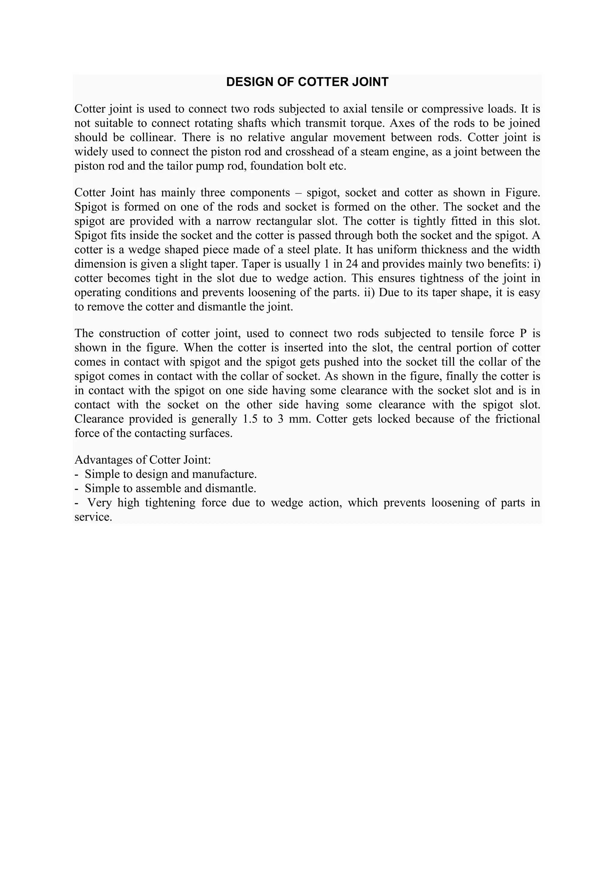
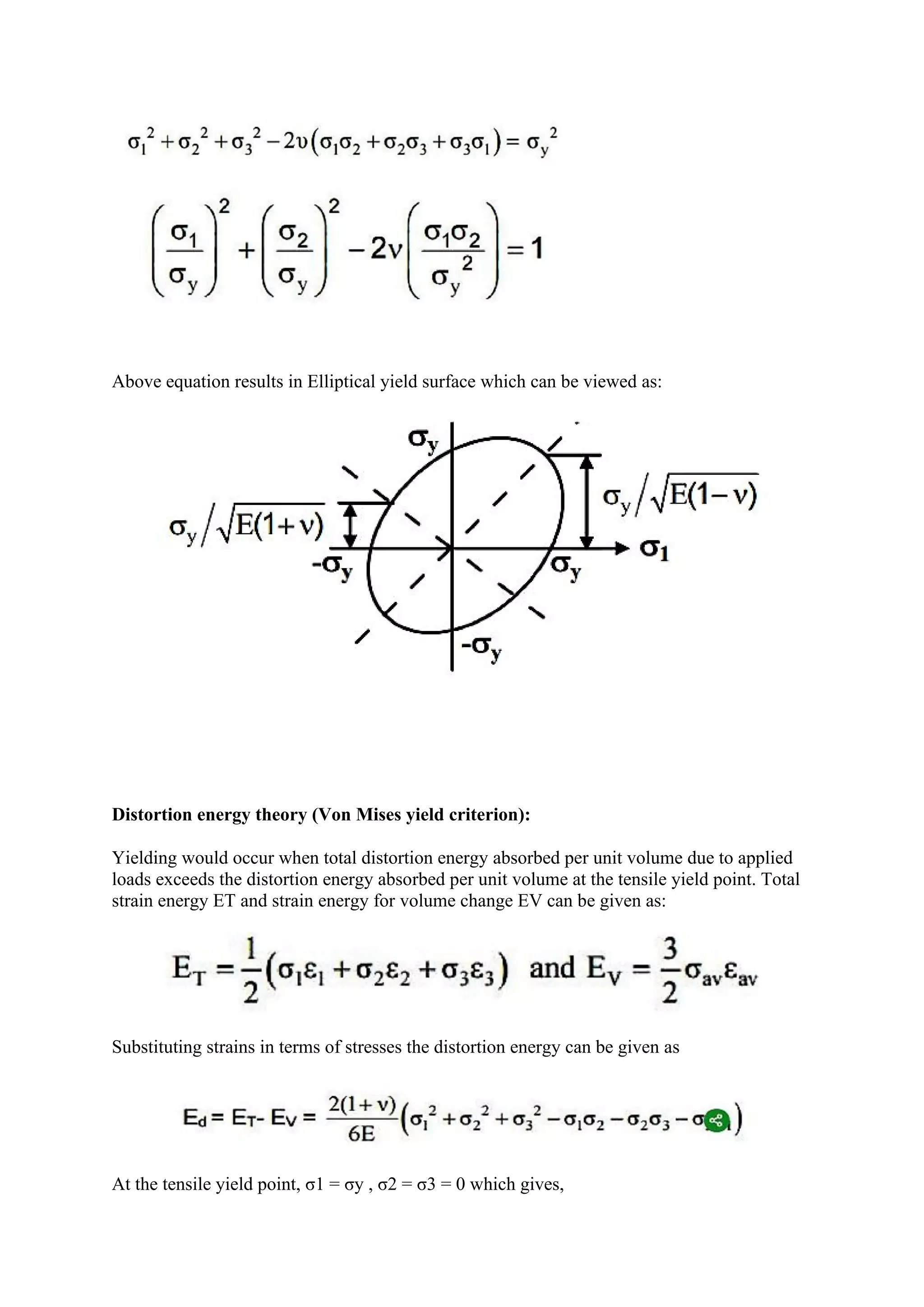
In order to find out various dimensions of the parts of a cotter joint, failures in different parts
and at different x-sections are considered. The stresses developed in the components should
be less than the corresponding permissible values of stress. So, for each type of failure, one
strength equation is written and these strength equations are then used to find various
dimensions of the cotter joint. Some empirical relations are also used to find the dimensions.
Possible Modes of Failure of Cotter Joint
1-Tensile Failure of Rods :
Each rod is subjected to a tensile force P.
Tensile stress in the rods =
where [σ] = allowable tensile stress for the material selected.
2-Tensile Failure of Spigot :
Area of the weakest section of spigot resisting tensile failure =
𝛱
4
𝑑2
2
− 𝑑2𝑡
Tensile Stress in the Spigot =
Tensile Failure of Spigot

3-Tensile Failure of Socket :
Area of the weakest section of socket resisting tensile failure =
𝛱
4
(𝑑1
2
− 𝑑2
2
) − (𝑑1 − 𝑑2)𝑡
Tensile Stress in the Socket =
Tensile Failure of Socket
4-Shear Failure of Spigot End :
The spigot end is subjected to double shear.
Total area that resists the shear failure = 2ad2
Shear Stress in the socket =
where ɽ = allowable shear stress for the material selected. Shear Failure of Spigot End
5-Shear Failure of Socket End :
The socket end is subjected to double shear.
Total area that resists the shear failure =2(d4-d2) c
Shear Failure of Socket End

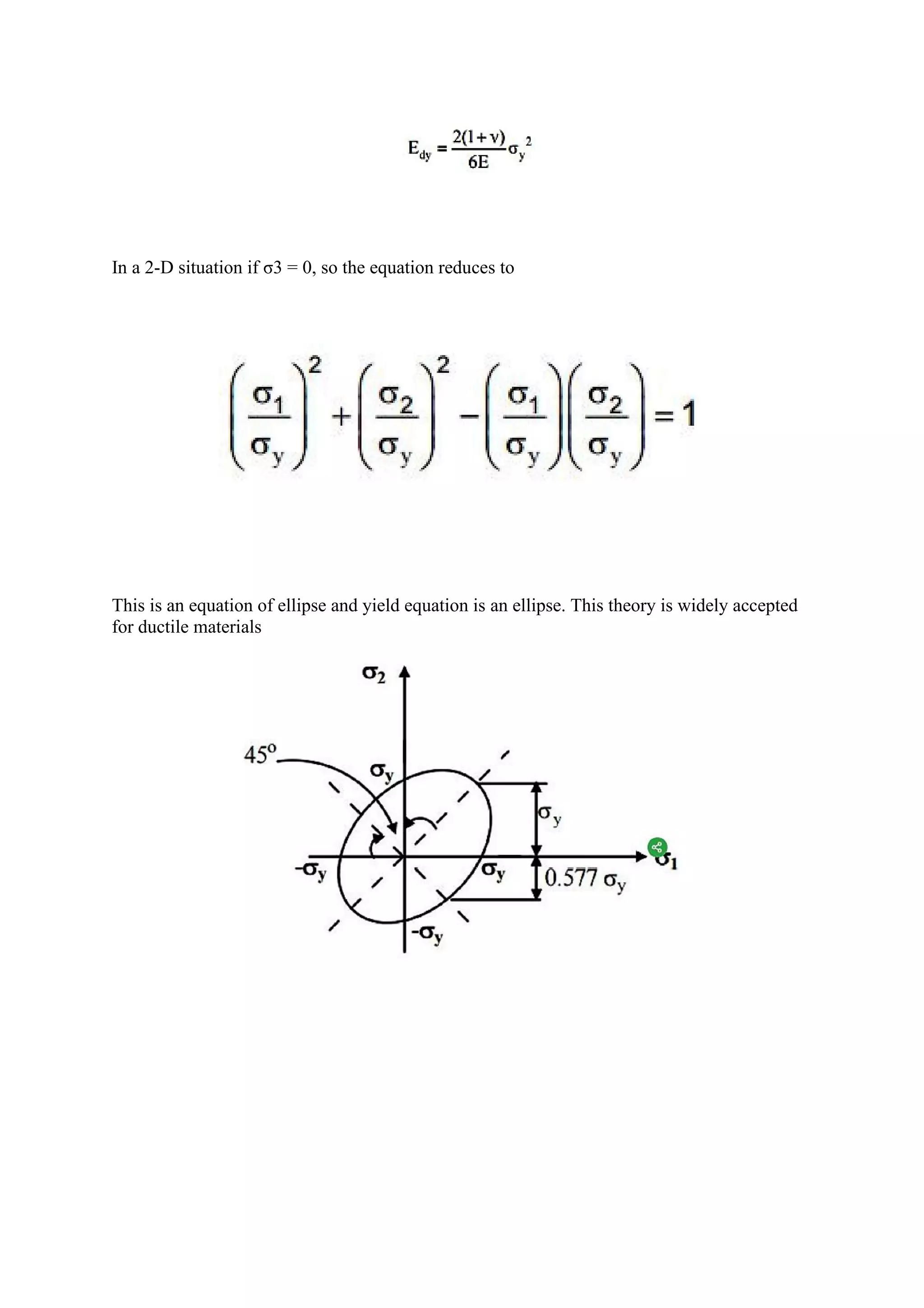
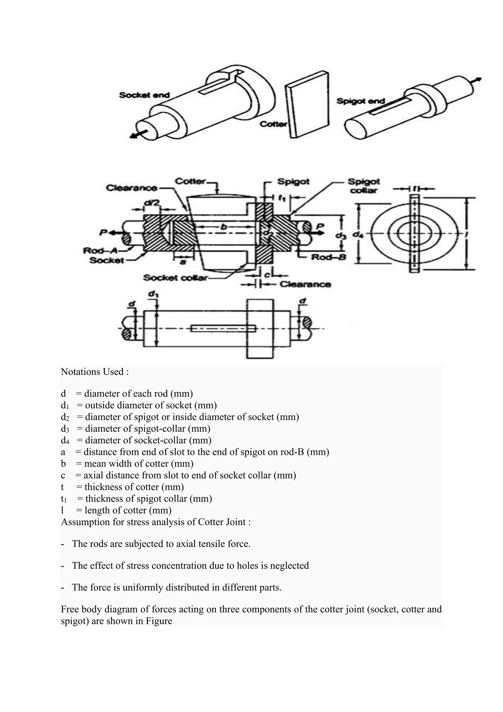
6. Crushing Failure of Spigot End :
Area under crushing = td2
Crushing Stress =
where [σc] = allowable compressive stress for the material selected. Crushing Failure of Spigot End
7. Crushing Failure of Socket End :
Area under crushing = (d4 - d2)t
Crushing Stress,
Crushing Failure of Socket
8. Shear Failure of Spigot Collar :
Area of spigot collar that resists the shear failure = 𝚷 d2 t1
Area of spigot collar that resists the shear failure
9. Crushing Failure of Spigot Collar :
Area of spigot collar under crushing ==
𝜫
𝟒
(𝒅𝟑
𝟐
− 𝒅𝟐
𝟐
)
Crushing Stress =
Area of spigot collar under crushing
10. Shear Failure of Cotter :
The cotter is subjected to double shear.
Total area of cotter that resists the shear failure = 2bt
Shear Stress in the pin =
Shear Failure of Cotter

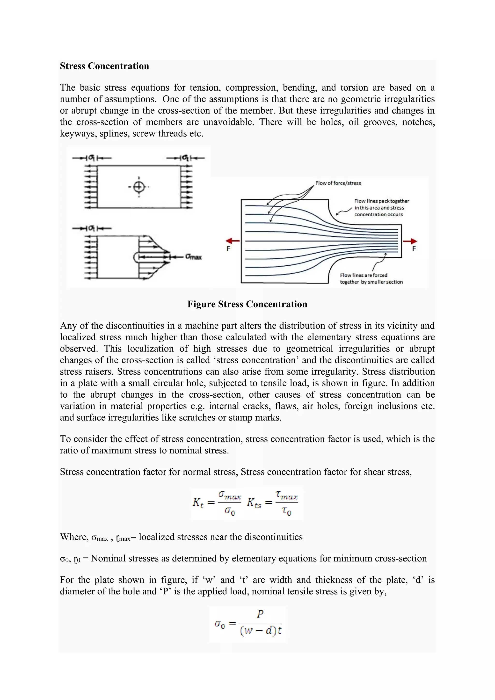
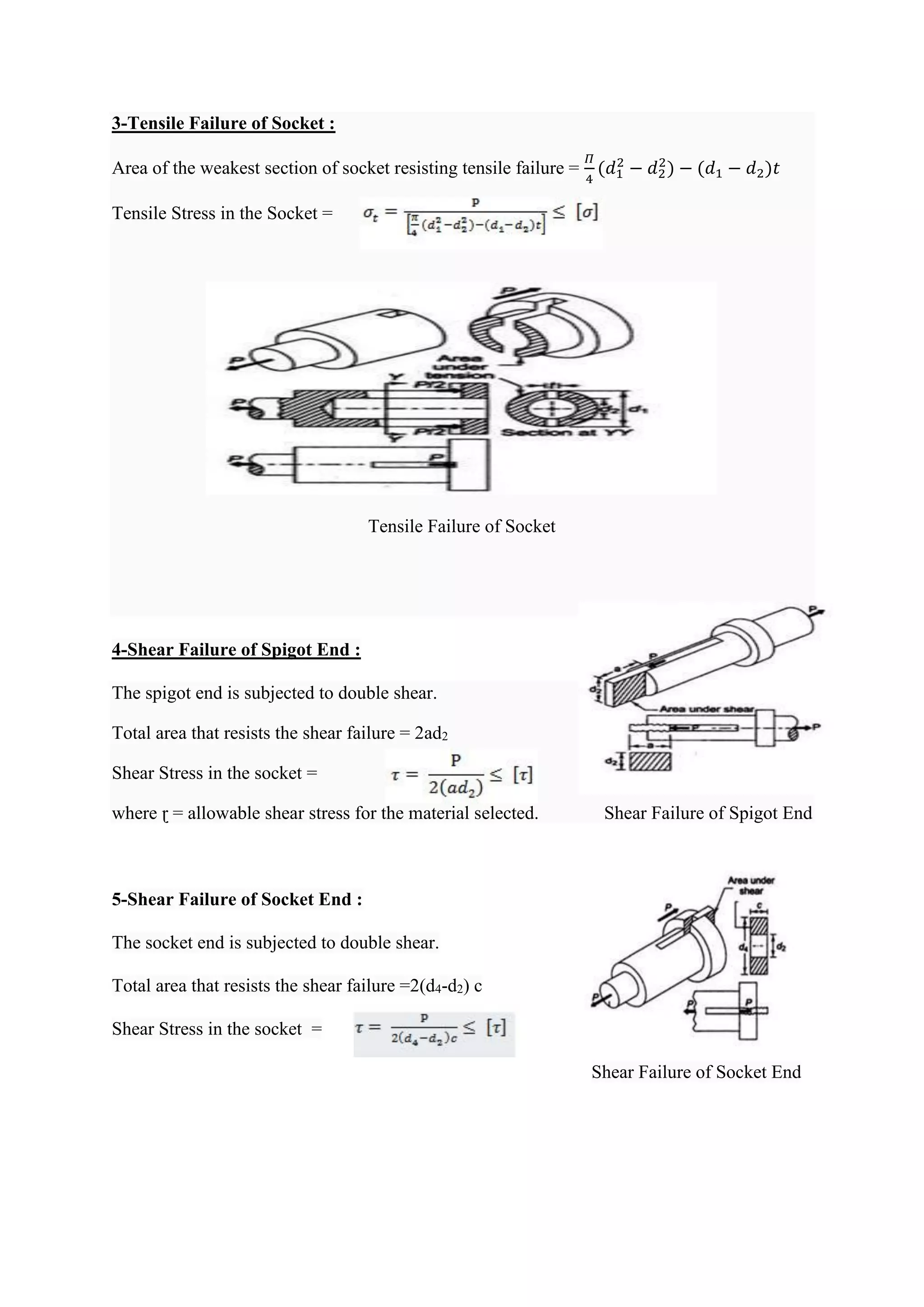
Design Procedure for Cotter Joint
Procedure to determine various dimensions of cotter joint is as follows:
i) Calculate the Diameter of each rod
ii) Calculate thickness of cotter using empirical relation [t = 0.31d]
iii) Calculate diameter of the spigot on the basis of tensile stress=
iv) Calculate outside diameter of the socket on the basis of tensile stress =
v) Diameter of spigot collar, d3 and diameter of socket collar, d4 are determined using
empirical relations d3 = 1.5 d and d4 = 2.4 d
vi) Dimensions a and c are also determined using empirical relations a = c = 0.75 d.
vii) Calculate width of cotter by shear consideration =
viii) Check the crushing and shear stresses in the spigot end.
And
ix) Check the crushing and shear stresses in the socket end
and
x) Calculate thickness t1 of spigot collar by the following empirical relationship = [t1 = 0.45d]
xi) Check the crushing and shear stresses in the spigot collar
and
Question 01 Design and draw a cotter joint to support a load varying from 30 kN in
compression to 30 kN in tension. The material used is carbon steel for which the following
allowable stresses may be used. The load is applied statically.
Tensile stress = compressive stress = 50 MPa ; shear stress = 35 MPa and crushing stress =
90 MPa
Question 02 Design a cotter joint to connect two mild steel rods for a pull of 30 kN. The
maximum permissible stresses are 55 MPa in tension ; 40 MPa in shear and 70 MPa in
crushing. Draw a neat sketch of the joint designed.

Knuckle Joint
Knuckle joint is used to connect two rods subjected to axial tensile loads. It may also be used
to support the compressive load if the joint is guided. It is not suitable to connect rotating
shafts which transmit torque. Axes of the shafts to be joined should lie in the same plane and
may coincide or intersect. Its construction permits limited relative angular movement
between rods, about the axis of the pin. Knuckle joint is widely used to connect valve rod and
eccentric rod, in the link of a cycle chain, levers, tie rod joint for roof truss and many other
links.
Knuckle Joint has mainly three components – eye, fork and pin as shown in Figure 8.1. Eye is
formed on one of the rods and fork is formed on the other. Eye fits inside the fork and the pin
is passed through both the fork and the eye. This pin is secured in its place by means of a
split-pin. The ends of the rods are made octagonal to some distance for better grip and are
made square for some portion before it is forged to make the eye and fork shapes.
Advantages of Knuckle Joint are:
- Simple to design and manufacture.
- Fewer parts – less cost more reliability.
- Simple to assemble and dismantle.

Design of Knuckle Joint
Notations Used
D = diameter of each rod (mm)
D1 = enlarged diameter of each rod (mm)
d = diameter of knuckle pin (mm)
d0 = outside diameter of eye or fork (mm)
d1 = diameter of pin head (mm)
a = thickness of each eye of fork (mm)
b = thickness of eye end of rod B (mm)
x = distance of the centre of fork radius R from the eye (mm)
Assumption for stress analysis of Knuckle Joint
- The rods are subjected to axial tensile force.
- The effect of stress concentration due to holes is neglected
- The force is uniformly distributed in different parts.
Figure 8.2 shows the free body diagrams of the three main components of knuckle joint
subjected to a tensile force P.

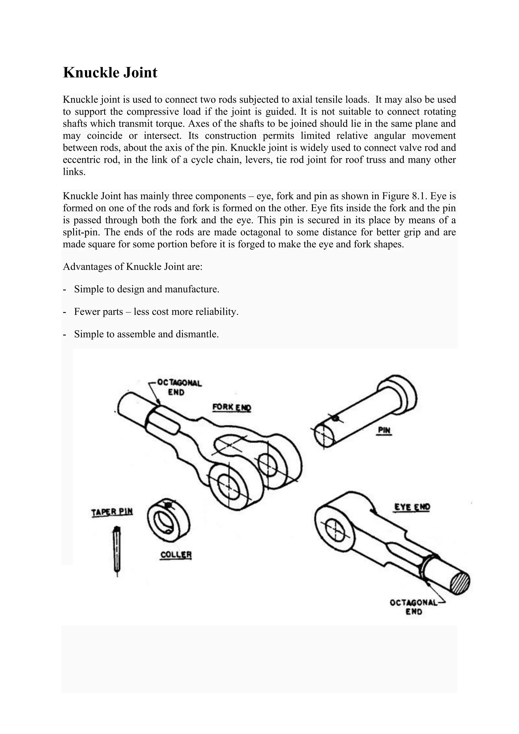
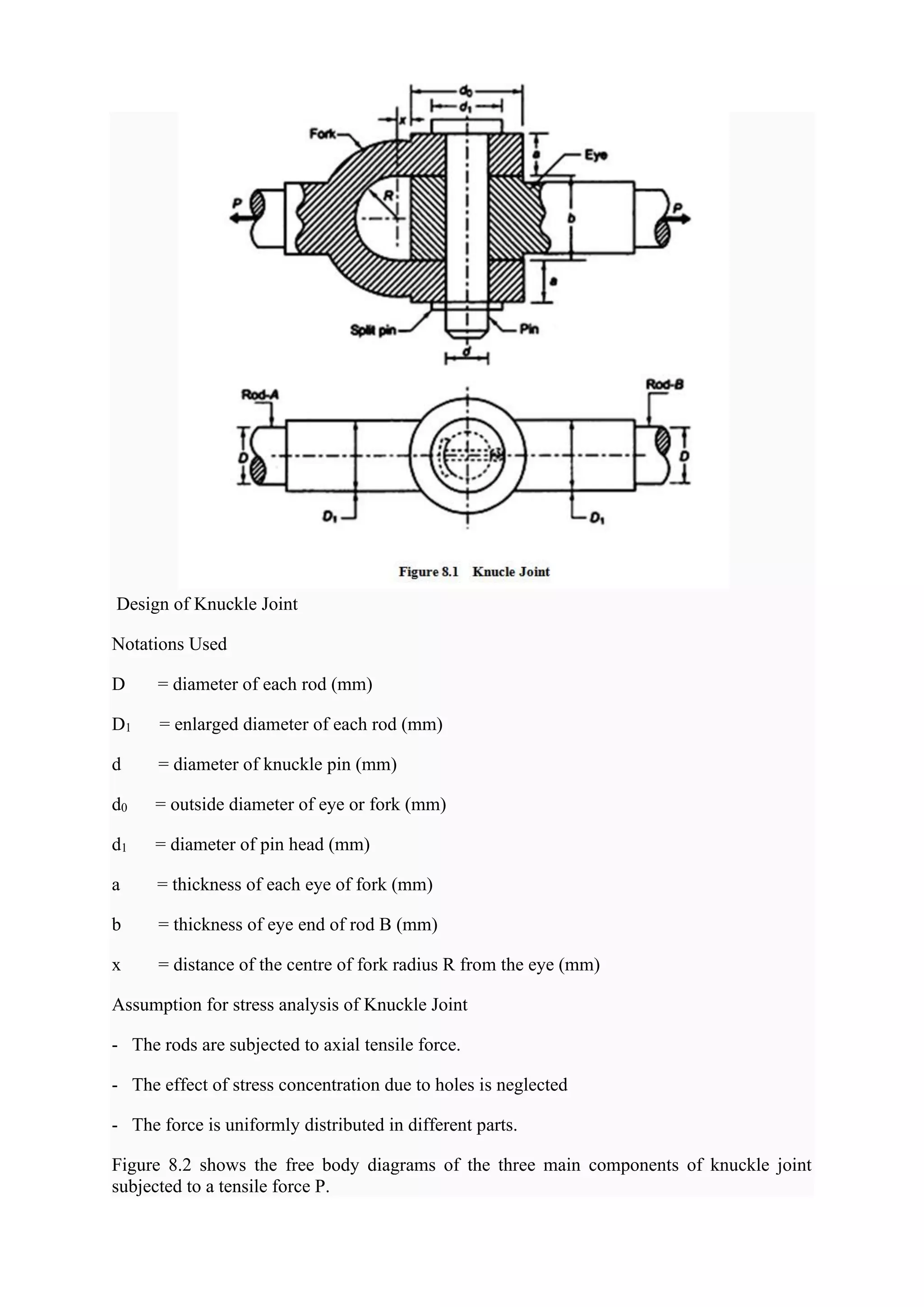
In order to find out various dimensions of the parts of a knuckle joint, failures in different
parts and at different x-sections are considered. The stresses developed in the components
should be less than the corresponding permissible values of stress. So, for each type of
failure, one strength equation is written and these strength equations are then used to find
various dimensions of the knuckle joint. Some empirical relations are also used to find the
dimensions.
Possible Failure Modes of Knuckle Joint
Tensile Failure of Rods
Each rod is subjected to a tensile force P.
where [σ] = allowable tensile stress for the material selected.
Shear Failure of Pin:
Total Area that resists the shear failure = 2*(
𝜫
𝟒
𝒅𝟐
)
where ɽ = allowable shear stress for the material selected.
Crushing Failure of Pin in Eye:
Projected Area of Pin in the eye = b d
where [σc] = allowable compressive stress for the material selected.
Crushing Failure of Pin in Fork:
Projected Area of Pin in the fork = 2 a d ,

Bending Failure of Pin:
When the pin is tight in the eye and fork, failure occurs due to shear, but when it is loose, it is
subjected to bending moment. It is assumed that: Load acting on the pin is uniformly
distributed in the eye and uniformly varying in the two parts of the fork.
Maximum Bending Moment (at centre) = M=
𝑃
2
(
𝑏
2
+
𝑎
3
) −
𝑃
2
×
𝑏
4
M=
𝑃
2
(
𝑏
4
+
𝑎
3
)
Maximum Bending Stress in the pin,
Where I=
𝜫
𝟔𝟒
𝒅𝟒
and y= d/2
Tensile Failure of Eye:
Area of the weakest section of eye resisting tensile failure = b (d0 – d)
Maximum Tensile Stress in eye,
Shear Failure of Eye:
The eye is subjected to double shear
Total area resisting shear =b(d0-d)
Maximum Shear Stress in eye =
Tensile Failure of Fork:
Area of the weakest section of fork resisting tensile failure = 2a (d0 – d)
Maximum Tensile Stress in fork =
Shear Failure of Fork:
Each of the two parts of the fork is subjected to double shear
Area of the weakest section of fork resisting shear failure = 2a (d0 – d)
Maximum Shear Stress in fork =

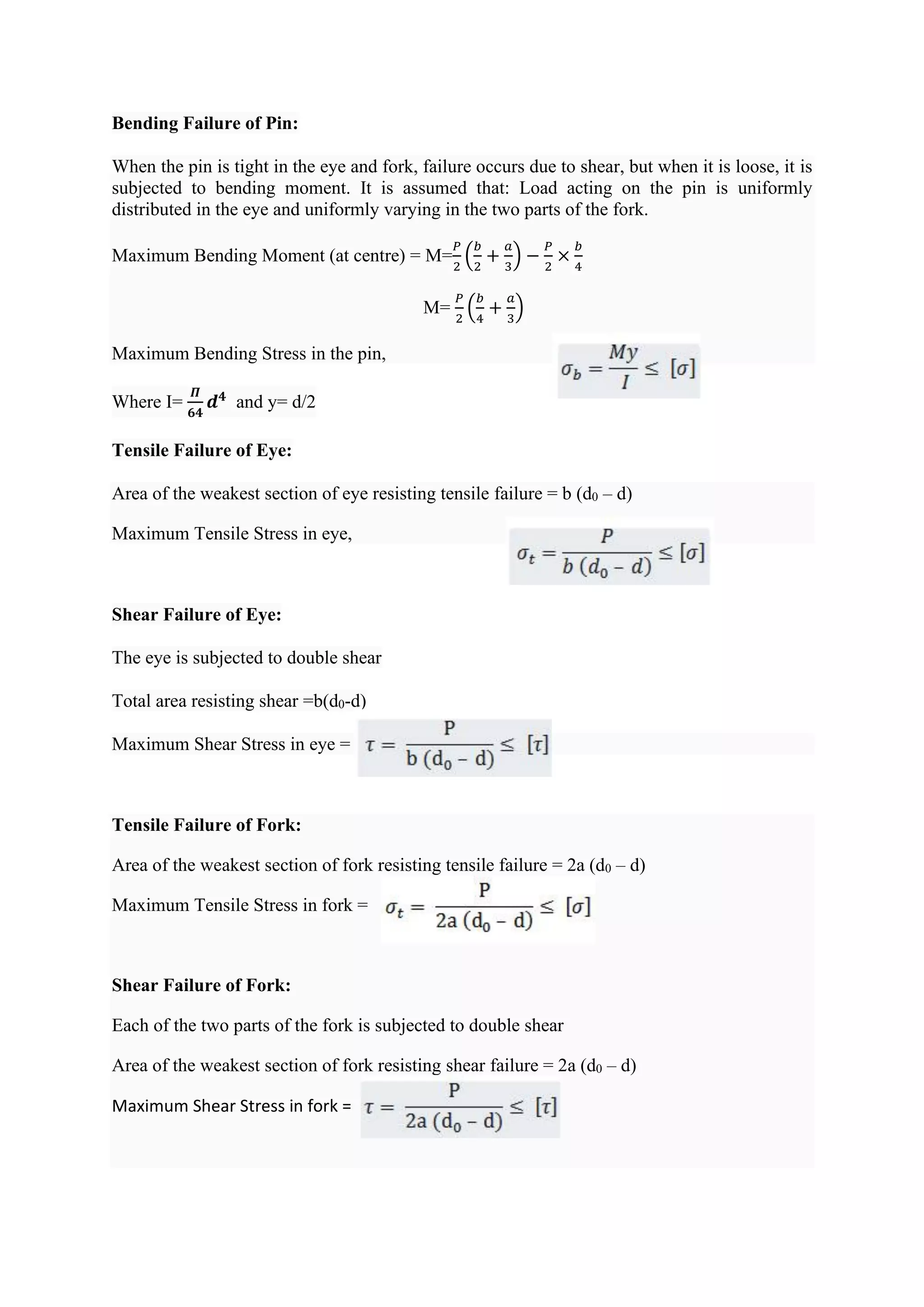
Design Procedure for Knuckle Joint
Some standard proportions for dimensions of the knuckle joint are taken as:
D1 = 1.1 D, d = D, d0 = 2d, a= 0.75 D, b = 1.25 D , d1 = 1.5 d & x = 10 mm
Dimensions can be determined using these empirical relations and the strength equations can
be then used as a check. By doing so the standard proportions of the joint can be maintained.
The other method, of designing it, can be making the use of above strength equations to find
the dimensions mathematically.
Procedure to determine various dimensions of knuckle joint is as follows:
i) Calculate the Diameter of each rod
ii) Calculate D1 for each rod using empirical relation [D1 = 1.1D]
iii) Calculate dimensions a and b also using empirical relations a = 0.75 D & b = 1.25 D
iv) Calculate diameter of the pin by shear and bending consideration and select the diameter
which is maximum.
And
Where M=
𝑃
2
(
𝑏
4
+
𝑎
3
), y= d/2 and I=
𝜫
𝟔𝟒
𝒅𝟒
v) Calculate dimensions d0 and d1 using empirical relations d0 = 2d and d1 = 1.5d
vi) Check the tensile, crushing and shear stresses in the eye
vii) Check the tensile, crushing and shear stresses in the fork

DESIGN OF COUPLINGS
Couplings are used to connect two rotating shafts to transmit torque from one to the other.
For example coupling is used to connect the output shaft of an electric motor to the input
shaft of a hydraulic pump.
Types of Shafts Couplings
Rigid Couplings
Rigid Couplings are used to connect two shafts which are perfectly aligned. These are simple
and inexpensive.
Rigid Couplings are of following types:
1. Sleeve or Muff Coupling
2. Clamp or Split-muff or Compression Coupling
3. Flange Coupling
Flexible Couplings
Flexible couplings are used to connect two shafts having lateral or angular misalignment.
Flexible elements provided in flexible coupling absorb shocks and vibrations.
Flexible Couplings are of following types:
1. Bushed pin type Coupling
2. Universal Coupling
3. Oldham Coupling
Flange Coupling
Flange coupling consists of two flanges keyed to the shafts. The flanges are connected
together by means of bolts arranged on a circle concentric to shaft. Power is transmitted from
driving shaft to flange on driving shaft through key, from flange on driving shaft to the flange
on driven shaft through bolts and then to the driven shaft through key again. Projection is
provided on one of the flanges and a corresponding recess is provided in the other for proper
alignment. Flange coupling is of two types – unprotected and protected. These are shown in
Figure 16.3. If in case failure of bolts occurs during the operation, the bolts may hit the
operator in case of unprotected flange coupling. To avoid this, protective circumferential
flanges are provided in the protected type flange coupling.
Flange of a protected type flange coupling has three distinct regions – inner hub, flanges and
protective circumferential flanges. Following standard proportions are used in the design of
flange coupling:
Outer diameter of hub, D = 2 d
Pitch circle diameter of bolts, D1 = 3 d
Outer diameter of flange, D2 = 4 d

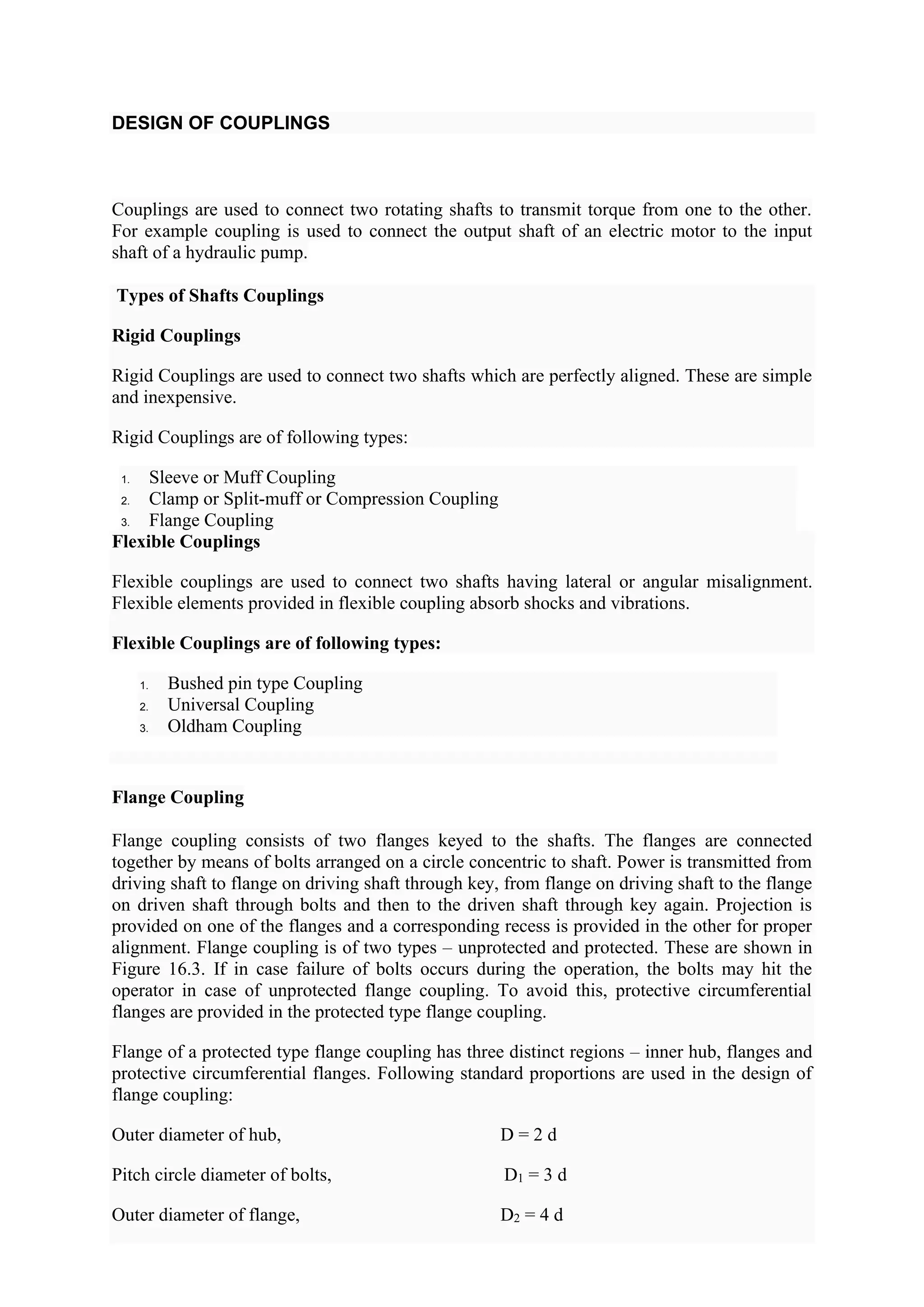
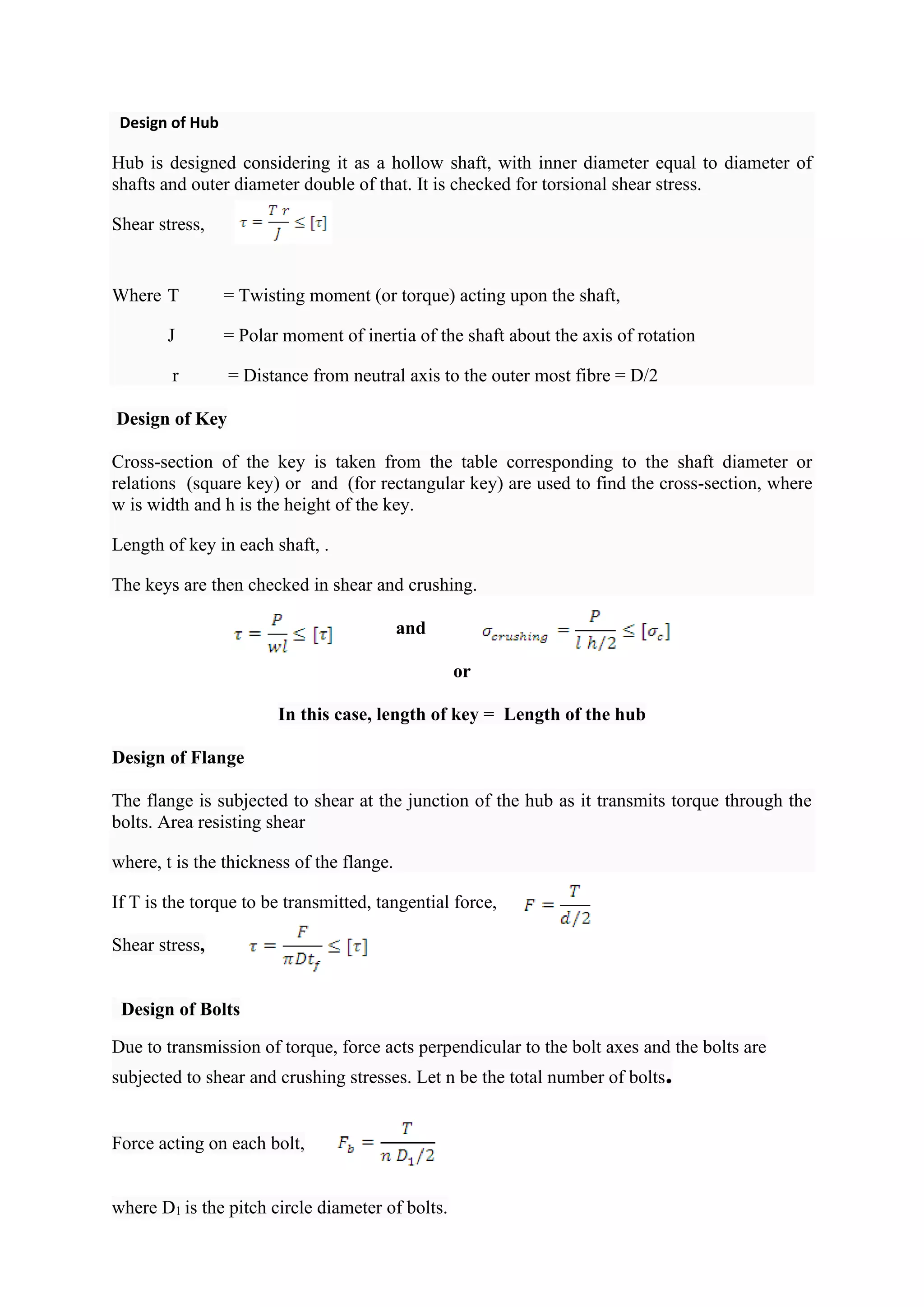
Length of the hub, L = 1.5 d
Thickness of flange, tf = 0.5 d
Thickness of protective circumferential flange, tp = 0.25 d
where d is the diameter of shafts to be coupled.
Design of flange coupling
Design of Shafts
Shafts are designed on the basis of torsional shear stress induced because of the torque to be
transmitted. Shear stress induced in shaft for transmitting torque, T is given by,
Where T = Twisting moment (or torque) acting upon the shaft,
J = Polar moment of inertia of the shaft about the axis of rotation
R = Distance from neutral axis to the outer most fibre = d/2
So dimensions of the shaft can be determined from above relation for a known value of
allowable shear stress, [τ].

Design of Hub
Hub is designed considering it as a hollow shaft, with inner diameter equal to diameter of
shafts and outer diameter double of that. It is checked for torsional shear stress.
Shear stress,
Where T = Twisting moment (or torque) acting upon the shaft,
J = Polar moment of inertia of the shaft about the axis of rotation
r = Distance from neutral axis to the outer most fibre = D/2
Design of Key
Cross-section of the key is taken from the table corresponding to the shaft diameter or
relations (square key) or and (for rectangular key) are used to find the cross-section, where
w is width and h is the height of the key.
Length of key in each shaft, .
The keys are then checked in shear and crushing.
and
or
In this case, length of key = Length of the hub
Design of Flange
The flange is subjected to shear at the junction of the hub as it transmits torque through the
bolts. Area resisting shear
where, t is the thickness of the flange.
If T is the torque to be transmitted, tangential force,
Shear stress,
Design of Bolts
Due to transmission of torque, force acts perpendicular to the bolt axes and the bolts are
subjected to shear and crushing stresses. Let n be the total number of bolts.
Force acting on each bolt,
where D1 is the pitch circle diameter of bolts.

Area resisting shear
where, dc = core diameter of bolts
Shear stress
Area under crushing
Crushing stress,
References:
1. Design of Machine Elements by VB Bhandari
2. Analysis and Design of Machine Elements by VK Jadon
3. A Text Book of Machine Design by RS Khurmi

Tom&amp;md notes module 03

More Related Content

What's hot

Similar to Tom&amp;md notes module 03

More from Ashish Mishra

Recently uploaded

Tom&amp;md notes module 03

Tom&md notes module 03

Similar to Tom&md notes module 03

Tom&md notes module 03